waveorder 2.2.0__py3-none-any.whl → 2.2.0rc0__py3-none-any.whl

waveorder/visuals/matplotlib_visuals.py

@@ -1,335 +0,0 @@
-import matplotlib.pyplot as plt
-import numpy as np
-
-
-def plot_5d_ortho(
-    rcCzyx_data: np.ndarray,
-    filename: str,
-    voxel_size: tuple[float, float, float],
-    zyx_slice: tuple[int, int, int],
-    color_funcs: list[list[callable]],
-    row_labels: list[str] = None,
-    column_labels: list[str] = None,
-    rose_path: str = None,
-    inches_per_column: float = 1.5,
-    label_size: int = 1,
-    ortho_line_width: float = 0.5,
-    row_column_line_width: float = 0.5,
-    xyz_labels: bool = True,
-    background_color: str = "white",
-    **kwargs: dict,
-) -> None:
-    """
-    Plot 5D multi-channel data in a grid or ortho-slice views.
-
-    Input data is a 6D array with (row, column, channels, Z, Y, X) dimensions.
-    
-    `color_funcs` permits different RGB color maps for each row and column.
-
-    Parameters
-    ----------
-    rcCzyx_data : numpy.ndarray
-        5D array with shape (R, C, Ch, Z, Y, X) containing the data to plot.
-        [r]ows and [c]olumns form a grid
-        [C]hannels contain multiple color channels
-        [ZYX] contain 3D volumes. 
-    filename : str
-        Path to save the output plot.
-    voxel_size : tuple[float, float, float]
-        Size of each voxel in (Z, Y, X) dimensions.
-    zyx_slice : tuple[int, int, int]
-        Indices of the ortho-slices to plot in (Z, Y, X) indices.
-    color_funcs : list[list[callable]]
-        A list of lists of callables, one for each element of the plot grid, 
-        with len(color_funcs) == R and len(colors_funcs[0] == C). 
-        Each callable accepts [C]hannel arguments and returns RGB color values,
-        enabling different RGB color maps for each member of the grid.
-    row_labels : list[str], optional
-        Labels for the rows, by default None.
-    column_labels : list[str], optional
-        Labels for the columns, by default None.
-    rose_path : str, optional
-        Path to an image to display in the top-left corner, by default None.
-    inches_per_column : float, optional
-        Width of each column in inches, by default 1.5.
-    label_size : int, optional
-        Size of the labels, by default 1.
-    ortho_line_width : float, optional
-        Width of the orthogonal lines, by default 0.5.
-    row_column_line_width : float, optional
-        Width of the lines between rows and columns, by default 0.5.
-    xyz_labels : bool, optional
-        Whether to display XYZ labels, by default True.
-    background_color : str, optional
-        Background color of the plot, by default "white".
-    **kwargs : dict
-        Additional keyword arguments passed to color_funcs.
-    """
-    R, C, Ch, Z, Y, X = rcCzyx_data.shape
-
-    # Extent
-    dZ, dY, dX = Z * voxel_size[0], Y * voxel_size[1], X * voxel_size[2]
-
-    assert R == len(row_labels)
-    assert C == len(column_labels)
-    assert zyx_slice[0] < Z and zyx_slice[1] < Y and zyx_slice[2] < X
-    assert zyx_slice[0] >= 0 and zyx_slice[1] >= 0 and zyx_slice[2] >= 0
-
-    assert R == len(color_funcs)
-    for color_func_row in color_funcs:
-        if isinstance(color_func_row, list):
-            assert len(color_func_row) == C
-        else:
-            color_func_row = [color_func_row] * C
-
-    n_rows = 1 + (2 * R)
-    n_cols = 1 + (2 * C)
-
-    width_ratios = [label_size] + C * [1, dZ / dX]
-    height_ratios = [label_size] + R * [dY / dX, dZ / dX]
-
-    fig_width = np.array(width_ratios).sum() * inches_per_column
-    fig_height = np.array(height_ratios).sum() * inches_per_column
-
-    fig, axes = plt.subplots(
-        n_rows,
-        n_cols,
-        figsize=(fig_width, fig_height),
-        gridspec_kw={
-            "wspace": 0.05,
-            "hspace": 0.05,
-            "width_ratios": width_ratios,
-            "height_ratios": height_ratios,
-        },
-    )
-    fig.patch.set_facecolor(background_color)
-    for ax in axes.flat:
-        ax.set_facecolor(background_color)
-
-    if rose_path is not None:
-        axes[0, 0].imshow(plt.imread(rose_path))
-
-    for i in range(n_rows):
-        for j in range(n_cols):
-            # Add labels
-            if (i == 0 and (j - 1) % 2 == 0) or (j == 0 and (i - 1) % 2 == 0):
-                axes[i, j].text(
-                    0.5,
-                    0.5,
-                    index,
-                    horizontalalignment="center",
-                    verticalalignment="center",
-                    fontsize=10 * label_size,
-                    color="black",
-                )
-
-            # Add data
-            if i > 0 and j > 0:
-                color_func = color_funcs[int((i - 1) / 2)][int((j - 1) / 2)]
-
-                Cyx_data = rcCzyx_data[
-                    int((i - 1) / 2), int((j - 1) / 2), :, zyx_slice[0]
-                ]
-                Cyz_data = rcCzyx_data[
-                    int((i - 1) / 2), int((j - 1) / 2), :, :, :, zyx_slice[2]
-                ].transpose(0, 2, 1)
-                Czx_data = rcCzyx_data[
-                    int((i - 1) / 2), int((j - 1) / 2), :, :, zyx_slice[1]
-                ]
-
-                # YX
-                if (i - 1) % 2 == 0 and (j - 1) % 2 == 0:
-                    axes[i, j].imshow(
-                        color_func(*Cyx_data, **kwargs),
-                        aspect=voxel_size[1] / voxel_size[2],
-                    )
-                # YZ
-                elif (i - 1) % 2 == 0 and (j - 1) % 2 == 1:
-                    axes[i, j].imshow(
-                        color_func(*Cyz_data, **kwargs),
-                        aspect=voxel_size[1] / voxel_size[0],
-                    )
-                # XZ
-                elif (i - 1) % 2 == 1 and (j - 1) % 2 == 0:
-                    axes[i, j].imshow(
-                        color_func(*Czx_data, **kwargs),
-                        aspect=voxel_size[0] / voxel_size[2],
-                    )
-
-            # Draw lines between rows and cols
-            top = axes[0, 0].get_position().y1
-            bottom = axes[-1, -1].get_position().y0
-            left = axes[0, 0].get_position().x0
-            right = axes[-1, -1].get_position().x1
-            if i == 0 and (j - 1) % 2 == 0:
-                left_edge = (
-                    axes[0, j].get_position().x0
-                    + axes[0, j - 1].get_position().x1
-                ) / 2
-                fig.add_artist(
-                    plt.Line2D(
-                        [left_edge, left_edge],
-                        [bottom, top],
-                        transform=fig.transFigure,
-                        color="black",
-                        lw=row_column_line_width,
-                    )
-                )
-            if j == 0 and (i - 1) % 2 == 0:
-                top_edge = (
-                    axes[i, 0].get_position().y1
-                    + axes[i - 1, 0].get_position().y0
-                ) / 2
-                fig.add_artist(
-                    plt.Line2D(
-                        [left, right],
-                        [top_edge, top_edge],
-                        transform=fig.transFigure,
-                        color="black",
-                        lw=row_column_line_width,
-                    )
-                )
-
-            # Remove ticks and spines
-            axes[i, j].tick_params(
-                left=False, bottom=False, labelleft=False, labelbottom=False
-            )
-            axes[i, j].spines["top"].set_visible(False)
-            axes[i, j].spines["right"].set_visible(False)
-            axes[i, j].spines["bottom"].set_visible(False)
-            axes[i, j].spines["left"].set_visible(False)
-
-    yx_slice_color = "green"
-    yz_slice_color = "red"
-    zx_slice_color = "blue"
-
-    # Label orthogonal slices
-    add_ortho_lines_to_axis(
-        axes[1, 1],
-        (zyx_slice[1], zyx_slice[2]),
-        ("y", "x") if xyz_labels else ("", ""),
-        yx_slice_color,
-        yz_slice_color,
-        zx_slice_color,
-        ortho_line_width,
-    )  # YX axis
-
-    add_ortho_lines_to_axis(
-        axes[2, 1],
-        (zyx_slice[0], zyx_slice[2]),
-        ("z", "x") if xyz_labels else ("", ""),
-        zx_slice_color,
-        yz_slice_color,
-        yx_slice_color,
-        ortho_line_width,
-    )  # ZX axis
-
-    add_ortho_lines_to_axis(
-        axes[1, 2],
-        (zyx_slice[1], zyx_slice[0]),
-        ("y", "z") if xyz_labels else ("", ""),
-        yz_slice_color,
-        yx_slice_color,
-        zx_slice_color,
-        ortho_line_width,
-    )  # YZ axis
-
-    print(f"Saving {filename}")
-    fig.savefig(filename, dpi=400, format="pdf", bbox_inches="tight")
-
-
-def add_ortho_lines_to_axis(
-    axis: plt.Axes,
-    yx_slice: tuple[int, int],
-    axis_labels: tuple[str, str],
-    outer_color: str,
-    vertical_color: str,
-    horizontal_color: str,
-    line_width: float = 0,
-    text_color: str = "white",
-) -> None:
-    """
-    Add orthogonal lines and labels to a given axis.
-
-    Parameters
-    ----------
-    axis : matplotlib.axes.Axes
-        The axis to which the orthogonal lines and labels will be added.
-    yx_slice : tuple[int, int]
-        The (Y, X) slice indices for the orthogonal lines.
-    axis_labels : tuple[str, str]
-        The labels for the Y and X axes.
-    outer_color : str
-        The color of the outer rectangle.
-    vertical_color : str
-        The color of the vertical line.
-    horizontal_color : str
-        The color of the horizontal line.
-    line_width : float, optional
-        The width of the lines, by default 0.
-    text_color : str, optional
-        The color of the text labels, by default "white".
-    """
-    xmin, xmax = axis.get_xlim()
-    ymin, ymax = axis.get_ylim()
-
-    # Axis labels
-    horizontal_axis_label_pos = (0.1, 0.975)
-    vertical_axis_label_pos = (0.025, 0.9)
-    axis.text(
-        horizontal_axis_label_pos[0],
-        horizontal_axis_label_pos[1],
-        axis_labels[1],
-        horizontalalignment="left",
-        verticalalignment="top",
-        transform=axis.transAxes,
-        fontsize=5,
-        color=text_color,
-    )
-
-    axis.text(
-        vertical_axis_label_pos[0],
-        vertical_axis_label_pos[1],
-        axis_labels[0],
-        horizontalalignment="left",
-        verticalalignment="top",
-        transform=axis.transAxes,
-        fontsize=5,
-        color=text_color,
-    )
-
-    # Outer rectangle
-    axis.add_artist(
-        plt.Rectangle(
-            (xmin, ymin),
-            xmax - xmin,
-            ymax - ymin,
-            linewidth=line_width,
-            edgecolor=outer_color,
-            facecolor="none",
-            transform=axis.transData,
-            clip_on=False,
-        )
-    )
-
-    # Horizontal line
-    axis.add_artist(
-        plt.Line2D(
-            [xmin, xmax],
-            [yx_slice[0], yx_slice[0]],
-            transform=axis.transData,
-            color=horizontal_color,
-            lw=line_width,
-        )
-    )
-
-    # Vertical line
-    axis.add_artist(
-        plt.Line2D(
-            [yx_slice[1], yx_slice[1]],
-            [ymin, ymax],
-            transform=axis.transData,
-            color=vertical_color,
-            lw=line_width,
-        )
-    )

waveorder/visuals/napari_visuals.py

@@ -1,77 +0,0 @@
-from waveorder.visuals.utils import complex_tensor_to_rgb
-from typing import TYPE_CHECKING
-
-import numpy as np
-import torch
-
-
-def add_transfer_function_to_viewer(
-    viewer: "napari.Viewer",
-    transfer_function: torch.Tensor,
-    zyx_scale: tuple[float, float, float],
-    layer_name: str = "Transfer Function",
-    clim_factor: float = 1.0,
-    complex_rgb: bool = False,
-):
-    zyx_shape = transfer_function.shape[-3:]
-    lim = torch.max(torch.abs(transfer_function)) * clim_factor
-    voxel_scale = np.array(
-        [
-            zyx_shape[0] * zyx_scale[0],
-            zyx_shape[1] * zyx_scale[1],
-            zyx_shape[2] * zyx_scale[2],
-        ]
-    )
-    shift_dims = (-3, -2, -1)
-
-    if complex_rgb:
-        rgb_transfer_function = complex_tensor_to_rgb(
-            np.array(torch.fft.ifftshift(transfer_function, dim=shift_dims)),
-            saturate_clim_fraction=clim_factor,
-        )
-        viewer.add_image(
-            rgb_transfer_function,
-            scale=1 / voxel_scale,
-            name=layer_name,
-        )
-    else:
-        viewer.add_image(
-            torch.fft.ifftshift(torch.real(transfer_function), dim=shift_dims)
-            .cpu()
-            .numpy(),
-            colormap="bwr",
-            contrast_limits=(-lim, lim),
-            scale=1 / voxel_scale,
-            name="Re(" + layer_name + ")",
-        )
-        if transfer_function.dtype == torch.complex64:
-            viewer.add_image(
-                torch.fft.ifftshift(
-                    torch.imag(transfer_function), dim=shift_dims
-                )
-                .cpu()
-                .numpy(),
-                colormap="bwr",
-                contrast_limits=(-lim, lim),
-                scale=1 / voxel_scale,
-                name="Im(" + layer_name + ")",
-            )
-
-    viewer.dims.current_step = (0,) * (transfer_function.ndim - 3) + (
-        zyx_shape[0] // 2,
-        zyx_shape[1] // 2,
-        zyx_shape[2] // 2,
-    )
-
-    # Show XZ view by default, and only allow rolling between XY and XZ
-    viewer.dims.order = list(range(transfer_function.ndim - 3)) + [
-        transfer_function.ndim - 2,
-        transfer_function.ndim - 3,
-        transfer_function.ndim - 1,
-    ]
-    viewer.dims.rollable = (False,) * (transfer_function.ndim - 3) + (
-        True,
-        True,
-        False,
-    )
-    viewer.dims.axis_labels = ("DATA", "OBJECT", "Z", "Y", "X")

waveorder/visuals/utils.py

@@ -1,31 +0,0 @@
-import numpy as np
-import matplotlib.colors as mcolors
-
-
-# Main function to convert a complex-valued torch tensor to RGB numpy array
-# with red at +1, green at +i, blue at -1, and purple at -i
-def complex_tensor_to_rgb(array, saturate_clim_fraction=1.0):
-
-    # Calculate magnitude and phase for the entire array
-    magnitude = np.abs(array)
-    phase = np.angle(array)
-
-    # Normalize phase to [0, 1]
-    hue = (phase + np.pi) / (2 * np.pi)
-    hue = np.mod(hue + 0.5, 1)
-
-    # Normalize magnitude to [0, 1] for saturation
-    if saturate_clim_fraction is not None:
-        max_abs_val = np.amax(magnitude) * saturate_clim_fraction
-    else:
-        max_abs_val = 1.0
-
-    sat = magnitude / max_abs_val if max_abs_val != 0 else magnitude
-
-    # Create HSV array: hue, saturation, value (value is set to 1)
-    hsv = np.stack((hue, sat, np.ones_like(sat)), axis=-1)
-
-    # Convert the entire HSV array to RGB using vectorized conversion
-    rgb_array = mcolors.hsv_to_rgb(hsv)
-
-    return rgb_array

waveorder-2.2.0.dist-info/METADATA

@@ -1,186 +0,0 @@
-Metadata-Version: 2.1
-Name: waveorder
-Version: 2.2.0
-Summary: Wave-optical simulations and deconvolution of optical properties
-Author-email: CZ Biohub SF <compmicro@czbiohub.org>
-Maintainer-email: Talon Chandler <talon.chandler@czbiohub.org>, Shalin Mehta <shalin.mehta@czbiohub.org>
-License: BSD 3-Clause License
-        
-        Copyright (c) 2019, Chan Zuckerberg Biohub
-        
-        Redistribution and use in source and binary forms, with or without
-        modification, are permitted provided that the following conditions are met:
-        
-        1. Redistributions of source code must retain the above copyright notice, this
-           list of conditions and the following disclaimer.
-        
-        2. Redistributions in binary form must reproduce the above copyright notice,
-           this list of conditions and the following disclaimer in the documentation
-           and/or other materials provided with the distribution.
-        
-        3. Neither the name of the copyright holder nor the names of its
-           contributors may be used to endorse or promote products derived from
-           this software without specific prior written permission.
-        
-        THIS SOFTWARE IS PROVIDED BY THE COPYRIGHT HOLDERS AND CONTRIBUTORS "AS IS"
-        AND ANY EXPRESS OR IMPLIED WARRANTIES, INCLUDING, BUT NOT LIMITED TO, THE
-        IMPLIED WARRANTIES OF MERCHANTABILITY AND FITNESS FOR A PARTICULAR PURPOSE ARE
-        DISCLAIMED. IN NO EVENT SHALL THE COPYRIGHT HOLDER OR CONTRIBUTORS BE LIABLE
-        FOR ANY DIRECT, INDIRECT, INCIDENTAL, SPECIAL, EXEMPLARY, OR CONSEQUENTIAL
-        DAMAGES (INCLUDING, BUT NOT LIMITED TO, PROCUREMENT OF SUBSTITUTE GOODS OR
-        SERVICES; LOSS OF USE, DATA, OR PROFITS; OR BUSINESS INTERRUPTION) HOWEVER
-        CAUSED AND ON ANY THEORY OF LIABILITY, WHETHER IN CONTRACT, STRICT LIABILITY,
-        OR TORT (INCLUDING NEGLIGENCE OR OTHERWISE) ARISING IN ANY WAY OUT OF THE USE
-        OF THIS SOFTWARE, EVEN IF ADVISED OF THE POSSIBILITY OF SUCH DAMAGE.
-        
-Project-URL: Homepage, https://github.com/mehta-lab/waveorder
-Project-URL: Repository, https://github.com/mehta-lab/waveorder
-Project-URL: Issues, https://github.com/mehta-lab/waveorder/issues
-Keywords: simulation,optics,phase,scattering,polarization,label-free,permittivity,reconstruction-algorithm,qlipp,mipolscope,permittivity-tensor-imaging
-Classifier: Development Status :: 4 - Beta
-Classifier: Intended Audience :: Science/Research
-Classifier: License :: OSI Approved :: BSD License
-Classifier: Programming Language :: Python :: 3
-Classifier: Programming Language :: Python :: 3.10
-Classifier: Programming Language :: Python :: 3.11
-Classifier: Programming Language :: Python :: 3.12
-Classifier: Topic :: Scientific/Engineering
-Classifier: Topic :: Scientific/Engineering :: Image Processing
-Classifier: Topic :: Scientific/Engineering :: Bio-Informatics
-Classifier: Operating System :: POSIX :: Linux
-Classifier: Operating System :: Microsoft :: Windows
-Classifier: Operating System :: MacOS
-Requires-Python: >=3.10
-Description-Content-Type: text/markdown
-License-File: LICENSE
-Requires-Dist: numpy>=1.24
-Requires-Dist: matplotlib>=3.1.1
-Requires-Dist: scipy>=1.3.0
-Requires-Dist: pywavelets>=1.1.1
-Requires-Dist: ipywidgets>=7.5.1
-Requires-Dist: torch>=2.4.1
-Provides-Extra: dev
-Requires-Dist: pytest; extra == "dev"
-Requires-Dist: pytest-cov; extra == "dev"
-Provides-Extra: examples
-Requires-Dist: napari[all]; extra == "examples"
-Requires-Dist: jupyter; extra == "examples"
-
-# waveorder
-
-[![Python package index](https://img.shields.io/pypi/v/waveorder.svg)](https://pypi.org/project/waveorder)
-[![PyPI monthly downloads](https://img.shields.io/pypi/dm/waveorder.svg)](https://pypistats.org/packages/waveorder)
-[![Total downloads](https://pepy.tech/badge/waveorder)](https://pepy.tech/project/waveorder)
-[![GitHub contributors](https://img.shields.io/github/contributors-anon/mehta-lab/waveorder)](https://github.com/mehta-lab/waveorder/graphs/contributors)
-![GitHub Repo stars](https://img.shields.io/github/stars/mehta-lab/waveorder)
-![GitHub forks](https://img.shields.io/github/forks/mehta-lab/waveorder)
-![PyPI - Python Version](https://img.shields.io/pypi/pyversions/waveorder)
-
-
-This computational imaging library enables wave-optical simulation and reconstruction of optical properties that report microscopic architectural order.
-
-## Computational label-agnostic imaging
-
-https://github.com/user-attachments/assets/4f9969e5-94ce-4e08-9f30-68314a905db6
-
-`waveorder` enables simulations and reconstructions of label-agnostic microscopy data as described in the following [preprint](https://arxiv.org/abs/2412.09775)
-<details>	
-<summary> Chandler et al. 2024 </summary>
-<pre><code>
-@article{chandler_2024,
-    author = {Chandler, Talon and Hirata-Miyasaki, Eduardo and Ivanov, Ivan E. and Liu, Ziwen and Sundarraman, Deepika and Ryan, Allyson Quinn and Jacobo, Adrian and Balla, Keir and Mehta, Shalin B.},
-	title = {waveOrder: generalist framework for label-agnostic computational microscopy},
-	journal = {arXiv},
-	year = {2024},
-	month = dec,
-	eprint = {2412.09775},
-	doi = {10.48550/arXiv.2412.09775}
-}
-</code></pre>
-</details>
-
-Specifically, `waveorder` enables simulation and reconstruction of 2D or 3D:
-
-1. __phase, projected retardance, and in-plane orientation__ from a polarization-diverse volumetric brightfield acquisition ([QLIPP](https://elifesciences.org/articles/55502)),
-
-2. __phase__ from a volumetric brightfield acquisition ([2D phase](https://www.osapublishing.org/ao/abstract.cfm?uri=ao-54-28-8566)/[3D phase](https://www.osapublishing.org/ao/abstract.cfm?uri=ao-57-1-a205)),
-
-3. __phase__ from an illumination-diverse volumetric acquisition ([2D](https://www.osapublishing.org/oe/fulltext.cfm?uri=oe-23-9-11394&id=315599)/[3D](https://www.osapublishing.org/boe/fulltext.cfm?uri=boe-7-10-3940&id=349951) differential phase contrast),
-
-4. __fluorescence density__ from a widefield volumetric fluorescence acquisition (fluorescence deconvolution).  
-
-The [examples](https://github.com/mehta-lab/waveorder/tree/main/examples) demonstrate simulations and reconstruction for 2D QLIPP, 3D PODT, 3D fluorescence deconvolution, and 2D/3D PTI methods.
-
-If you are interested in deploying QLIPP, phase from brightfield, or fluorescence deconvolution for label-agnostic imaging at scale, checkout our [napari plugin](https://www.napari-hub.org/plugins/recOrder-napari),  [`recOrder-napari`](https://github.com/mehta-lab/recOrder).
-
-## Permittivity tensor imaging 
-
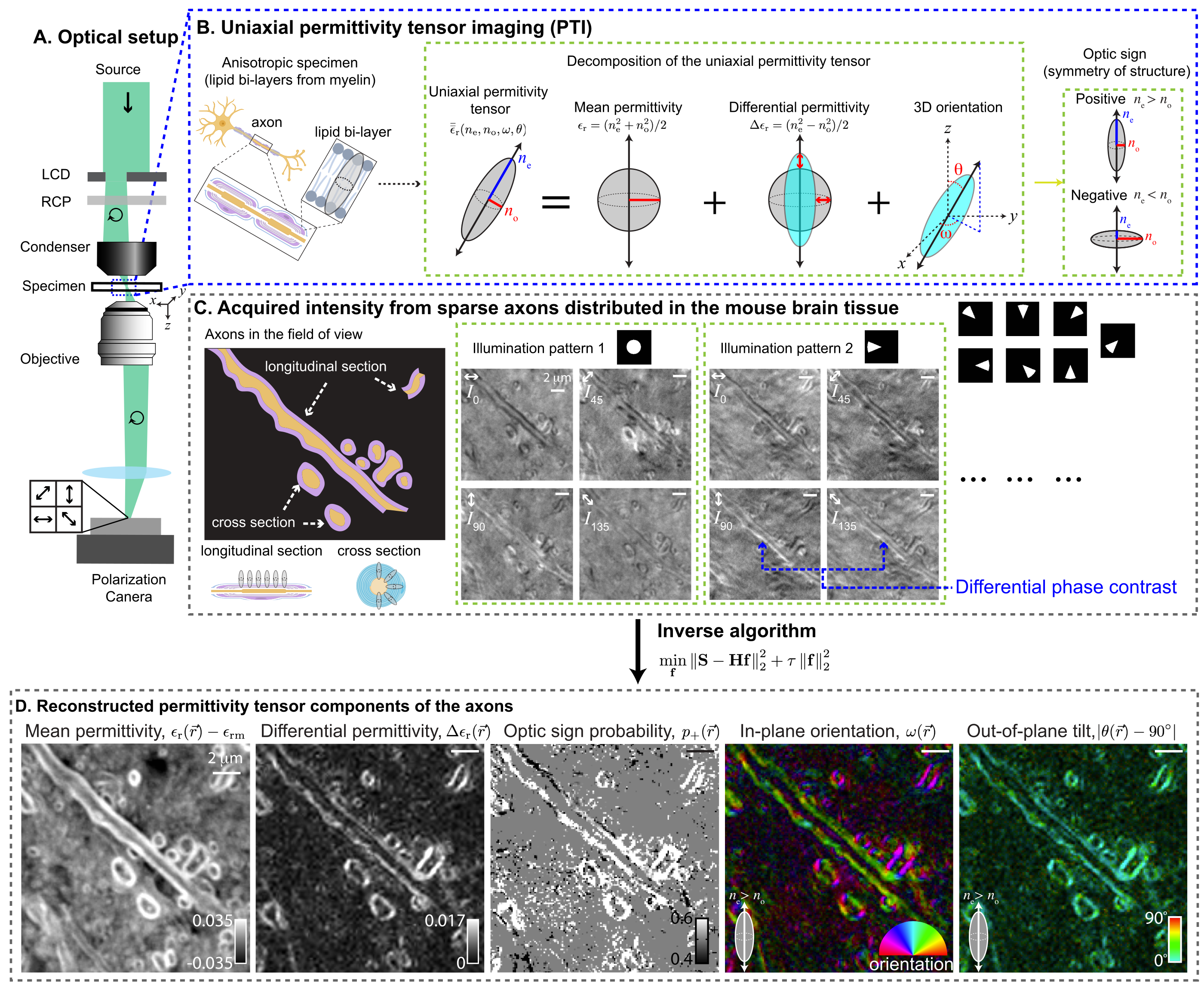
-Additionally, `waveorder` enabled the development of a new label-free imaging method, __permittivity tensor imaging (PTI)__, that measures density and  3D orientation of biomolecules with diffraction-limited resolution. These measurements are reconstructed from polarization-resolved images acquired with a sequence of oblique illuminations.
-
-The acquisition, calibration, background correction, reconstruction, and applications of PTI are described in the following [paper](https://doi.org/10.1101/2020.12.15.422951) published in Nature Methods:
-
-<details>
-<summary> Yeh et al. 2024 </summary>
-<pre><code>
-@article{yeh_2024,
-	author = {Yeh, Li-Hao and Ivanov, Ivan E. and Chandler, Talon and Byrum, Janie R. and Chhun, Bryant B. and Guo, Syuan-Ming and Foltz, Cameron and Hashemi, Ezzat and Perez-Bermejo, Juan A. and Wang, Huijun and Yu, Yanhao and Kazansky, Peter G. and Conklin, Bruce R. and Han, May H. and Mehta, Shalin B.},
-	title = {Permittivity tensor imaging: modular label-free imaging of 3D dry mass and 3D orientation at high resolution},
-	journal = {Nature Methods},
-	volume = {21},
-	number = {7},
-	pages = {1257--1274},
-	year = {2024},
-	month = jul,
-	issn = {1548-7105},
-	publisher = {Nature Publishing Group},
-	doi = {10.1038/s41592-024-02291-w}
-}
-</code></pre>
-</details>
-
-PTI provides volumetric reconstructions of mean permittivity ($\propto$ material density), differential permittivity ($\propto$ material anisotropy), 3D orientation, and optic sign. The following figure summarizes PTI acquisition and reconstruction with a small optical section of the mouse brain tissue:
-
-![Data_flow](https://github.com/mehta-lab/waveorder/blob/main/readme.png?raw=true)
-
-## Examples
-The [examples](https://github.com/mehta-lab/waveorder/tree/main/examples) illustrate simulations and reconstruction for 2D QLIPP, 3D phase from brightfield, and 2D/3D PTI methods.
-
-If you are interested in deploying QLIPP or phase from brightbrield, or fluorescence deconvolution for label-agnostic imaging at scale, checkout our [napari plugin](https://www.napari-hub.org/plugins/recOrder-napari),  [`recOrder-napari`](https://github.com/mehta-lab/recOrder).
-
-## Citation
-
-Please cite this repository, along with the relevant preprint or paper, if you use or adapt this code. The citation information can be found by clicking "Cite this repository" button in the About section in the right sidebar.
-
-## Installation
-
-Create a virtual environment:
-
-```sh
-conda create -y -n waveorder python=3.10
-conda activate waveorder
-```
-
-Install `waveorder` from PyPI:
-
-```sh
-pip install waveorder
-```
-
-Use `waveorder` in your scripts:
-
-```sh
-python
->>> import waveorder
-```
-
-(Optional) Install example dependencies, clone the repository, and run an example script:
-```sh
-pip install waveorder[examples]
-git clone https://github.com/mehta-lab/waveorder.git
-python waveorder/examples/models/phase_thick_3d.py
-```
-
-(M1 users) `pytorch` has [incomplete GPU support](https://github.com/pytorch/pytorch/issues/77764),
-so please use `export PYTORCH_ENABLE_MPS_FALLBACK=1`
-to allow some operators to fallback to CPU
-if you plan to use GPU acceleration for polarization reconstruction. 

waveorder-2.2.0.dist-info/RECORD

@@ -1,25 +0,0 @@
-waveorder/__init__.py,sha256=47DEQpj8HBSa-_TImW-5JCeuQeRkm5NMpJWZG3hSuFU,0
-waveorder/_version.py,sha256=pbL_Q6fDSZl5UbKP04ZFdzrJpd1PO1gH7IwJCwLV7mk,411
-waveorder/background_estimator.py,sha256=gCIO6-232H0CGH4o6gnqW9KSYGOrXf5E9nD67WeF304,12399
-waveorder/correction.py,sha256=N0Ic6mqw3U7mqow4dKTOkNx2QYOLwedGNH7HiKV-M6s,3460
-waveorder/focus.py,sha256=4mg84Fe4V-oFplsuaU_VQU1_TEDoEfPggIAv6Is2dE4,6312
-waveorder/optics.py,sha256=Z0N9IN5AJ563eOISlFVJLS5K7lyfSjOcHVkzcLSKP1E,44325
-waveorder/sampling.py,sha256=OAqlfjEemX6tQV2a2S8X0wQx9JCSykcvVxvKr1CY3H0,2521
-waveorder/stokes.py,sha256=Wk9ZimzICIZLh1CkB0kQSCSBLeugkDeydwXTPd-M-po,15186
-waveorder/util.py,sha256=goT2OD6Zej4v3RT1tu_XAQtDWi94HiDlL4pJk2itt6s,71272
-waveorder/waveorder_reconstructor.py,sha256=SSSru4TOLB1VUOWMLHzMSboMbazgfslFXrjOpnwmqFk,152107
-waveorder/waveorder_simulator.py,sha256=_HCmDZkACUGzgwnaI-q0PjsL1gRE55IQuaWw-wtAjCU,45856
-waveorder/models/inplane_oriented_thick_pol3d.py,sha256=jEpMcAZ6tIg9Kg-lHpbH0vBAphSGZGUAqLyDc0hv_bs,5979
-waveorder/models/inplane_oriented_thick_pol3d_vector.py,sha256=09-Qu6Ka3S2GmkcmGIyVbQCYP1I_S9O1HvDBZDQ7AlQ,10817
-waveorder/models/isotropic_fluorescent_thick_3d.py,sha256=TuE5QlScy6pdCZyrWJifJ6UJMQT15lv8HhkNa_cQfFs,6713
-waveorder/models/isotropic_thin_3d.py,sha256=c-1eKknNWKxDiMNUi0wBf6YeXhUQiUR-zguH8M7En_k,10941
-waveorder/models/phase_thick_3d.py,sha256=2gq5pd6BPxDmkqnf9bvbOfraD2CeGBr0GU1s9cYBTms,8374
-waveorder/visuals/jupyter_visuals.py,sha256=w-vlMtfyl3I1ACNfYIW4fbS9TIMAVittNj3GbjlRYz4,58121
-waveorder/visuals/matplotlib_visuals.py,sha256=e-4LrHPFU--j3gbUoZrO8WHpDIYNZDFu8vqBZyhyiG4,10922
-waveorder/visuals/napari_visuals.py,sha256=gI420pgOzun4Elx__txdk1eEBcTIBB6Gpln-6n8Wo1k,2385
-waveorder/visuals/utils.py,sha256=6vdZmpvFGHwSwxeV8vCKWQ0MBOrDokSIJhjdBtJLHeM,1002
-waveorder-2.2.0.dist-info/LICENSE,sha256=auz4oGH1A-xZtoiR2zuXIk-Hii4v9aGgFVBqn7nfpms,1509
-waveorder-2.2.0.dist-info/METADATA,sha256=D7tFPrufseWBEz4-kPpR6pejV_GtA91ll7SsO4u3qas,9677
-waveorder-2.2.0.dist-info/WHEEL,sha256=PZUExdf71Ui_so67QXpySuHtCi3-J3wvF4ORK6k_S8U,91
-waveorder-2.2.0.dist-info/top_level.txt,sha256=i3zReXiiMTnyPk93W7aEz_oEfsLnfR_Kzl7PW7kUslA,10
-waveorder-2.2.0.dist-info/RECORD,,