swesphere 0.3.0__py3-none-any.whl
This diff represents the content of publicly available package versions that have been released to one of the supported registries. The information contained in this diff is provided for informational purposes only and reflects changes between package versions as they appear in their respective public registries.
- swesphere/__init__.py +13 -0
- swesphere/climatology.py +38 -0
- swesphere/diagnostics.py +39 -0
- swesphere/dynamics.py +88 -0
- swesphere/forcing.py +26 -0
- swesphere/grid.py +161 -0
- swesphere/initial_conditions.py +160 -0
- swesphere/integrators.py +22 -0
- swesphere/model.py +89 -0
- swesphere/presets.py +64 -0
- swesphere-0.3.0.dist-info/METADATA +194 -0
- swesphere-0.3.0.dist-info/RECORD +15 -0
- swesphere-0.3.0.dist-info/WHEEL +5 -0
- swesphere-0.3.0.dist-info/licenses/LICENSE +21 -0
- swesphere-0.3.0.dist-info/top_level.txt +1 -0
swesphere/__init__.py
ADDED
|
@@ -0,0 +1,13 @@
|
|
|
1
|
+
"""swesphere: shallow-water equations on the sphere for data-assimilation testbeds.
|
|
2
|
+
|
|
3
|
+
from swesphere import presets, climatology
|
|
4
|
+
model, x0 = presets.two_jets()
|
|
5
|
+
S = climatology.build_climatology(model, x0, spinup_days=40, n_snapshots=200, every_days=2)
|
|
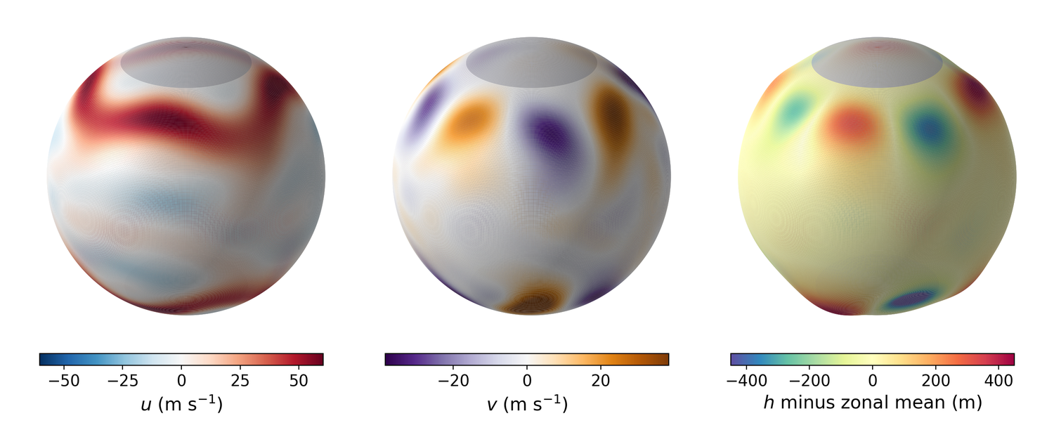
6
|
+
"""
|
|
7
|
+
from .model import SWEModel
|
|
8
|
+
from .grid import SphereGrid
|
|
9
|
+
from .forcing import ZonalRelaxation
|
|
10
|
+
from . import presets, climatology, initial_conditions, integrators, dynamics, diagnostics
|
|
11
|
+
|
|
12
|
+
__version__ = "0.3.0"
|
|
13
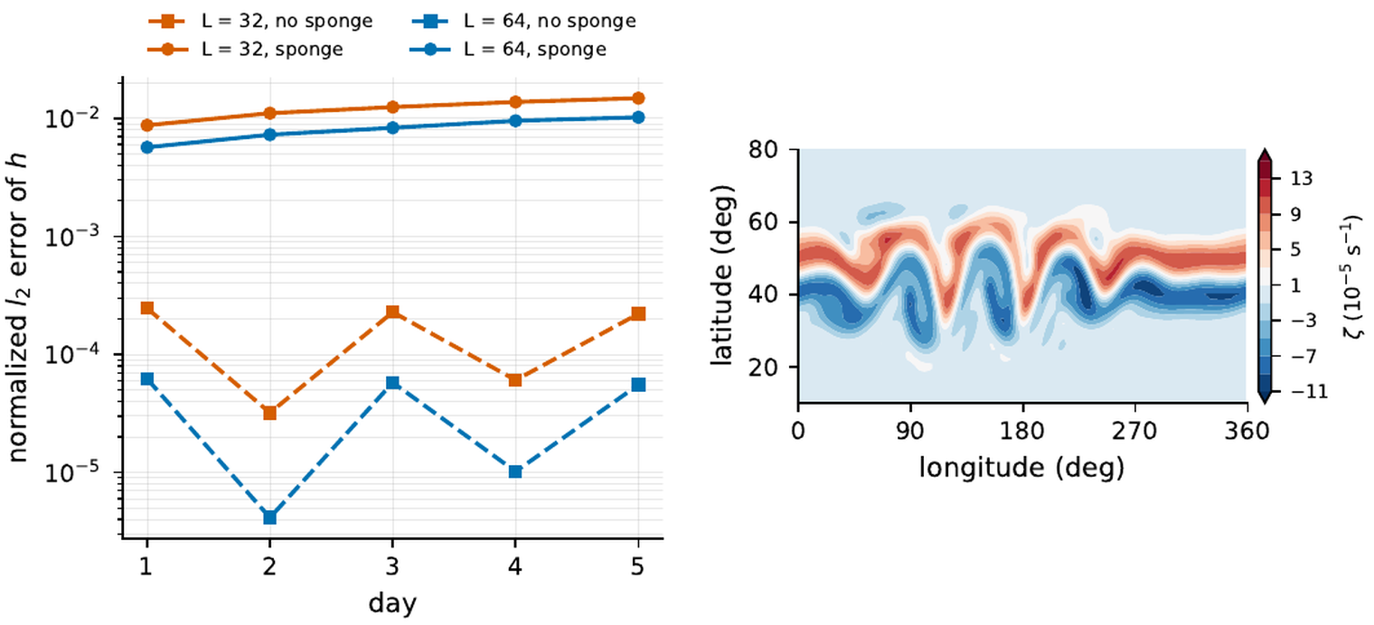
|
+
__all__ = ["SWEModel", "SphereGrid", "ZonalRelaxation", "presets", "climatology", "initial_conditions", "integrators", "dynamics", "diagnostics", "__version__"]
|
swesphere/climatology.py
ADDED
|
@@ -0,0 +1,38 @@
|
|
|
1
|
+
# -*- coding: utf-8 -*-
|
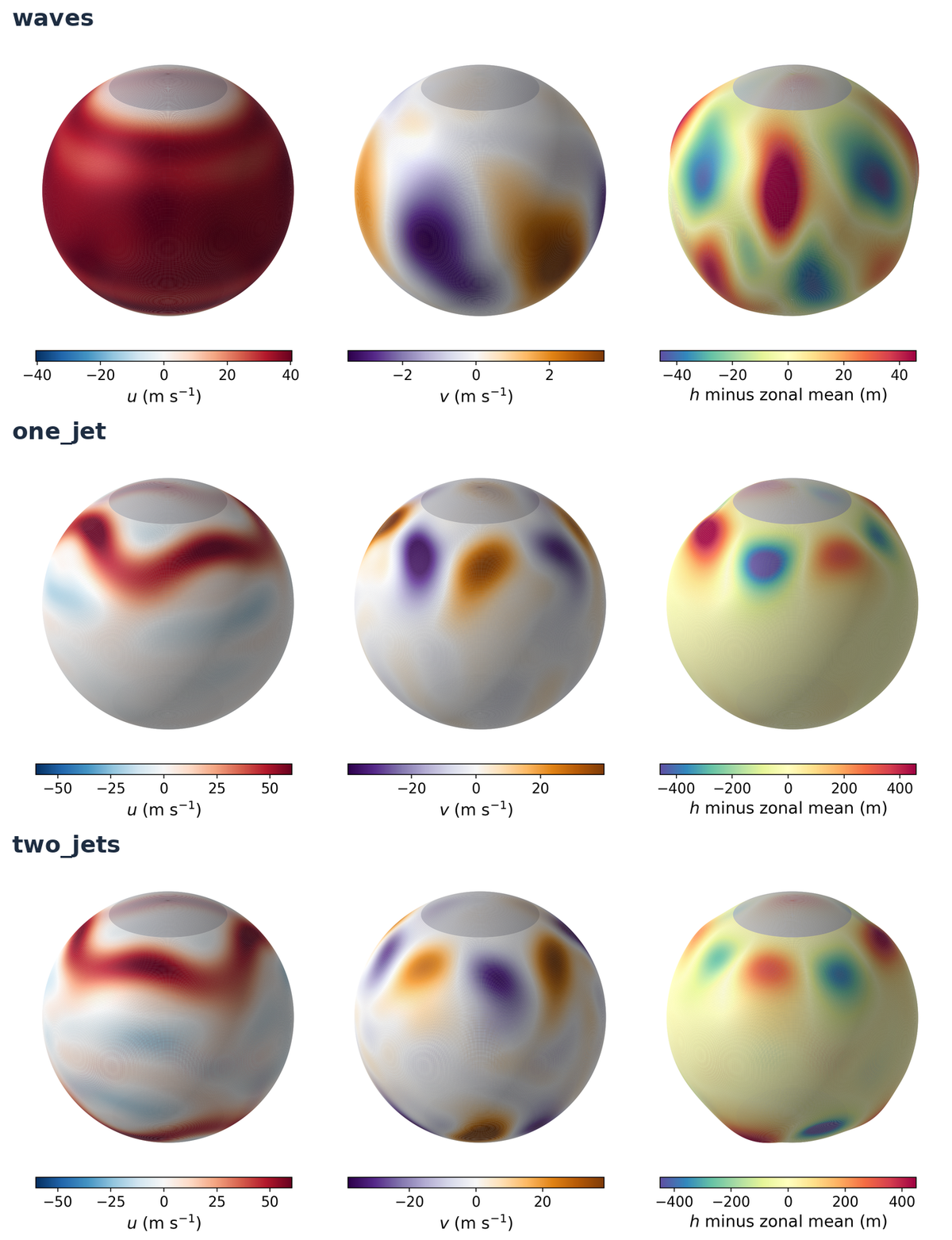
|
2
|
+
"""Climatology builder: spin-up, snapshots, decorrelation check, normalization."""
|
|
3
|
+
from __future__ import annotations
|
|
4
|
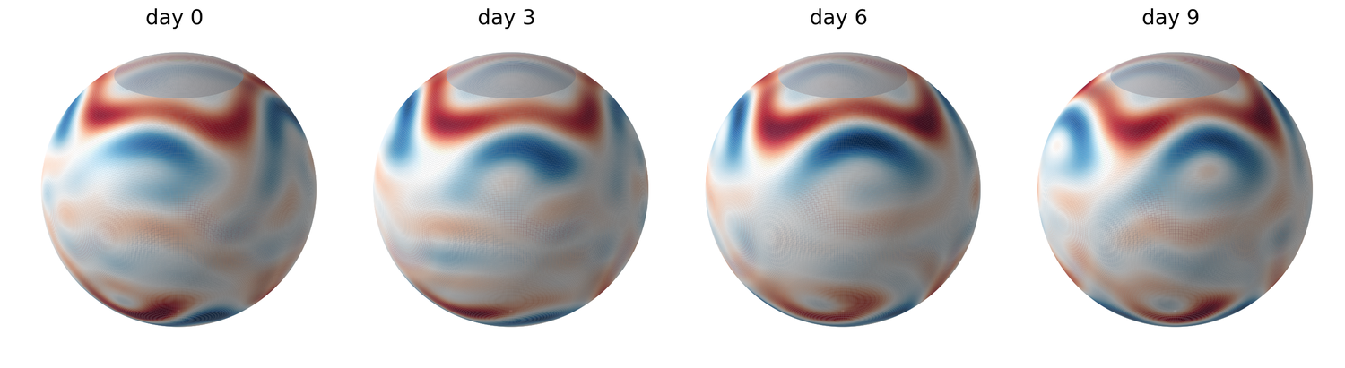
+
|
|
5
|
+
import numpy as np
|
|
6
|
+
|
|
7
|
+
DAY = 86400.0
|
|
8
|
+
|
|
9
|
+
|
|
10
|
+
def build_climatology(model, x0, spinup_days, n_snapshots, every_days, verbose=False, label=""):
|
|
11
|
+
"""Spin up ``spinup_days`` from ``x0`` and keep ``n_snapshots`` states ``every_days`` apart (float32).
|
|
12
|
+
|
|
13
|
+
For a forced preset this samples a stationary regime. For the unforced ``waves`` preset the record is a
|
|
14
|
+
slowly decaying flow (the filter is the only sink), so its early and late states differ in amplitude.
|
|
15
|
+
"""
|
|
16
|
+
if verbose:
|
|
17
|
+
print(f" {label} spin-up of {spinup_days:g} days", flush=True)
|
|
18
|
+
x = model.propagate(x0, [0.0, spinup_days * DAY])
|
|
19
|
+
if verbose:
|
|
20
|
+
print(f" {label} spin-up done", flush=True)
|
|
21
|
+
snaps = [x.astype(np.float32)]
|
|
22
|
+
for k in range(n_snapshots - 1):
|
|
23
|
+
x = model.propagate(x, [0.0, every_days * DAY]); snaps.append(x.astype(np.float32))
|
|
24
|
+
if verbose and (k + 1) % 10 == 0:
|
|
25
|
+
print(f" {label} {k + 1}/{n_snapshots} snapshots", flush=True)
|
|
26
|
+
return np.array(snaps)
|
|
27
|
+
|
|
28
|
+
|
|
29
|
+
def anomaly_scales(model, snapshots):
|
|
30
|
+
"""Per-field standard deviation of the climatological anomalies, repeated over the state."""
|
|
31
|
+
A = snapshots - snapshots.mean(axis=0); fs = model.field_size
|
|
32
|
+
sd = np.array([A[:, k * fs:(k + 1) * fs].std() for k in range(3)])
|
|
33
|
+
return np.repeat(sd, fs), sd
|
|
34
|
+
|
|
35
|
+
|
|
36
|
+
def lag_correlation(model, snapshots, lag=1, field="h"):
|
|
37
|
+
A = snapshots - snapshots.mean(axis=0); blk = model.var_blocks[field]; a = A[:, blk]
|
|
38
|
+
return float(np.mean([np.corrcoef(a[i], a[i + lag])[0, 1] for i in range(len(a) - lag)]))
|
swesphere/diagnostics.py
ADDED
|
@@ -0,0 +1,39 @@
|
|
|
1
|
+
# -*- coding: utf-8 -*-
|
|
2
|
+
"""Global invariants of the shallow-water equations and error norms.
|
|
3
|
+
|
|
4
|
+
All integrals are area weighted (cos φ) over the whole grid, or over the rows
|
|
5
|
+
outside the polar sponge with ``interior=True``. The continuous equations
|
|
6
|
+
conserve mass, total energy and potential enstrophy; the discrete model loses a
|
|
7
|
+
little of each through the spectral filter and the polar sponge, and the forced
|
|
8
|
+
presets exchange them with the relaxation. EXP-00 reports the measured drifts.
|
|
9
|
+
"""
|
|
10
|
+
from __future__ import annotations
|
|
11
|
+
|
|
12
|
+
import numpy as np
|
|
13
|
+
|
|
14
|
+
from .dynamics import relative_vorticity
|
|
15
|
+
|
|
16
|
+
|
|
17
|
+
def area_weights(model, interior: bool = False) -> np.ndarray:
|
|
18
|
+
w = np.clip(np.asarray(model.grid.cosL), 0.0, None).copy()
|
|
19
|
+
if interior:
|
|
20
|
+
k = model.n_pole_rows; w[:k] = 0.0; w[model.Nlat - k:] = 0.0
|
|
21
|
+
return w / w.sum()
|
|
22
|
+
|
|
23
|
+
|
|
24
|
+
def invariants(model, x, interior: bool = False) -> dict:
|
|
25
|
+
"""Mean depth (m), total energy per unit area (J/kg m) and potential enstrophy."""
|
|
26
|
+
u, v, h = model.unpack(np.asarray(x, dtype=float)); G = model.grid; w = area_weights(model, interior)
|
|
27
|
+
eta = relative_vorticity(u, v, G) + G.f_cor
|
|
28
|
+
return dict(mass=float((w * h).sum()),
|
|
29
|
+
energy=float((w * (0.5 * h * (u ** 2 + v ** 2) + 0.5 * G.g * h ** 2)).sum()),
|
|
30
|
+
enstrophy=float((w * 0.5 * eta ** 2 / h).sum()))
|
|
31
|
+
|
|
32
|
+
|
|
33
|
+
def error_norms(model, x, x_ref, field: str = "h", interior: bool = True) -> dict:
|
|
34
|
+
"""Normalized l1, l2 and l-infinity errors of Williamson et al. (1992)."""
|
|
35
|
+
i = "uvh".index(field); q = model.unpack(np.asarray(x, dtype=float))[i]; r = model.unpack(np.asarray(x_ref, dtype=float))[i]
|
|
36
|
+
w = area_weights(model, interior); m = w > 0
|
|
37
|
+
return dict(l1=float((w * np.abs(q - r)).sum() / (w * np.abs(r)).sum()),
|
|
38
|
+
l2=float(np.sqrt((w * (q - r) ** 2).sum() / (w * r ** 2).sum())),
|
|
39
|
+
linf=float(np.abs(q - r)[m].max() / np.abs(r)[m].max()))
|
swesphere/dynamics.py
ADDED
|
@@ -0,0 +1,88 @@
|
|
|
1
|
+
# -*- coding: utf-8 -*-
|
|
2
|
+
"""
|
|
3
|
+
Vector-invariant form of the shallow-water equations on the sphere.
|
|
4
|
+
|
|
5
|
+
State variables
|
|
6
|
+
---------------
|
|
7
|
+
* ``u(λ, φ)``, zonal velocity (m/s)
|
|
8
|
+
* ``v(λ, φ)``, meridional velocity (m/s)
|
|
9
|
+
* ``h(λ, φ)``, layer thickness (m)
|
|
10
|
+
|
|
11
|
+
Equations (Hack & Jakob 1992 form)
|
|
12
|
+
----------------------------------
|
|
13
|
+
∂u/∂t = η v − (1 / a cosφ) ∂B/∂λ
|
|
14
|
+
∂v/∂t = −η u − (1 / a) ∂B/∂φ
|
|
15
|
+
∂h/∂t = −∇·(h V) = −(1 / a cosφ) [∂(h u)/∂λ + ∂(h v cosφ)/∂φ]
|
|
16
|
+
|
|
17
|
+
where:
|
|
18
|
+
ζ = (1 / a cosφ) ∂v/∂λ − (1/a) ∂u/∂φ + (tanφ/a) u (relative vorticity)
|
|
19
|
+
η = ζ + f (absolute vorticity)
|
|
20
|
+
B = g h + ½(u² + v²) (Bernoulli potential)
|
|
21
|
+
δ = (1 / a cosφ) ∂u/∂λ + (1 / a cosφ) ∂(v cosφ)/∂φ (divergence, diagnostic only)
|
|
22
|
+
|
|
23
|
+
The continuity equation is discretized in flux form, so the zonal FFT derivative and
|
|
24
|
+
the centered meridional difference telescope and the global mass changes only through
|
|
25
|
+
the spectral filter and the polar rows. (Versions before 0.2.0 used ``dh = -h δ`` and
|
|
26
|
+
omitted the advection of ``h``; see CHANGELOG.md.)
|
|
27
|
+
"""
|
|
28
|
+
|
|
29
|
+
from __future__ import annotations
|
|
30
|
+
|
|
31
|
+
from typing import Tuple
|
|
32
|
+
|
|
33
|
+
import numpy as np
|
|
34
|
+
|
|
35
|
+
from .grid import SphereGrid, d_lon, d_lat
|
|
36
|
+
|
|
37
|
+
|
|
38
|
+
def rhs(
|
|
39
|
+
u: np.ndarray,
|
|
40
|
+
v: np.ndarray,
|
|
41
|
+
h: np.ndarray,
|
|
42
|
+
grid: SphereGrid,
|
|
43
|
+
) -> Tuple[np.ndarray, np.ndarray, np.ndarray]:
|
|
44
|
+
"""Return ``(du/dt, dv/dt, dh/dt)`` for the SWE system."""
|
|
45
|
+
cos = grid.cos_safe
|
|
46
|
+
a = grid.a
|
|
47
|
+
|
|
48
|
+
# Relative vorticity ζ
|
|
49
|
+
zeta = (d_lon(v, grid) / (a * cos)
|
|
50
|
+
- d_lat(u, grid) / a
|
|
51
|
+
+ grid.sinL / cos * u / a)
|
|
52
|
+
|
|
53
|
+
# Absolute vorticity η
|
|
54
|
+
eta = zeta + grid.f_cor
|
|
55
|
+
|
|
56
|
+
# Bernoulli potential
|
|
57
|
+
B = grid.g * h + 0.5 * (u ** 2 + v ** 2)
|
|
58
|
+
|
|
59
|
+
# Tendencies: vector-invariant momentum, flux-form continuity
|
|
60
|
+
du = eta * v - d_lon(B, grid) / (a * cos)
|
|
61
|
+
dv = -eta * u - d_lat(B, grid) / a
|
|
62
|
+
dh = -(d_lon(h * u, grid) + d_lat(h * v * grid.cosL, grid)) / (a * cos)
|
|
63
|
+
|
|
64
|
+
return du, dv, dh
|
|
65
|
+
|
|
66
|
+
|
|
67
|
+
def relative_vorticity(u: np.ndarray, v: np.ndarray,
|
|
68
|
+
grid: SphereGrid) -> np.ndarray:
|
|
69
|
+
"""Diagnostic: relative vorticity ζ from (u, v)."""
|
|
70
|
+
cos = grid.cos_safe
|
|
71
|
+
a = grid.a
|
|
72
|
+
return (d_lon(v, grid) / (a * cos)
|
|
73
|
+
- d_lat(u, grid) / a
|
|
74
|
+
+ grid.sinL / cos * u / a)
|
|
75
|
+
|
|
76
|
+
|
|
77
|
+
def divergence(u: np.ndarray, v: np.ndarray,
|
|
78
|
+
grid: SphereGrid) -> np.ndarray:
|
|
79
|
+
"""Diagnostic: horizontal divergence δ from (u, v)."""
|
|
80
|
+
cos = grid.cos_safe
|
|
81
|
+
a = grid.a
|
|
82
|
+
return (d_lon(u, grid) / (a * cos)
|
|
83
|
+
+ d_lat(v * grid.cosL, grid) / (a * cos))
|
|
84
|
+
|
|
85
|
+
|
|
86
|
+
def divergence(u: np.ndarray, v: np.ndarray, grid: SphereGrid) -> np.ndarray:
|
|
87
|
+
"""Diagnostic: horizontal divergence δ from (u, v)."""
|
|
88
|
+
return (d_lon(u, grid) + d_lat(v * grid.cosL, grid)) / (grid.a * grid.cos_safe)
|
swesphere/forcing.py
ADDED
|
@@ -0,0 +1,26 @@
|
|
|
1
|
+
# -*- coding: utf-8 -*-
|
|
2
|
+
"""Forcing that gives the model a stationary turbulent regime.
|
|
3
|
+
|
|
4
|
+
Without forcing the shallow-water equations on the sphere do not sustain eddies: the filter dissipates
|
|
5
|
+
whatever the initial condition put in and the flow relaxes toward a zonal state with weak, slowly
|
|
6
|
+
decaying waves (the ``waves`` preset). ``ZonalRelaxation`` relaxes only the zonal mean of (u, v, h)
|
|
7
|
+
toward a reference jet and leaves the eddies alone; with a barotropically unstable reference
|
|
8
|
+
(Galewsky) the instability regenerates eddies against the dissipation and the flow reaches a
|
|
9
|
+
stationary turbulent state (EXP-02 measures its statistics). Relaxing the full fields toward the
|
|
10
|
+
zonal state kills the eddies instead.
|
|
11
|
+
"""
|
|
12
|
+
from __future__ import annotations
|
|
13
|
+
|
|
14
|
+
import numpy as np
|
|
15
|
+
|
|
16
|
+
|
|
17
|
+
class ZonalRelaxation:
|
|
18
|
+
def __init__(self, u_ref, v_ref, h_ref, tau):
|
|
19
|
+
self.k = 1.0 / float(tau)
|
|
20
|
+
self.ref = tuple(np.repeat(np.asarray(f).mean(axis=1, keepdims=True), np.asarray(f).shape[1], axis=1) for f in (u_ref, v_ref, h_ref))
|
|
21
|
+
|
|
22
|
+
def __call__(self, u, v, h, du, dv, dh):
|
|
23
|
+
for f, r_, d_ in ((u, self.ref[0], du), (v, self.ref[1], dv), (h, self.ref[2], dh)):
|
|
24
|
+
zm = np.repeat(f.mean(axis=1, keepdims=True), f.shape[1], axis=1)
|
|
25
|
+
d_ -= self.k * (zm - r_)
|
|
26
|
+
return du, dv, dh
|
swesphere/grid.py
ADDED
|
@@ -0,0 +1,161 @@
|
|
|
1
|
+
# -*- coding: utf-8 -*-
|
|
2
|
+
"""
|
|
3
|
+
Driscoll-Healy spherical grid and numerical operators.
|
|
4
|
+
|
|
5
|
+
Geometry
|
|
6
|
+
--------
|
|
7
|
+
* Grid is stored North-to-South with `Nlat = 2*(LMAX+1)` rows and
|
|
8
|
+
`Nlon = 4*(LMAX+1)` columns.
|
|
9
|
+
* Latitudes range from +90° (row 0) down to -90° (row Nlat-1), exclusive
|
|
10
|
+
of the south pole (DH convention).
|
|
11
|
+
* Longitudes are equally spaced 0 to 360°, exclusive of 360.
|
|
12
|
+
|
|
13
|
+
Operators
|
|
14
|
+
---------
|
|
15
|
+
* ``d_lon(q)``, exact zonal derivative via FFT.
|
|
16
|
+
* ``d_lat(q)``, centered finite-difference meridional derivative
|
|
17
|
+
(with sign flip for N→S storage).
|
|
18
|
+
* ``sh_filter(q, alpha, p)``, exponential filter in spherical harmonics:
|
|
19
|
+
attenuates degree n by ``exp(-alpha * (n/Lmax)^p)``. Removes aliasing
|
|
20
|
+
and polar noise.
|
|
21
|
+
* ``make_sponge(...)``, multiplicative damping near the poles.
|
|
22
|
+
"""
|
|
23
|
+
|
|
24
|
+
from __future__ import annotations
|
|
25
|
+
|
|
26
|
+
from dataclasses import dataclass
|
|
27
|
+
from typing import Tuple
|
|
28
|
+
|
|
29
|
+
import numpy as np
|
|
30
|
+
|
|
31
|
+
import pyshtools as pysh
|
|
32
|
+
|
|
33
|
+
|
|
34
|
+
# ----------------------------------------------------------------------
|
|
35
|
+
# Grid
|
|
36
|
+
# ----------------------------------------------------------------------
|
|
37
|
+
@dataclass
|
|
38
|
+
class SphereGrid:
|
|
39
|
+
"""Driscoll-Healy spherical grid metadata.
|
|
40
|
+
|
|
41
|
+
Attributes
|
|
42
|
+
----------
|
|
43
|
+
LMAX : int
|
|
44
|
+
Spectral truncation (T-LMAX).
|
|
45
|
+
Nlat, Nlon : int
|
|
46
|
+
Grid dimensions in latitude and longitude.
|
|
47
|
+
a : float
|
|
48
|
+
Earth radius (m).
|
|
49
|
+
Omega : float
|
|
50
|
+
Earth angular velocity (rad/s).
|
|
51
|
+
g : float
|
|
52
|
+
Gravitational acceleration (m/s^2).
|
|
53
|
+
LON_ns, LAT_ns : ndarray
|
|
54
|
+
Meshgrids of longitude and latitude in radians, stored N→S.
|
|
55
|
+
cosL, sinL, f_cor : ndarray
|
|
56
|
+
Geometric quantities (cos φ, sin φ, Coriolis parameter).
|
|
57
|
+
cos_safe : ndarray
|
|
58
|
+
cos φ with a small minimum value to avoid polar singularity.
|
|
59
|
+
kx : ndarray
|
|
60
|
+
Zonal wavenumbers for FFT.
|
|
61
|
+
dlat : float
|
|
62
|
+
Meridional grid spacing in radians.
|
|
63
|
+
"""
|
|
64
|
+
LMAX: int
|
|
65
|
+
Nlat: int
|
|
66
|
+
Nlon: int
|
|
67
|
+
a: float
|
|
68
|
+
Omega: float
|
|
69
|
+
g: float
|
|
70
|
+
LON_ns: np.ndarray
|
|
71
|
+
LAT_ns: np.ndarray
|
|
72
|
+
cosL: np.ndarray
|
|
73
|
+
sinL: np.ndarray
|
|
74
|
+
f_cor: np.ndarray
|
|
75
|
+
cos_safe: np.ndarray
|
|
76
|
+
kx: np.ndarray
|
|
77
|
+
dlat: float
|
|
78
|
+
|
|
79
|
+
@classmethod
|
|
80
|
+
def make(
|
|
81
|
+
cls,
|
|
82
|
+
LMAX: int = 32,
|
|
83
|
+
a: float = 6.371e6,
|
|
84
|
+
Omega: float = 7.292e-5,
|
|
85
|
+
g: float = 9.81,
|
|
86
|
+
cos_floor: float = 0.08,
|
|
87
|
+
) -> "SphereGrid":
|
|
88
|
+
Nlat = 2 * (LMAX + 1)
|
|
89
|
+
Nlon = 4 * (LMAX + 1)
|
|
90
|
+
lats = 90 - np.arange(Nlat) * 180 / Nlat # degrees, N→S
|
|
91
|
+
lons = np.arange(Nlon) * 360 / Nlon
|
|
92
|
+
LON_ns, LAT_ns = np.meshgrid(np.radians(lons), np.radians(lats))
|
|
93
|
+
cosL = np.cos(LAT_ns)
|
|
94
|
+
sinL = np.sin(LAT_ns)
|
|
95
|
+
f_cor = 2 * Omega * sinL
|
|
96
|
+
cos_safe = np.where(np.abs(cosL) < cos_floor,
|
|
97
|
+
np.sign(cosL + 1e-10) * cos_floor, cosL)
|
|
98
|
+
kx = np.fft.rfftfreq(Nlon, d=1.0 / Nlon)
|
|
99
|
+
dlat = np.radians(180 / Nlat)
|
|
100
|
+
return cls(LMAX=LMAX, Nlat=Nlat, Nlon=Nlon, a=a, Omega=Omega, g=g,
|
|
101
|
+
LON_ns=LON_ns, LAT_ns=LAT_ns, cosL=cosL, sinL=sinL,
|
|
102
|
+
f_cor=f_cor, cos_safe=cos_safe, kx=kx, dlat=dlat)
|
|
103
|
+
|
|
104
|
+
|
|
105
|
+
# ----------------------------------------------------------------------
|
|
106
|
+
# Operators
|
|
107
|
+
# ----------------------------------------------------------------------
|
|
108
|
+
def d_lon(q: np.ndarray, grid: SphereGrid) -> np.ndarray:
|
|
109
|
+
"""Exact zonal derivative ∂q/∂λ via FFT."""
|
|
110
|
+
return np.fft.irfft(1j * grid.kx * np.fft.rfft(q, axis=1),
|
|
111
|
+
n=grid.Nlon, axis=1)
|
|
112
|
+
|
|
113
|
+
|
|
114
|
+
def d_lat(q: np.ndarray, grid: SphereGrid) -> np.ndarray:
|
|
115
|
+
"""Centered finite-difference meridional derivative ∂q/∂φ.
|
|
116
|
+
|
|
117
|
+
The grid is stored N→S, so dq/d(row index) has opposite sign to
|
|
118
|
+
dq/d(latitude), we flip the sign.
|
|
119
|
+
"""
|
|
120
|
+
dq = np.zeros_like(q)
|
|
121
|
+
dq[1:-1] = (q[2:] - q[:-2]) / (2 * grid.dlat)
|
|
122
|
+
dq[0] = (q[1] - q[0]) / grid.dlat
|
|
123
|
+
dq[-1] = (q[-1] - q[-2]) / grid.dlat
|
|
124
|
+
return -dq
|
|
125
|
+
|
|
126
|
+
|
|
127
|
+
def sh_filter(
|
|
128
|
+
q: np.ndarray,
|
|
129
|
+
grid: SphereGrid,
|
|
130
|
+
alpha: float = 36.0,
|
|
131
|
+
p: int = 16,
|
|
132
|
+
) -> np.ndarray:
|
|
133
|
+
"""Exponential filter in spherical harmonics.
|
|
134
|
+
|
|
135
|
+
Attenuates spherical-harmonic degree ``n`` by ``exp(-alpha*(n/LMAX)^p)``.
|
|
136
|
+
With ``p=16`` this is essentially a brick-wall filter that passes
|
|
137
|
+
``n < LMAX`` and cuts ``n ~ LMAX``. Removes aliasing and polar noise
|
|
138
|
+
that builds up under explicit time integration.
|
|
139
|
+
"""
|
|
140
|
+
L = grid.LMAX
|
|
141
|
+
c = pysh.expand.SHExpandDH(q, norm=1, sampling=2, lmax_calc=L)
|
|
142
|
+
n_arr = np.arange(L + 1)
|
|
143
|
+
decay = np.exp(-alpha * (n_arr / max(L, 1)) ** p)
|
|
144
|
+
c = c * decay[None, :, None]
|
|
145
|
+
return pysh.expand.MakeGridDH(c, norm=1, sampling=2, lmax=L)
|
|
146
|
+
|
|
147
|
+
|
|
148
|
+
def make_sponge(Nlat: int, n_pole_rows: int = 10,
|
|
149
|
+
strength: float = 0.98) -> np.ndarray:
|
|
150
|
+
"""Build a multiplicative damping mask near the poles.
|
|
151
|
+
|
|
152
|
+
Returns an array of shape ``(Nlat, 1)`` that is < 1 within
|
|
153
|
+
``n_pole_rows`` of each pole, ramping linearly from full damping
|
|
154
|
+
(``1 - strength``) at the pole to 1 at the edge of the sponge band.
|
|
155
|
+
"""
|
|
156
|
+
sponge = np.ones((Nlat, 1))
|
|
157
|
+
for i in range(n_pole_rows):
|
|
158
|
+
w = (n_pole_rows - i) / n_pole_rows * strength
|
|
159
|
+
sponge[i] = 1 - w
|
|
160
|
+
sponge[-1 - i] = 1 - w
|
|
161
|
+
return sponge
|
|
@@ -0,0 +1,160 @@
|
|
|
1
|
+
# -*- coding: utf-8 -*-
|
|
2
|
+
"""
|
|
3
|
+
Initial conditions for the SWE on the sphere.
|
|
4
|
+
|
|
5
|
+
Two ingredients:
|
|
6
|
+
|
|
7
|
+
* **Solid-body rotation** (Williamson et al. 1992, Test Case 2). An
|
|
8
|
+
exact stationary solution of the SWE on the sphere::
|
|
9
|
+
|
|
10
|
+
u = U0 · cos φ
|
|
11
|
+
v = 0
|
|
12
|
+
h = H0 − (a Ω U0 + U0² / 2) / g · sin² φ
|
|
13
|
+
|
|
14
|
+
The default base state of every IC.
|
|
15
|
+
|
|
16
|
+
* **Rossby-wave perturbations** in each hemisphere, gaussian-enveloped
|
|
17
|
+
in latitude and zonally sinusoidal::
|
|
18
|
+
|
|
19
|
+
δh = A_h · cos(k λ) · exp(−(φ − φ₀)² / (2 σ²))
|
|
20
|
+
δu = A_uv · cos(k λ) · exp(...)
|
|
21
|
+
δv = A_uv · sin(k λ) · exp(...)
|
|
22
|
+
|
|
23
|
+
Default amplitudes and shapes match the reference setup from the
|
|
24
|
+
upstream visualization script.
|
|
25
|
+
"""
|
|
26
|
+
|
|
27
|
+
from __future__ import annotations
|
|
28
|
+
|
|
29
|
+
from dataclasses import dataclass, field
|
|
30
|
+
from typing import Tuple
|
|
31
|
+
|
|
32
|
+
import numpy as np
|
|
33
|
+
|
|
34
|
+
from .grid import SphereGrid
|
|
35
|
+
|
|
36
|
+
|
|
37
|
+
@dataclass
|
|
38
|
+
class RossbyPert:
|
|
39
|
+
"""Rossby-wave-like perturbation envelope and amplitudes."""
|
|
40
|
+
amp_h: float = 220.0 # Amplitude in h (m)
|
|
41
|
+
amp_uv: float = 6.0 # Amplitude in (u, v) (m/s)
|
|
42
|
+
wavenumber: int = 4 # Zonal wavenumber
|
|
43
|
+
lat_center: float = 42.0 # Latitude of the gaussian center (deg)
|
|
44
|
+
width: float = 12.0 # Gaussian width (deg)
|
|
45
|
+
phase: float = 0.0 # Phase offset (rad)
|
|
46
|
+
|
|
47
|
+
|
|
48
|
+
def williamson_tc2(grid: SphereGrid, U0: float = 38.0,
|
|
49
|
+
H0: float = 2800.0
|
|
50
|
+
) -> Tuple[np.ndarray, np.ndarray, np.ndarray]:
|
|
51
|
+
"""Williamson 1992 Test Case 2: solid-body rotation."""
|
|
52
|
+
u = U0 * grid.cosL
|
|
53
|
+
v = np.zeros_like(u)
|
|
54
|
+
h = H0 - (grid.a * grid.Omega * U0 + 0.5 * U0 ** 2) / grid.g * grid.sinL ** 2
|
|
55
|
+
return u, v, h
|
|
56
|
+
|
|
57
|
+
|
|
58
|
+
def add_rossby_perturbation(
|
|
59
|
+
u: np.ndarray, v: np.ndarray, h: np.ndarray,
|
|
60
|
+
grid: SphereGrid, pert: RossbyPert,
|
|
61
|
+
):
|
|
62
|
+
"""Add a single Rossby-wave perturbation in-place."""
|
|
63
|
+
phi0 = np.radians(pert.lat_center)
|
|
64
|
+
sigma = np.radians(pert.width)
|
|
65
|
+
env = np.exp(-((grid.LAT_ns - phi0) ** 2) / (2 * sigma ** 2))
|
|
66
|
+
cos_arg = pert.wavenumber * grid.LON_ns + pert.phase
|
|
67
|
+
sin_arg = pert.wavenumber * grid.LON_ns + pert.phase
|
|
68
|
+
h += pert.amp_h * np.cos(cos_arg) * env
|
|
69
|
+
u += pert.amp_uv * np.cos(cos_arg) * env
|
|
70
|
+
v += pert.amp_uv * np.sin(sin_arg) * env
|
|
71
|
+
|
|
72
|
+
|
|
73
|
+
def default_ic(grid: SphereGrid, U0: float = 38.0,
|
|
74
|
+
H0: float = 2800.0
|
|
75
|
+
) -> Tuple[np.ndarray, np.ndarray, np.ndarray]:
|
|
76
|
+
"""Default IC: TC2 + NH wavenumber-4 + SH wavenumber-3 perturbations."""
|
|
77
|
+
u, v, h = williamson_tc2(grid, U0=U0, H0=H0)
|
|
78
|
+
add_rossby_perturbation(u, v, h, grid, RossbyPert(
|
|
79
|
+
amp_h=220.0, amp_uv=6.0, wavenumber=4,
|
|
80
|
+
lat_center=42.0, width=12.0, phase=0.0,
|
|
81
|
+
))
|
|
82
|
+
add_rossby_perturbation(u, v, h, grid, RossbyPert(
|
|
83
|
+
amp_h=150.0, amp_uv=0.0, wavenumber=3,
|
|
84
|
+
lat_center=-38.0, width=11.0, phase=1.1,
|
|
85
|
+
))
|
|
86
|
+
# Small extra meridional component on the SH band, matching the
|
|
87
|
+
# reference setup (proportional to amp_h / 50 in the original).
|
|
88
|
+
phi2 = np.radians(-38.0)
|
|
89
|
+
env2 = np.exp(-((grid.LAT_ns - phi2) ** 2) / (2 * np.radians(11.0) ** 2))
|
|
90
|
+
v += (150.0 / 50) * np.sin(3 * grid.LON_ns + 1.1) * env2
|
|
91
|
+
return u, v, h
|
|
92
|
+
|
|
93
|
+
|
|
94
|
+
def perturbed_ic(
|
|
95
|
+
grid: SphereGrid,
|
|
96
|
+
seed: int = 0,
|
|
97
|
+
U0: float = 38.0,
|
|
98
|
+
H0: float = 2800.0,
|
|
99
|
+
pert_strength: float = 0.05,
|
|
100
|
+
) -> Tuple[np.ndarray, np.ndarray, np.ndarray]:
|
|
101
|
+
"""Default IC plus a small random perturbation of ``u`` and ``h`` at zonal wavenumbers 1-8,
|
|
102
|
+
confined to low and middle latitudes, to start runs from different states.
|
|
103
|
+
|
|
104
|
+
The perturbations of ``u`` and ``h`` have independent phases, so they are not in geostrophic
|
|
105
|
+
balance: they excite weak gravity waves that the model radiates and filters within a few days.
|
|
106
|
+
Use a spin-up before sampling.
|
|
107
|
+
"""
|
|
108
|
+
u, v, h = default_ic(grid, U0=U0, H0=H0)
|
|
109
|
+
rng = np.random.default_rng(seed)
|
|
110
|
+
|
|
111
|
+
# Low zonal wavenumbers, gaussian envelope in latitude.
|
|
112
|
+
Nlon = grid.Nlon
|
|
113
|
+
n_modes = 8
|
|
114
|
+
for k in range(1, n_modes + 1):
|
|
115
|
+
amp_u = pert_strength * U0 * rng.standard_normal()
|
|
116
|
+
amp_h = pert_strength * H0 * 0.05 * rng.standard_normal()
|
|
117
|
+
phase_u = 2 * np.pi * rng.random()
|
|
118
|
+
phase_h = 2 * np.pi * rng.random()
|
|
119
|
+
# Latitude-banded modulation
|
|
120
|
+
lat_mod = np.exp(-(grid.LAT_ns / np.radians(45.0)) ** 2)
|
|
121
|
+
u += amp_u * np.cos(k * grid.LON_ns + phase_u) * lat_mod
|
|
122
|
+
h += amp_h * np.cos(k * grid.LON_ns + phase_h) * lat_mod
|
|
123
|
+
return u, v, h
|
|
124
|
+
|
|
125
|
+
|
|
126
|
+
# ---------------------------------------------------------------------------
|
|
127
|
+
# Galewsky, Scott & Polvani (2004): a balanced, barotropically unstable jet
|
|
128
|
+
# ---------------------------------------------------------------------------
|
|
129
|
+
def galewsky_jet(grid: SphereGrid, umax: float = 80.0, phi0_deg: float = 25.7, phi1_deg: float = 64.6,
|
|
130
|
+
h0: float = 10000.0, bump: bool = True, both_hemispheres: bool = True):
|
|
131
|
+
"""Balanced zonal jet(s) with the small height bump that triggers the instability.
|
|
132
|
+
|
|
133
|
+
Returns ``(u, v, h)`` on the grid. With ``both_hemispheres`` a mirror jet
|
|
134
|
+
(also westerly) is placed in the south so the whole sphere is active; the
|
|
135
|
+
two hemispheres perturb each other across the equator and the resulting
|
|
136
|
+
turbulence is irregular (with the zonal relaxation of :mod:`swesphere.forcing`).
|
|
137
|
+
"""
|
|
138
|
+
Nlat, Nlon = grid.Nlat, grid.Nlon
|
|
139
|
+
lats = np.radians(90 - np.arange(Nlat) * 180 / Nlat); lons = np.radians(np.arange(Nlon) * 360 / Nlon)
|
|
140
|
+
phi0, phi1 = np.radians(phi0_deg), np.radians(phi1_deg); en = np.exp(-4.0 / (phi1 - phi0) ** 2)
|
|
141
|
+
|
|
142
|
+
def uprof(phi):
|
|
143
|
+
out = np.zeros_like(phi); m = (phi > phi0) & (phi < phi1)
|
|
144
|
+
out[m] = umax / en * np.exp(1.0 / ((phi[m] - phi0) * (phi[m] - phi1)))
|
|
145
|
+
if both_hemispheres:
|
|
146
|
+
ms = (-phi > phi0) & (-phi < phi1)
|
|
147
|
+
out[ms] = umax / en * np.exp(1.0 / ((-phi[ms] - phi0) * (-phi[ms] - phi1)))
|
|
148
|
+
return out
|
|
149
|
+
|
|
150
|
+
fine = np.linspace(-np.pi / 2, np.pi / 2, 4001); uf = uprof(fine); f = 2 * grid.Omega * np.sin(fine)
|
|
151
|
+
dh = -grid.a * uf * (f + uf * np.tan(fine) / grid.a) / grid.g
|
|
152
|
+
hf = np.concatenate([[0.0], np.cumsum(0.5 * (dh[1:] + dh[:-1]) * np.diff(fine))]); hf = h0 + hf - hf.mean()
|
|
153
|
+
u = np.repeat(uprof(lats)[:, None], Nlon, axis=1); v = np.zeros_like(u)
|
|
154
|
+
h = np.repeat(np.interp(lats, fine, hf)[:, None], Nlon, axis=1)
|
|
155
|
+
if bump:
|
|
156
|
+
LON, LAT = np.meshgrid(lons, lats); phi2 = np.pi / 4; alpha, beta = 1 / 3, 1 / 15
|
|
157
|
+
h = h + 120.0 * np.cos(LAT) * np.exp(-((LON - np.pi) / alpha) ** 2) * np.exp(-((phi2 - LAT) / beta) ** 2)
|
|
158
|
+
if both_hemispheres:
|
|
159
|
+
h = h + 120.0 * np.cos(LAT) * np.exp(-((LON - 0.4 * np.pi) / alpha) ** 2) * np.exp(-((-phi2 - LAT) / beta) ** 2)
|
|
160
|
+
return u, v, h
|
swesphere/integrators.py
ADDED
|
@@ -0,0 +1,22 @@
|
|
|
1
|
+
# -*- coding: utf-8 -*-
|
|
2
|
+
"""Time stepper for the shallow-water right-hand side: fourth-order Runge-Kutta.
|
|
3
|
+
|
|
4
|
+
RK4 with the spectral filter and the polar sponge integrates every preset for hundreds of days at
|
|
5
|
+
dt = 120 s. EXP-01 in ``experiments/`` measures the stable range of dt (a property of this scheme
|
|
6
|
+
against the fastest gravity waves; another scheme has another range) and how the eddy amplitude
|
|
7
|
+
depends on the filter cadence.
|
|
8
|
+
"""
|
|
9
|
+
from __future__ import annotations
|
|
10
|
+
|
|
11
|
+
|
|
12
|
+
def rk4(rhs, u, v, h, dt):
|
|
13
|
+
k1 = rhs(u, v, h)
|
|
14
|
+
k2 = rhs(u + 0.5 * dt * k1[0], v + 0.5 * dt * k1[1], h + 0.5 * dt * k1[2])
|
|
15
|
+
k3 = rhs(u + 0.5 * dt * k2[0], v + 0.5 * dt * k2[1], h + 0.5 * dt * k2[2])
|
|
16
|
+
k4 = rhs(u + dt * k3[0], v + dt * k3[1], h + dt * k3[2])
|
|
17
|
+
return (u + dt / 6 * (k1[0] + 2 * k2[0] + 2 * k3[0] + k4[0]),
|
|
18
|
+
v + dt / 6 * (k1[1] + 2 * k2[1] + 2 * k3[1] + k4[1]),
|
|
19
|
+
h + dt / 6 * (k1[2] + 2 * k2[2] + 2 * k3[2] + k4[2]))
|
|
20
|
+
|
|
21
|
+
|
|
22
|
+
INTEGRATORS = {"rk4": rk4}
|
swesphere/model.py
ADDED
|
@@ -0,0 +1,89 @@
|
|
|
1
|
+
# -*- coding: utf-8 -*-
|
|
2
|
+
"""The shallow-water model on the sphere with a state-vector API.
|
|
3
|
+
|
|
4
|
+
State layout: ``x = [u.ravel(), v.ravel(), h.ravel()]`` on the ``(Nlat, Nlon)``
|
|
5
|
+
grid, row-major, rows from north to south. ``field_size = Nlat * Nlon``.
|
|
6
|
+
"""
|
|
7
|
+
from __future__ import annotations
|
|
8
|
+
|
|
9
|
+
import numpy as np
|
|
10
|
+
|
|
11
|
+
from .grid import SphereGrid, sh_filter, make_sponge
|
|
12
|
+
from .dynamics import rhs as _rhs
|
|
13
|
+
from .integrators import INTEGRATORS
|
|
14
|
+
from . import initial_conditions as ics
|
|
15
|
+
|
|
16
|
+
|
|
17
|
+
class SWEModel:
|
|
18
|
+
def __init__(self, LMAX: int = 32, dt: float = 120.0, scheme: str = "rk4",
|
|
19
|
+
filter_every: int = 3, filter_alpha: float = 36.0, filter_p: int = 16,
|
|
20
|
+
n_pole_rows: int = 10, forcing=None, a: float = 6.371e6, Omega: float = 7.292e-5, g: float = 9.81):
|
|
21
|
+
self.grid = SphereGrid.make(LMAX=LMAX, a=a, Omega=Omega, g=g)
|
|
22
|
+
self.dt, self.scheme = float(dt), scheme
|
|
23
|
+
self.filter_every, self.filter_alpha, self.filter_p = int(filter_every), float(filter_alpha), int(filter_p)
|
|
24
|
+
self.n_pole_rows = int(n_pole_rows)
|
|
25
|
+
self._sponge = make_sponge(self.grid.Nlat, n_pole_rows=n_pole_rows)
|
|
26
|
+
self.forcing = forcing
|
|
27
|
+
self._step = INTEGRATORS[scheme]
|
|
28
|
+
|
|
29
|
+
# ---- layout
|
|
30
|
+
@property
|
|
31
|
+
def Nlat(self): return self.grid.Nlat
|
|
32
|
+
@property
|
|
33
|
+
def Nlon(self): return self.grid.Nlon
|
|
34
|
+
@property
|
|
35
|
+
def field_size(self): return self.grid.Nlat * self.grid.Nlon
|
|
36
|
+
@property
|
|
37
|
+
def dim(self): return 3 * self.field_size
|
|
38
|
+
@property
|
|
39
|
+
def var_blocks(self):
|
|
40
|
+
fs = self.field_size
|
|
41
|
+
return {"u": slice(0, fs), "v": slice(fs, 2 * fs), "h": slice(2 * fs, 3 * fs)}
|
|
42
|
+
|
|
43
|
+
def pack(self, u, v, h):
|
|
44
|
+
return np.concatenate([np.asarray(u).ravel(), np.asarray(v).ravel(), np.asarray(h).ravel()])
|
|
45
|
+
|
|
46
|
+
def unpack(self, x):
|
|
47
|
+
fs = self.field_size; s = (self.Nlat, self.Nlon)
|
|
48
|
+
return x[:fs].reshape(s), x[fs:2 * fs].reshape(s), x[2 * fs:3 * fs].reshape(s)
|
|
49
|
+
|
|
50
|
+
def interior_mask(self):
|
|
51
|
+
"""Boolean over one field: True outside the polar sponge (the estimated points)."""
|
|
52
|
+
rows = np.repeat(np.arange(self.Nlat), self.Nlon)
|
|
53
|
+
return (rows >= self.n_pole_rows) & (rows < self.Nlat - self.n_pole_rows)
|
|
54
|
+
|
|
55
|
+
# ---- dynamics
|
|
56
|
+
def rhs(self, u, v, h):
|
|
57
|
+
du, dv, dh = _rhs(u, v, h, self.grid)
|
|
58
|
+
if self.forcing is not None:
|
|
59
|
+
du, dv, dh = self.forcing(u, v, h, du, dv, dh)
|
|
60
|
+
return du, dv, dh
|
|
61
|
+
|
|
62
|
+
def propagate(self, x0, T, just_final_state=True):
|
|
63
|
+
if not just_final_state:
|
|
64
|
+
raise NotImplementedError
|
|
65
|
+
u, v, h = (f.copy() for f in self.unpack(np.asarray(x0, dtype=float)))
|
|
66
|
+
n_steps = max(1, int(round((float(T[-1]) - float(T[0])) / self.dt)))
|
|
67
|
+
for step in range(1, n_steps + 1):
|
|
68
|
+
u, v, h = self._step(self.rhs, u, v, h, self.dt)
|
|
69
|
+
u = u * self._sponge; v = v * self._sponge
|
|
70
|
+
if step % self.filter_every == 0:
|
|
71
|
+
u = sh_filter(u, self.grid, alpha=self.filter_alpha, p=self.filter_p)
|
|
72
|
+
v = sh_filter(v, self.grid, alpha=self.filter_alpha, p=self.filter_p)
|
|
73
|
+
h = sh_filter(h, self.grid, alpha=self.filter_alpha, p=self.filter_p)
|
|
74
|
+
if not np.isfinite(h).all():
|
|
75
|
+
raise RuntimeError(f"SWE integration blew up at step {step}/{n_steps} (dt={self.dt}); reduce dt or filter more often")
|
|
76
|
+
return self.pack(u, v, h)
|
|
77
|
+
|
|
78
|
+
# ---- initial conditions
|
|
79
|
+
def initial_condition(self, kind: str = "rossby", seed: int = 0, **kw):
|
|
80
|
+
if kind == "rossby":
|
|
81
|
+
perturbed = kw.pop("perturbed", False)
|
|
82
|
+
u, v, h = ics.perturbed_ic(self.grid, seed=seed, **kw) if perturbed else ics.default_ic(self.grid, **kw)
|
|
83
|
+
elif kind == "tc2":
|
|
84
|
+
u, v, h = ics.williamson_tc2(self.grid, **kw)
|
|
85
|
+
elif kind == "galewsky":
|
|
86
|
+
u, v, h = ics.galewsky_jet(self.grid, **kw)
|
|
87
|
+
else:
|
|
88
|
+
raise ValueError(kind)
|
|
89
|
+
return self.pack(u, v, h)
|
swesphere/presets.py
ADDED
|
@@ -0,0 +1,64 @@
|
|
|
1
|
+
# -*- coding: utf-8 -*-
|
|
2
|
+
"""Named configurations. The numbers that characterize each one are measured by the experiments
|
|
3
|
+
(``results/EXP-01/stability.csv``, ``results/EXP-02/regimes.csv``, ``results/EXP-03/footprint.csv``)
|
|
4
|
+
for the default ``dt = 120 s`` with the filter every 3 steps; they change with the filter cadence.
|
|
5
|
+
|
|
6
|
+
``waves``
|
|
7
|
+
Solid-body rotation (Williamson test case 2) plus a wavenumber-4 wave packet in the north and a
|
|
8
|
+
wavenumber-3 packet in the south, RK4, no forcing. The initial eddies decay in ~40 days and zonal
|
|
9
|
+
flow with weak Rossby waves remains. With no source of energy the waves keep decaying slowly (the
|
|
10
|
+
spectral filter is the only sink): the regime is quasi-linear and slowly decaying, not stationary.
|
|
11
|
+
Spin-up 40 days; snapshots every 3 days.
|
|
12
|
+
|
|
13
|
+
``one_jet``
|
|
14
|
+
Galewsky jet at 45 N, RK4, relaxation of the zonal mean (tau = 5 d) toward the jet. Sustained and
|
|
15
|
+
fairly regular eddies in the north, the south quiescent. Spin-up 40 days; snapshots every 2 days.
|
|
16
|
+
|
|
17
|
+
``two_jets``
|
|
18
|
+
Galewsky jets at +-45 deg, same relaxation. Barotropic instability sustains irregular eddies in both
|
|
19
|
+
hemispheres: a stationary turbulent regime in which balanced perturbations travel with the mean wind
|
|
20
|
+
(EXP-03). Spin-up 40 days; snapshots every 2 days.
|
|
21
|
+
"""
|
|
22
|
+
from __future__ import annotations
|
|
23
|
+
|
|
24
|
+
from .model import SWEModel
|
|
25
|
+
from .forcing import ZonalRelaxation
|
|
26
|
+
|
|
27
|
+
DAY = 86400.0
|
|
28
|
+
|
|
29
|
+
|
|
30
|
+
def waves(**overrides) -> SWEModel:
|
|
31
|
+
kw = dict(dt=120.0, scheme="rk4"); kw.update(overrides)
|
|
32
|
+
return SWEModel(**kw)
|
|
33
|
+
|
|
34
|
+
|
|
35
|
+
def one_jet(tau_days: float = 5.0, h0: float = 10000.0, **overrides):
|
|
36
|
+
"""Galewsky jet in the north only: sustained, fairly regular eddies; the southern hemisphere quiescent.
|
|
37
|
+
Returns ``(model, x0)``."""
|
|
38
|
+
return _jets(False, tau_days, h0, **overrides)
|
|
39
|
+
|
|
40
|
+
|
|
41
|
+
def two_jets(tau_days: float = 5.0, h0: float = 10000.0, **overrides):
|
|
42
|
+
"""Galewsky jets at +-45 deg: irregular sustained turbulence in both hemispheres. Returns ``(model, x0)``."""
|
|
43
|
+
return _jets(True, tau_days, h0, **overrides)
|
|
44
|
+
|
|
45
|
+
|
|
46
|
+
def _jets(both, tau_days, h0, **overrides):
|
|
47
|
+
kw = dict(dt=120.0, scheme="rk4"); kw.update(overrides)
|
|
48
|
+
model = SWEModel(**kw)
|
|
49
|
+
x0 = model.initial_condition("galewsky", h0=h0, both_hemispheres=both)
|
|
50
|
+
u, v, h = model.unpack(x0)
|
|
51
|
+
model.forcing = ZonalRelaxation(u, v, h, tau_days * DAY)
|
|
52
|
+
return model, x0
|
|
53
|
+
|
|
54
|
+
|
|
55
|
+
PRESETS = {"waves": lambda **kw: (waves(**kw), waves(**kw).initial_condition("rossby")), "one_jet": one_jet, "two_jets": two_jets}
|
|
56
|
+
SPINUP_DAYS = {"waves": 40.0, "one_jet": 40.0, "two_jets": 40.0}
|
|
57
|
+
SNAPSHOT_DAYS = {"waves": 3.0, "one_jet": 2.0, "two_jets": 2.0}
|
|
58
|
+
|
|
59
|
+
|
|
60
|
+
def make(name: str, **overrides):
|
|
61
|
+
"""``(model, x0)`` for a preset name."""
|
|
62
|
+
if name == "waves":
|
|
63
|
+
m = waves(**overrides); return m, m.initial_condition("rossby")
|
|
64
|
+
return PRESETS[name](**overrides)
|
|
@@ -0,0 +1,194 @@
|
|
|
1
|
+
Metadata-Version: 2.4
|
|
2
|
+
Name: swesphere
|
|
3
|
+
Version: 0.3.0
|
|
4
|
+
Summary: Shallow-water equations on the rotating sphere: a verified model with documented, reproducible flow regimes
|
|
5
|
+
Author-email: "Elias D. Nino-Ruiz" <enino@uninorte.edu.co>
|
|
6
|
+
License: MIT
|
|
7
|
+
Project-URL: Homepage, https://aml-cs.github.io/software/swesphere/
|
|
8
|
+
Project-URL: Documentation, https://aml-cs.github.io/software/swesphere/
|
|
9
|
+
Project-URL: Repository, https://github.com/enino84/swesphere
|
|
10
|
+
Project-URL: Issues, https://github.com/enino84/swesphere/issues
|
|
11
|
+
Project-URL: Changelog, https://github.com/enino84/swesphere/blob/main/CHANGELOG.md
|
|
12
|
+
Keywords: shallow water,sphere,geophysical fluid dynamics,numerical methods,data assimilation,testbed
|
|
13
|
+
Classifier: Development Status :: 4 - Beta
|
|
14
|
+
Classifier: Intended Audience :: Science/Research
|
|
15
|
+
Classifier: License :: OSI Approved :: MIT License
|
|
16
|
+
Classifier: Operating System :: OS Independent
|
|
17
|
+
Classifier: Programming Language :: Python :: 3
|
|
18
|
+
Classifier: Programming Language :: Python :: 3.9
|
|
19
|
+
Classifier: Programming Language :: Python :: 3.10
|
|
20
|
+
Classifier: Programming Language :: Python :: 3.11
|
|
21
|
+
Classifier: Programming Language :: Python :: 3.12
|
|
22
|
+
Classifier: Topic :: Scientific/Engineering :: Atmospheric Science
|
|
23
|
+
Classifier: Topic :: Scientific/Engineering :: Physics
|
|
24
|
+
Classifier: Topic :: Scientific/Engineering :: Mathematics
|
|
25
|
+
Requires-Python: >=3.9
|
|
26
|
+
Description-Content-Type: text/markdown
|
|
27
|
+
License-File: LICENSE
|
|
28
|
+
Requires-Dist: numpy>=1.24
|
|
29
|
+
Requires-Dist: scipy>=1.10
|
|
30
|
+
Requires-Dist: pyshtools>=4.10
|
|
31
|
+
Provides-Extra: test
|
|
32
|
+
Requires-Dist: pytest; extra == "test"
|
|
33
|
+
Provides-Extra: plots
|
|
34
|
+
Requires-Dist: matplotlib; extra == "plots"
|
|
35
|
+
Provides-Extra: experiments
|
|
36
|
+
Requires-Dist: pandas; extra == "experiments"
|
|
37
|
+
Requires-Dist: matplotlib; extra == "experiments"
|
|
38
|
+
Dynamic: license-file
|
|
39
|
+
|
|
40
|
+
# swesphere
|
|
41
|
+
|
|
42
|
+
[](https://github.com/enino84/swesphere/actions/workflows/tests.yml)
|
|
43
|
+
[](https://pypi.org/project/swesphere/)
|
|
44
|
+
[](https://pypi.org/project/swesphere/)
|
|
45
|
+
[](https://github.com/enino84/swesphere/blob/main/LICENSE)
|
|
46
|
+
|
|
47
|
+
Shallow-water equations on the sphere with three documented flow regimes: a small geophysical
|
|
48
|
+
flow for numerical experiments, verified against the standard test cases and reproducible from a
|
|
49
|
+
container. This package is the model only; assimilation filters live in `pyteda`.
|
|
50
|
+
|
|
51
|
+
|
|
52
|
+
|
|
53
|
+
*A state of the `two_jets` record: zonal wind, meridional wind, and the departure of `h` from its
|
|
54
|
+
zonal mean drawn as relief (exaggerated). Polar caps under the sponge are grey. Rendered with
|
|
55
|
+
`python figures/make_globe3d.py two_jets`.*
|
|
56
|
+
|
|
57
|
+
## Install
|
|
58
|
+
|
|
59
|
+
```
|
|
60
|
+
pip install swesphere
|
|
61
|
+
```
|
|
62
|
+
|
|
63
|
+
Documentation and API: https://aml-cs.github.io/software/swesphere/
|
|
64
|
+
|
|
65
|
+
## Quick start
|
|
66
|
+
|
|
67
|
+
```python
|
|
68
|
+
from swesphere import presets, climatology
|
|
69
|
+
model, x0 = presets.two_jets()
|
|
70
|
+
S = climatology.build_climatology(model, x0, spinup_days=40, n_snapshots=200, every_days=2)
|
|
71
|
+
scales, per_field = climatology.anomaly_scales(model, S)
|
|
72
|
+
```
|
|
73
|
+
|
|
74
|
+
State vector `[u, v, h]` (row-major, north to south), `model.var_blocks`,
|
|
75
|
+
`model.interior_mask()` (outside the polar sponge), `model.propagate(x, [t0, t1])`.
|
|
76
|
+
|
|
77
|
+
## The model
|
|
78
|
+
|
|
79
|
+
Equations: vector-invariant momentum and flux-form continuity,
|
|
80
|
+
|
|
81
|
+
du/dt = eta v - (1 / a cos(lat)) dB/dlon eta = zeta + f, B = g h + (u^2 + v^2) / 2
|
|
82
|
+
dv/dt = -eta u - (1 / a) dB/dlat
|
|
83
|
+
dh/dt = -div(h V)
|
|
84
|
+
|
|
85
|
+
Discretization: regular latitude-longitude (Driscoll-Healy) grid, `Nlat = 2 (LMAX + 1)`,
|
|
86
|
+
`Nlon = 4 (LMAX + 1)` (66 x 132 at the default `LMAX = 32`); exact zonal derivative by FFT,
|
|
87
|
+
second-order centered meridional difference; RK4 in time (`dt = 120 s`). Dissipation: an
|
|
88
|
+
exponential filter in spherical harmonics (`pyshtools`) applied every `filter_every = 3` steps,
|
|
89
|
+
and a multiplicative sponge on the wind over the `n_pole_rows = 10` rows next to each pole
|
|
90
|
+
(poleward of about 63 deg), which is how the model avoids the polar singularity of the grid.
|
|
91
|
+
The rows under the sponge are not meant to be used (`model.interior_mask()`).
|
|
92
|
+
|
|
93
|
+
|
|
94
|
+
|
|
95
|
+
*Left: normalized l2 error of `h` in Williamson test case 2, with and without the polar sponge.
|
|
96
|
+
Right: relative vorticity of the Galewsky instability at day 6, LMAX 64 (compare with the
|
|
97
|
+
published reference solution).*
|
|
98
|
+
|
|
99
|
+
Two consequences that the experiments quantify:
|
|
100
|
+
|
|
101
|
+
- The scheme is second order (EXP-00: Williamson test case 2 without the sponge, l2 error of h
|
|
102
|
+
2.2e-4 at LMAX 32 and 5.5e-5 at LMAX 64 after 5 days). With the sponge the steady state of
|
|
103
|
+
that test is disturbed from the polar caps and the error in the interior is about 1e-2.
|
|
104
|
+
- The dissipation acts per step, not per second, so the eddy amplitude of a regime depends on
|
|
105
|
+
`dt * filter_every`. The statistics quoted for the presets hold for the defaults (EXP-01).
|
|
106
|
+
|
|
107
|
+
## Presets
|
|
108
|
+
|
|
109
|
+
| preset | what it is | regime |
|
|
110
|
+
|---|---|---|
|
|
111
|
+
| `waves` | solid-body rotation (Williamson TC2) + wave packets (wavenumber 4 north, 3 south), no forcing | quasi-linear Rossby waves on a zonal flow, **slowly decaying** (no energy source; the filter is the only sink) |
|
|
112
|
+
| `one_jet` | Galewsky jet at 45 N + relaxation of the zonal mean (5 d) | stationary, fairly regular eddies in the north |
|
|
113
|
+
| `two_jets` | Galewsky jets at +-45 deg + the same relaxation | stationary irregular turbulence in both hemispheres; errors advected by the flow |
|
|
114
|
+
|
|
115
|
+
|
|
116
|
+
|
|
117
|
+
The measured statistics of each regime (eddy std of h, wind, anomaly scales, lag correlations,
|
|
118
|
+
first-half against second-half amplitude) are written by EXP-02 to `results/EXP-02/regimes.csv`.
|
|
119
|
+
Measured with the defaults: eddy std of `h` 8.8 m (`waves`, decaying), 124 m (`one_jet`) and
|
|
120
|
+
156 m (`two_jets`); `|U|max` about 42, 76 and 76 m/s. Note the scales in the figure above: the
|
|
121
|
+
meridional wind and the depth anomaly of `waves` are an order of magnitude weaker than those of
|
|
122
|
+
the forced presets.
|
|
123
|
+
|
|
124
|
+
|
|
125
|
+
|
|
126
|
+
*Relative vorticity of the `two_jets` regime over nine days, starting from a spun-up state. The jet
|
|
127
|
+
meanders, sheds eddies and reforms: the flow is chaotic but statistically stationary, which is what
|
|
128
|
+
makes it usable as a reference.*
|
|
129
|
+
|
|
130
|
+
## The article's experiments (Docker)
|
|
131
|
+
|
|
132
|
+
```
|
|
133
|
+
docker compose build test
|
|
134
|
+
docker compose run --rm test # unit tests
|
|
135
|
+
QUICK=1 docker compose run --rm all # smoke
|
|
136
|
+
docker compose run --rm all # everything, one core
|
|
137
|
+
```
|
|
138
|
+
|
|
139
|
+
or detached and in parallel (`verification`, `stability` and `regimes` are independent;
|
|
140
|
+
`footprint` needs `regimes`; `figures` needs all):
|
|
141
|
+
|
|
142
|
+
```
|
|
143
|
+
docker compose run -d verification; docker compose run -d stability; docker compose run -d regimes
|
|
144
|
+
docker compose run -d footprint # when regimes has finished
|
|
145
|
+
docker compose run --rm figures # when everything has finished
|
|
146
|
+
```
|
|
147
|
+
|
|
148
|
+
| experiment | what it measures | output |
|
|
149
|
+
|---|---|---|
|
|
150
|
+
| `exp00_verification.py` | Williamson TC2 error norms (LMAX 32, 64; with and without sponge), Galewsky instability: invariants and vorticity | `results/EXP-00/` |
|
|
151
|
+
| `exp01_stability.py` | the stable range of `dt` for the shipped RK4 (pushed until it blows up) and the eddy amplitude against the filter interval | `results/EXP-01/` |
|
|
152
|
+
| `exp02_regimes.py` | 200-state record per preset, per-snapshot series, statistics, stationarity, decorrelation | `results/EXP-02/` |
|
|
153
|
+
| `exp03_footprint.py` | balanced against unbalanced perturbations: advection against gravity waves | `results/EXP-03/` |
|
|
154
|
+
| `figures/make_figures.py` | figures and tables of the article, one file per panel | `results/figures/` |
|
|
155
|
+
|
|
156
|
+
Besides those, `figures/make_globe3d.py <preset> [state.npy]` renders the illustrative
|
|
157
|
+
three-dimensional views above (it spins the preset up itself if no state is given).
|
|
158
|
+
|
|
159
|
+
Progress of a detached run: `docker ps`, `docker logs -f <name>`; every script logs the preset
|
|
160
|
+
and the step, and rewrites its CSV after every case.
|
|
161
|
+
|
|
162
|
+
## Using your own integrator
|
|
163
|
+
|
|
164
|
+
The package publishes the right-hand side and ships RK4 as the tested stepper. Any other
|
|
165
|
+
scheme can be plugged in and runs with the same filter, sponge and forcing (its stable range
|
|
166
|
+
of `dt` is its own: rerun EXP-01):
|
|
167
|
+
|
|
168
|
+
```python
|
|
169
|
+
from swesphere import presets
|
|
170
|
+
from swesphere.integrators import INTEGRATORS
|
|
171
|
+
|
|
172
|
+
def my_step(rhs, u, v, h, dt): # rhs(u, v, h) -> (du, dv, dh)
|
|
173
|
+
du, dv, dh = rhs(u, v, h)
|
|
174
|
+
return u + dt * du, v + dt * dv, h + dt * dh
|
|
175
|
+
|
|
176
|
+
INTEGRATORS["mine"] = my_step
|
|
177
|
+
model, x0 = presets.two_jets(scheme="mine")
|
|
178
|
+
```
|
|
179
|
+
|
|
180
|
+
`swesphere.dynamics.rhs(u, v, h, grid)` is the physics alone; `model.rhs(u, v, h)` adds the
|
|
181
|
+
preset's forcing. `swesphere.diagnostics` gives mass, energy, potential enstrophy and the
|
|
182
|
+
Williamson error norms.
|
|
183
|
+
|
|
184
|
+
Changes between versions are listed in `CHANGELOG.md` (0.2.0 fixes the continuity equation of 0.1.0).
|
|
185
|
+
|
|
186
|
+
## Citing, contributing and license
|
|
187
|
+
|
|
188
|
+
If you use swesphere in your work, please cite it: the `CITATION.cff` file gives the reference, and
|
|
189
|
+
GitHub shows it under "Cite this repository". Bug reports and pull requests are welcome; see
|
|
190
|
+
`CONTRIBUTING.md`. Questions: enino@uninorte.edu.co.
|
|
191
|
+
|
|
192
|
+
swesphere is released under the MIT license (`LICENSE`). Its dependencies are NumPy and SciPy
|
|
193
|
+
(BSD-3-Clause) and pyshtools (BSD-3-Clause), all compatible with it.
|
|
194
|
+
|
|
@@ -0,0 +1,15 @@
|
|
|
1
|
+
swesphere/__init__.py,sha256=vDaLzIseojqBTVUfkfFVjAWZ0a5Fl2Fg9rudc1aAh4Y,636
|
|
2
|
+
swesphere/climatology.py,sha256=DNfPW5IQfRSL34mQPXn-RtzCs33riNC1oStFvBVKRKg,1675
|
|
3
|
+
swesphere/diagnostics.py,sha256=Y6LmfbvHdRwHBxJCuM1zA4sR6PKBfxoVHV4R6CzdJXo,1901
|
|
4
|
+
swesphere/dynamics.py,sha256=6hG6xM0GD07oZ2psldd46q8U9dlYmcAkxglg0Via2nI,2897
|
|
5
|
+
swesphere/forcing.py,sha256=l3ptF9w9dGoMwuALx1dAo8h9sMScirFMW2ywTcWmCuA,1300
|
|
6
|
+
swesphere/grid.py,sha256=LPUS4Pn9HaegkubcYMJbRQo0vCIFqNLXaAB91hdore4,5194
|
|
7
|
+
swesphere/initial_conditions.py,sha256=qfQojCTBnLgjAXrPjveRmUmL4_uqj7qQMB5e4XJN9Xw,6687
|
|
8
|
+
swesphere/integrators.py,sha256=-NnjmGNxOffWtfJT9RJM_Z0dApIfBt2HxJTqpqTXnBk,965
|
|
9
|
+
swesphere/model.py,sha256=9wXh0ZijWEu4nCYaNVooanfBOCWgeNhajGYBA9ihVT0,3921
|
|
10
|
+
swesphere/presets.py,sha256=cOksXQxeJOp5bzX04Cunmv2Z0hyWnCtq73tLBpwIZJU,2821
|
|
11
|
+
swesphere-0.3.0.dist-info/licenses/LICENSE,sha256=11w9-5xx_a4OvX5f1CA7ngXqNoKoRgHRq6NxYoeW2Hk,1075
|
|
12
|
+
swesphere-0.3.0.dist-info/METADATA,sha256=WaEB3FqzJlMRUXA4abn3g9neHkGxnOIg_PzMVSgHTvM,9649
|
|
13
|
+
swesphere-0.3.0.dist-info/WHEEL,sha256=YVMoNqKzERt-wjUZwJ33xBGAwnFl-4cqbYkTtWa4itE,91
|
|
14
|
+
swesphere-0.3.0.dist-info/top_level.txt,sha256=GryoOsOGt5MZI7nQJw1NYdvyClatMMYBq6cwBkyzQgI,10
|
|
15
|
+
swesphere-0.3.0.dist-info/RECORD,,
|
|
@@ -0,0 +1,21 @@
|
|
|
1
|
+
MIT License
|
|
2
|
+
|
|
3
|
+
Copyright (c) 2026 Elias D. Nino-Ruiz
|
|
4
|
+
|
|
5
|
+
Permission is hereby granted, free of charge, to any person obtaining a copy
|
|
6
|
+
of this software and associated documentation files (the "Software"), to deal
|
|
7
|
+
in the Software without restriction, including without limitation the rights
|
|
8
|
+
to use, copy, modify, merge, publish, distribute, sublicense, and/or sell
|
|
9
|
+
copies of the Software, and to permit persons to whom the Software is
|
|
10
|
+
furnished to do so, subject to the following conditions:
|
|
11
|
+
|
|
12
|
+
The above copyright notice and this permission notice shall be included in all
|
|
13
|
+
copies or substantial portions of the Software.
|
|
14
|
+
|
|
15
|
+
THE SOFTWARE IS PROVIDED "AS IS", WITHOUT WARRANTY OF ANY KIND, EXPRESS OR
|
|
16
|
+
IMPLIED, INCLUDING BUT NOT LIMITED TO THE WARRANTIES OF MERCHANTABILITY,
|
|
17
|
+
FITNESS FOR A PARTICULAR PURPOSE AND NONINFRINGEMENT. IN NO EVENT SHALL THE
|
|
18
|
+
AUTHORS OR COPYRIGHT HOLDERS BE LIABLE FOR ANY CLAIM, DAMAGES OR OTHER
|
|
19
|
+
LIABILITY, WHETHER IN AN ACTION OF CONTRACT, TORT OR OTHERWISE, ARISING FROM,
|
|
20
|
+
OUT OF OR IN CONNECTION WITH THE SOFTWARE OR THE USE OR OTHER DEALINGS IN THE
|
|
21
|
+
SOFTWARE.
|
|
@@ -0,0 +1 @@
|
|
|
1
|
+
swesphere
|