quantstack-lab 0.1.0__py3-none-any.whl
This diff represents the content of publicly available package versions that have been released to one of the supported registries. The information contained in this diff is provided for informational purposes only and reflects changes between package versions as they appear in their respective public registries.
- quantstack/__init__.py +1 -0
- quantstack/adapters/__init__.py +1 -0
- quantstack/adapters/costs.py +80 -0
- quantstack/adapters/notes.py +169 -0
- quantstack/adapters/surface.py +56 -0
- quantstack_lab-0.1.0.dist-info/METADATA +321 -0
- quantstack_lab-0.1.0.dist-info/RECORD +10 -0
- quantstack_lab-0.1.0.dist-info/WHEEL +5 -0
- quantstack_lab-0.1.0.dist-info/licenses/LICENSE +21 -0
- quantstack_lab-0.1.0.dist-info/top_level.txt +1 -0
quantstack/__init__.py
ADDED
|
@@ -0,0 +1 @@
|
|
|
1
|
+
"""quant-stack: adapters and studies that wire sppricer, volsurface, btlab, lobkit and risklab together."""
|
|
@@ -0,0 +1 @@
|
|
|
1
|
+
"""Adapters: the only place where objects from two of the libraries meet."""
|
|
@@ -0,0 +1,80 @@
|
|
|
1
|
+
"""lobkit order-book measurements as a btlab cost model (Link D).
|
|
2
|
+
|
|
3
|
+
btlab's SpreadImpactCost charges, per unit of NAV traded in asset i,
|
|
4
|
+
|
|
5
|
+
half_spread_bps / 1e4 + Y * vol_i * sqrt(trade_value / ADV_i)
|
|
6
|
+
|
|
7
|
+
with vol_i the return volatility per bar, ADV_i the traded value per bar and Y the square-root-law
|
|
8
|
+
coefficient (Almgren et al. 2005; Toth et al. 2011). lobkit.calibrate_costs measures a recording or a
|
|
9
|
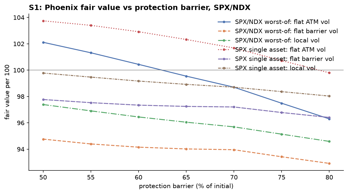
+
simulated book in its own units. The conversions:
|
|
10
|
+
|
|
11
|
+
half_spread_bps = cal["half_spread_bps"] already relative, in basis points
|
|
12
|
+
vol per bar = cal["mid_vol_per_sqrt_sec"] * sqrt(bar_seconds) diffusive scaling in time
|
|
13
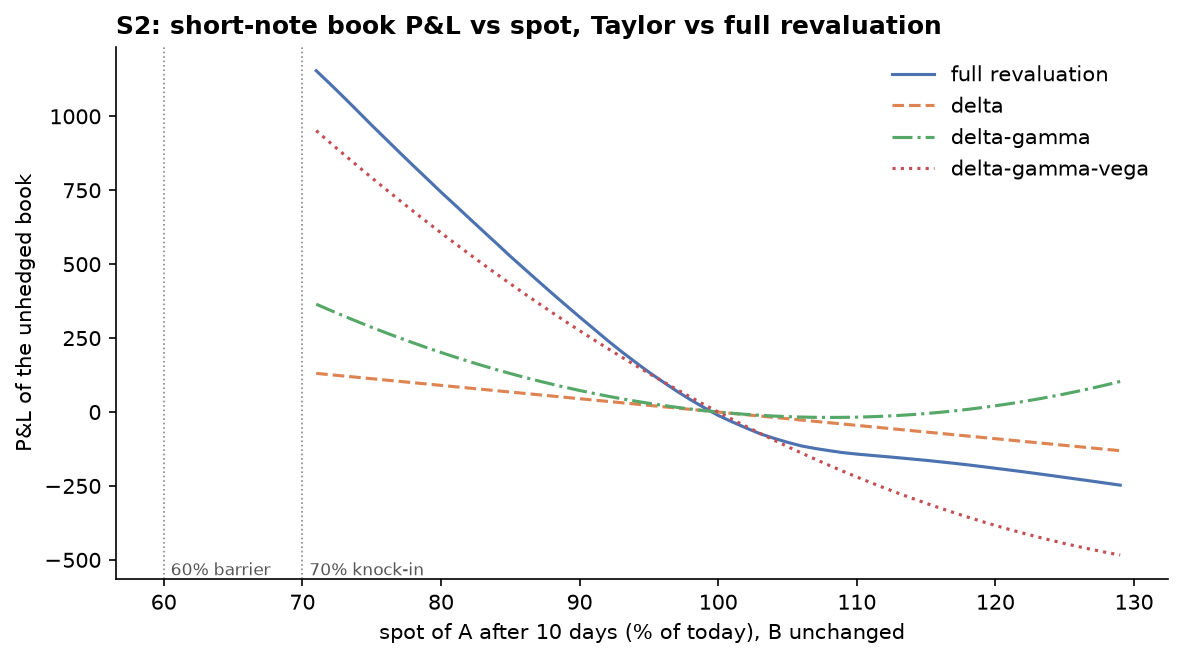
|
+
ADV per bar = cal["volume_per_sec"] * cal["mid_price"] * bar_seconds units/s -> quote ccy
|
|
14
|
+
Y matched to the measured OFI impact at a reference order size q_ref:
|
|
15
|
+
beta * q_ref / mid = Y * sigma_b * sqrt(q_ref / V_b)
|
|
16
|
+
beta: price change per unit of net order flow over one OFI bucket of b seconds
|
|
17
|
+
(Cont, Kukanov & Stoikov 2014); sigma_b, V_b: vol and volume over that bucket;
|
|
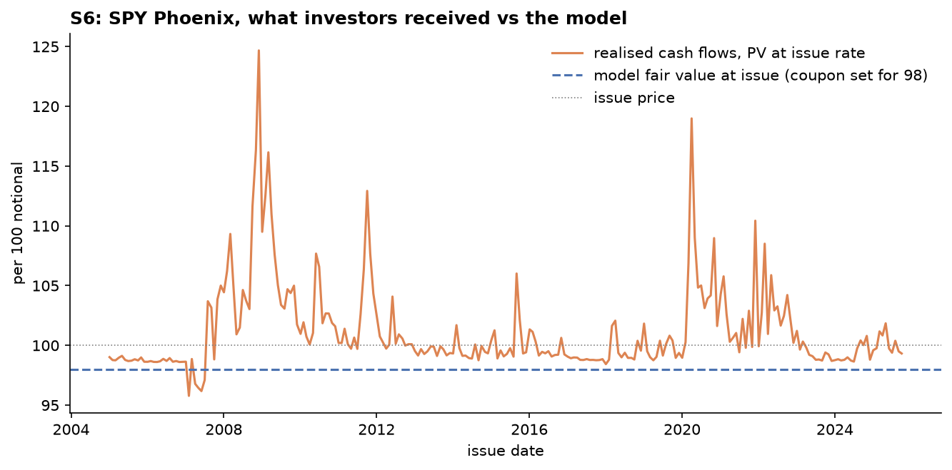
18
|
+
q_ref: the mean top-of-book depth, an order that just clears the best level.
|
|
19
|
+
|
|
20
|
+
The Y calibration is a modelling choice: OFI's impact is linear in flow and measured over seconds,
|
|
21
|
+
the square-root law is concave in size and meant for orders worked over a day. Matching them at one
|
|
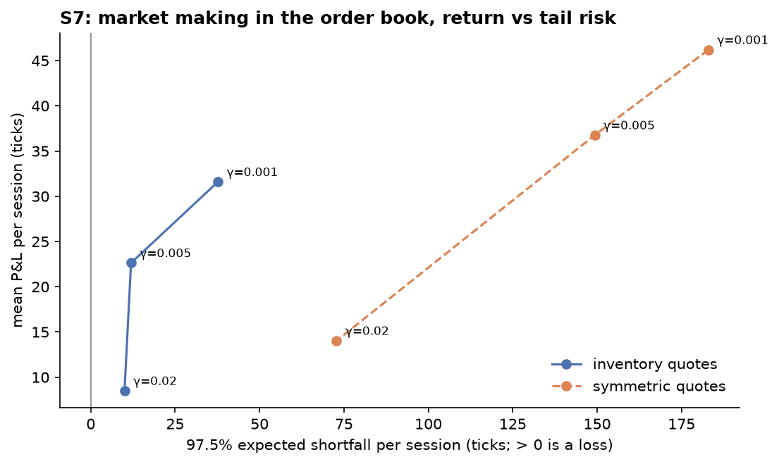
22
|
+
size gives the right order of magnitude, not a precise coefficient; S4 reports results for a range.
|
|
23
|
+
Passing impact_coef (e.g. the textbook Y = 1) overrides the calibration.
|
|
24
|
+
|
|
25
|
+
Fees. An order book shows the spread and the impact, not the venue's fee schedule, which is usually
|
|
26
|
+
the largest cost of trading a liquid crypto pair: Binance's published base spot taker fee is 0.10%
|
|
27
|
+
(10 bp) per trade, against a BTCUSDT half-spread under 0.001 bp. fee_bps is charged per unit traded,
|
|
28
|
+
like the half-spread, so it is added to SpreadImpactCost's linear term.
|
|
29
|
+
Clock: calibrate_costs uses the frames' timestamps (lobkit.load_recording puts quotes and trades on
|
|
30
|
+
the local receive clock), so per-second rates are wall-clock rates.
|
|
31
|
+
"""
|
|
32
|
+
|
|
33
|
+
from __future__ import annotations
|
|
34
|
+
|
|
35
|
+
from collections.abc import Mapping
|
|
36
|
+
|
|
37
|
+
import numpy as np
|
|
38
|
+
import pandas as pd
|
|
39
|
+
from btlab import SpreadImpactCost
|
|
40
|
+
|
|
41
|
+
SECONDS_PER_DAY_24H = 86_400.0 # crypto trades around the clock
|
|
42
|
+
|
|
43
|
+
|
|
44
|
+
def impact_coefficient(cal: Mapping, ofi_bucket_seconds: float = 10.0) -> float:
|
|
45
|
+
"""Square-root-law Y implied by the OFI impact slope at an order of the mean top-of-book size."""
|
|
46
|
+
q_ref = cal["mean_depth"]
|
|
47
|
+
linear = cal["ofi_impact_beta"] * q_ref / cal["mid_price"] # relative move for q_ref
|
|
48
|
+
sigma_b = cal["mid_vol_per_sqrt_sec"] * np.sqrt(ofi_bucket_seconds)
|
|
49
|
+
volume_b = cal["volume_per_sec"] * ofi_bucket_seconds
|
|
50
|
+
return float(linear / (sigma_b * np.sqrt(q_ref / volume_b)))
|
|
51
|
+
|
|
52
|
+
|
|
53
|
+
def bar_inputs(cal: Mapping, bar_seconds: float) -> dict:
|
|
54
|
+
"""Vol per bar and traded value (ADV) per bar, in the units SpreadImpactCost expects."""
|
|
55
|
+
return {"vol": cal["mid_vol_per_sqrt_sec"] * np.sqrt(bar_seconds),
|
|
56
|
+
"adv": cal["volume_per_sec"] * cal["mid_price"] * bar_seconds}
|
|
57
|
+
|
|
58
|
+
|
|
59
|
+
def cost_model_from_book(cal: Mapping | Mapping[str, Mapping], bar_seconds: float, capital: float,
|
|
60
|
+
impact_coef: float | None = None, ofi_bucket_seconds: float = 10.0,
|
|
61
|
+
fee_bps: float = 0.0) -> SpreadImpactCost:
|
|
62
|
+
"""SpreadImpactCost from one calibrate_costs dict, or from {asset: dict} for per-asset costs.
|
|
63
|
+
|
|
64
|
+
With several assets, half-spread and Y are taken per asset and averaged for Y (SpreadImpactCost has one
|
|
65
|
+
coefficient); vol and ADV stay per asset. impact_coef overrides the calibrated Y; fee_bps (exchange fee per
|
|
66
|
+
unit traded) is added to the half-spread.
|
|
67
|
+
"""
|
|
68
|
+
per_asset = all(isinstance(v, Mapping) for v in cal.values())
|
|
69
|
+
cals = dict(cal) if per_asset else {"_": cal}
|
|
70
|
+
ys = [impact_coefficient(c, ofi_bucket_seconds) for c in cals.values()]
|
|
71
|
+
y = float(np.mean(ys)) if impact_coef is None else impact_coef
|
|
72
|
+
if not per_asset:
|
|
73
|
+
inp = bar_inputs(cal, bar_seconds)
|
|
74
|
+
return SpreadImpactCost(cal["half_spread_bps"] + fee_bps, y, inp["adv"], inp["vol"], capital)
|
|
75
|
+
inputs = {a: bar_inputs(c, bar_seconds) for a, c in cals.items()}
|
|
76
|
+
spreads = [c["half_spread_bps"] for c in cals.values()]
|
|
77
|
+
# ponytail: one half-spread for all assets (SpreadImpactCost takes a scalar); the max is the cautious
|
|
78
|
+
# choice. Make half_spread_bps accept a per-asset Series in btlab if spreads differ a lot.
|
|
79
|
+
return SpreadImpactCost(max(spreads) + fee_bps, y, pd.Series({a: v["adv"] for a, v in inputs.items()}),
|
|
80
|
+
pd.Series({a: v["vol"] for a, v in inputs.items()}), capital)
|
|
@@ -0,0 +1,169 @@
|
|
|
1
|
+
"""sppricer notes as risklab positions (Link B).
|
|
2
|
+
|
|
3
|
+
risklab values a position by asking value(scenario) for a batch of scenarios (spot multipliers per
|
|
4
|
+
underlying, vol shift, skew shift, elapsed time). StructuredNotePosition answers by repricing the note
|
|
5
|
+
with sppricer's Monte Carlo; GridNotePosition answers from a precomputed price grid, which is what makes
|
|
6
|
+
thousands of VaR scenarios affordable.
|
|
7
|
+
|
|
8
|
+
Common random numbers. Every repricing uses the same seed and the same number and order of draws, so
|
|
9
|
+
the difference between two scenarios reflects the shock, not Monte Carlo noise. A scenario changes
|
|
10
|
+
only inputs (spots, vols, the schedule's distance from today), never the shape of the draw.
|
|
11
|
+
|
|
12
|
+
Elapsed time. Moving a live note forward changes its schedule and, once an observation passes, its
|
|
13
|
+
coupon memory and autocall state. This adapter does the conservative thing: elapsed time must be
|
|
14
|
+
shorter than the time to the first observation date, so the schedule only shifts closer and no state
|
|
15
|
+
changes. Longer horizons raise ValueError.
|
|
16
|
+
"""
|
|
17
|
+
|
|
18
|
+
from __future__ import annotations
|
|
19
|
+
|
|
20
|
+
from dataclasses import fields, replace
|
|
21
|
+
|
|
22
|
+
import numpy as np
|
|
23
|
+
from risklab import Scenario
|
|
24
|
+
from scipy.interpolate import RegularGridInterpolator
|
|
25
|
+
from sppricer import GBMModel, LocalVolModel, Market, price_mc
|
|
26
|
+
|
|
27
|
+
from quantstack.adapters.surface import SurfaceLocalVol
|
|
28
|
+
|
|
29
|
+
_SCHEDULE_FIELDS = ("observation_times", "coupon_times", "maturity")
|
|
30
|
+
SPOT_GRID = tuple(np.linspace(0.6, 1.4, 17))
|
|
31
|
+
VOL_GRID = tuple(np.linspace(-0.10, 0.15, 11)) # 2.5 vol-point steps: note prices are convex in vol
|
|
32
|
+
|
|
33
|
+
|
|
34
|
+
def shift_schedule(product, elapsed: float):
|
|
35
|
+
"""The same product seen `elapsed` years later; every date must still be in the future."""
|
|
36
|
+
if elapsed == 0:
|
|
37
|
+
return product
|
|
38
|
+
changes = {}
|
|
39
|
+
for f in fields(product):
|
|
40
|
+
if f.name in _SCHEDULE_FIELDS:
|
|
41
|
+
t = np.atleast_1d(np.asarray(getattr(product, f.name), dtype=float))
|
|
42
|
+
if elapsed >= t[0]:
|
|
43
|
+
raise ValueError(f"elapsed {elapsed:.4f}y reaches the first date {t[0]:.4f}y of {f.name}; "
|
|
44
|
+
"observation state (memory, autocall) is not modelled, so shorten the horizon")
|
|
45
|
+
shifted = t - elapsed
|
|
46
|
+
changes[f.name] = float(shifted[0]) if f.name == "maturity" else tuple(shifted)
|
|
47
|
+
return replace(product, **changes)
|
|
48
|
+
|
|
49
|
+
|
|
50
|
+
class _PayOn:
|
|
51
|
+
"""A 'market' whose discount factor is 1 on one date and 0 elsewhere, to read off a single cash flow."""
|
|
52
|
+
|
|
53
|
+
def __init__(self, t: float):
|
|
54
|
+
self.t = t
|
|
55
|
+
|
|
56
|
+
def discount(self, t):
|
|
57
|
+
return float(np.isclose(t, self.t))
|
|
58
|
+
|
|
59
|
+
|
|
60
|
+
def realised_cashflows(product, levels) -> np.ndarray:
|
|
61
|
+
"""Cash flow the note pays on each observation date if the underlyings print `levels` (n_dates x n_assets).
|
|
62
|
+
|
|
63
|
+
Runs the product's own payoff on the one realised path, so coupons, memory and autocall follow exactly
|
|
64
|
+
the rules used for pricing. Only for European barrier monitoring: a knock-in watched between dates
|
|
65
|
+
needs the whole path, not the observation levels.
|
|
66
|
+
"""
|
|
67
|
+
if getattr(product, "barrier_monitoring", "european") != "european":
|
|
68
|
+
raise ValueError("realised_cashflows needs barrier_monitoring='european'")
|
|
69
|
+
path = np.asarray(levels, dtype=float).reshape(1, len(product.simulation_times), -1)
|
|
70
|
+
return np.array([product.discounted_payoff(path, _PayOn(t))[0] for t in product.simulation_times])
|
|
71
|
+
|
|
72
|
+
|
|
73
|
+
class StructuredNotePosition:
|
|
74
|
+
"""`quantity` units of an sppricer product, revalued by Monte Carlo in each scenario.
|
|
75
|
+
|
|
76
|
+
Flat-vol mode (surfaces=None): GBM on `market`; vol_shift adds to each underlying's vol and
|
|
77
|
+
skew_shift is not available (a flat vol has no skew). Local-vol mode: `surfaces` (volsurface,
|
|
78
|
+
one per underlying, matching market.curves) drive sppricer's LocalVolModel; vol_shift and
|
|
79
|
+
skew_shift reshape them with surface.shifted, which rejects shifts that create arbitrage.
|
|
80
|
+
Under local vol a spot shock is sticky-strike: the surface stays put in absolute strike.
|
|
81
|
+
Prices are per the product's notional; value = quantity * price.
|
|
82
|
+
"""
|
|
83
|
+
|
|
84
|
+
def __init__(self, product, market: Market, quantity: float = 1.0, n_paths: int = 20_000, seed: int = 7,
|
|
85
|
+
surfaces=None, dt: float = 1 / 252):
|
|
86
|
+
self.product, self.market, self.quantity = product, market, quantity
|
|
87
|
+
self.n_paths, self.seed, self.surfaces, self.dt = n_paths, seed, surfaces, dt
|
|
88
|
+
|
|
89
|
+
def price(self, spot_mult, vol_shift: float = 0.0, skew_shift: float = 0.0, elapsed: float = 0.0):
|
|
90
|
+
"""(price, standard error) in one market state; spot_mult has one entry per underlying."""
|
|
91
|
+
m = self.market
|
|
92
|
+
for i, (u, x) in enumerate(zip(m.underlyings, np.broadcast_to(spot_mult, (m.n_assets,)), strict=True)):
|
|
93
|
+
m = m.with_spot(i, u.spot * float(x))
|
|
94
|
+
if self.surfaces is None and vol_shift:
|
|
95
|
+
m = m.with_vol(i, max(u.vol + vol_shift, 1e-4))
|
|
96
|
+
if self.surfaces is None:
|
|
97
|
+
if skew_shift:
|
|
98
|
+
raise ValueError("skew_shift needs local-vol mode (surfaces)")
|
|
99
|
+
model = GBMModel()
|
|
100
|
+
else:
|
|
101
|
+
surfs = self.surfaces if not (vol_shift or skew_shift) else \
|
|
102
|
+
[s.shifted(vol_shift, skew_shift) for s in self.surfaces]
|
|
103
|
+
model = LocalVolModel([SurfaceLocalVol(s) for s in surfs], dt=self.dt)
|
|
104
|
+
res = price_mc(shift_schedule(self.product, elapsed), m, self.n_paths, seed=self.seed, model=model)
|
|
105
|
+
return res.price, res.std_error
|
|
106
|
+
|
|
107
|
+
def value(self, scenario: Scenario) -> np.ndarray:
|
|
108
|
+
n = len(scenario)
|
|
109
|
+
mults = np.column_stack([scenario.spot(i) * np.ones(n) for i in range(self.market.n_assets)])
|
|
110
|
+
vs = np.broadcast_to(scenario.vol_shift, (n,))
|
|
111
|
+
ks = np.broadcast_to(scenario.skew_shift, (n,))
|
|
112
|
+
return self.quantity * np.array([self.price(mults[j], vs[j], ks[j], scenario.elapsed)[0]
|
|
113
|
+
for j in range(n)])
|
|
114
|
+
|
|
115
|
+
|
|
116
|
+
class GridNotePosition:
|
|
117
|
+
"""A StructuredNotePosition priced from a grid over (spot multiplier per underlying, vol shift).
|
|
118
|
+
|
|
119
|
+
The grid is computed at one horizon `elapsed` (the VaR horizon) and interpolated linearly, which is
|
|
120
|
+
monotone and does not overshoot near barriers. value() of the unshocked, elapsed=0 scenario (the
|
|
121
|
+
base risklab subtracts) is repriced directly, so P&L still includes time decay.
|
|
122
|
+
"""
|
|
123
|
+
|
|
124
|
+
def __init__(self, position: StructuredNotePosition, elapsed: float,
|
|
125
|
+
spot_mults=SPOT_GRID, vol_shifts=VOL_GRID):
|
|
126
|
+
# ponytail: linear interpolation on a fixed grid; refine near the barrier or go cubic if validate()
|
|
127
|
+
# shows errors above ~2 SE where the book's tail scenarios land.
|
|
128
|
+
self.position, self.elapsed = position, elapsed
|
|
129
|
+
self.spot_mults, self.vol_shifts = np.asarray(spot_mults, float), np.asarray(vol_shifts, float)
|
|
130
|
+
n = position.market.n_assets
|
|
131
|
+
axes = [self.spot_mults] * n + [self.vol_shifts]
|
|
132
|
+
prices = np.empty([len(a) for a in axes])
|
|
133
|
+
for idx in np.ndindex(*prices.shape):
|
|
134
|
+
prices[idx] = position.price([axes[a][i] for a, i in enumerate(idx[:n])], self.vol_shifts[idx[n]],
|
|
135
|
+
elapsed=elapsed)[0]
|
|
136
|
+
self.grid = RegularGridInterpolator(axes, prices, bounds_error=False, fill_value=None)
|
|
137
|
+
self.base = position.price(np.ones(n))[0]
|
|
138
|
+
|
|
139
|
+
def _points(self, scenario: Scenario) -> np.ndarray:
|
|
140
|
+
n_assets, n = self.position.market.n_assets, len(scenario)
|
|
141
|
+
cols = [scenario.spot(i) * np.ones(n) for i in range(n_assets)]
|
|
142
|
+
return np.column_stack(cols + [np.broadcast_to(scenario.vol_shift, (n,))])
|
|
143
|
+
|
|
144
|
+
def value(self, scenario: Scenario) -> np.ndarray:
|
|
145
|
+
if np.any(np.asarray(scenario.skew_shift) != 0):
|
|
146
|
+
raise ValueError("the price grid has no skew dimension")
|
|
147
|
+
pts = self._points(scenario)
|
|
148
|
+
if scenario.elapsed == 0 and np.allclose(pts[:, :-1], 1.0) and np.allclose(pts[:, -1], 0.0):
|
|
149
|
+
return self.position.quantity * np.full(len(pts), self.base)
|
|
150
|
+
if not np.isclose(scenario.elapsed, self.elapsed):
|
|
151
|
+
raise ValueError(f"grid built for elapsed={self.elapsed}, scenario has {scenario.elapsed}")
|
|
152
|
+
lo, hi = self.spot_mults[[0, -1]]
|
|
153
|
+
if np.any((pts[:, :-1] < lo) | (pts[:, :-1] > hi)):
|
|
154
|
+
raise ValueError(f"scenario spot multipliers leave the grid [{lo}, {hi}]")
|
|
155
|
+
return self.position.quantity * self.grid(pts)
|
|
156
|
+
|
|
157
|
+
def validate(self, n_points: int = 25, seed: int = 0) -> dict:
|
|
158
|
+
"""Grid vs direct Monte Carlo at random in-grid points: max |error| in price and in standard errors."""
|
|
159
|
+
rng = np.random.default_rng(seed)
|
|
160
|
+
n_assets = self.position.market.n_assets
|
|
161
|
+
lo, hi = self.spot_mults[[0, -1]]
|
|
162
|
+
pts = np.column_stack([rng.uniform(lo + 0.1, hi - 0.1, (n_points, n_assets)),
|
|
163
|
+
rng.uniform(self.vol_shifts[0], self.vol_shifts[-1], n_points)])
|
|
164
|
+
direct = np.array([self.position.price(p[:-1], p[-1], elapsed=self.elapsed) for p in pts])
|
|
165
|
+
err = self.grid(pts) - direct[:, 0]
|
|
166
|
+
noisy = direct[:, 1] > 1e-6 # deep in or out of the money a payoff can be riskless: SE ~ 0
|
|
167
|
+
in_se = np.abs(err[noisy] / direct[noisy, 1]).max() if noisy.any() else 0.0
|
|
168
|
+
return {"max_abs_error": float(np.abs(err).max()), "max_error_in_se": float(in_se),
|
|
169
|
+
"mean_abs_error": float(np.abs(err).mean()), "points": pts, "errors": err}
|
|
@@ -0,0 +1,56 @@
|
|
|
1
|
+
"""volsurface surfaces as sppricer local-vol sources (Link A).
|
|
2
|
+
|
|
3
|
+
Units. sppricer simulates absolute spot levels S_t in years t and asks a source
|
|
4
|
+
for local_vol(K, T) at K = S_t, T = t. volsurface surfaces take the same absolute
|
|
5
|
+
K and T and convert internally to log-moneyness k = ln(K / F(T)) on their own
|
|
6
|
+
forward curve F, the curve implied from the chain by put-call parity. So no
|
|
7
|
+
rescaling is needed, provided the simulation starts from the curve's spot and
|
|
8
|
+
drifts along the same curve. local_vol_setup builds the Market that way.
|
|
9
|
+
|
|
10
|
+
Safety. Paths reach strikes far outside the quoted range, where Dupire's formula
|
|
11
|
+
divides by numbers near zero. The adapter evaluates local vol with volsurface's
|
|
12
|
+
safe path: flat in k beyond the fitted range, NaN (arbitrage) replaced by implied
|
|
13
|
+
vol, clipped to [floor, cap]; surface.n_clamped / n_local_vol report how often.
|
|
14
|
+
"""
|
|
15
|
+
|
|
16
|
+
from __future__ import annotations
|
|
17
|
+
|
|
18
|
+
import numpy as np
|
|
19
|
+
from sppricer import LocalVolModel, Market, Underlying
|
|
20
|
+
from volsurface import VolSurface
|
|
21
|
+
|
|
22
|
+
|
|
23
|
+
class SurfaceLocalVol:
|
|
24
|
+
"""A volsurface surface seen through sppricer's LocalVolSource protocol."""
|
|
25
|
+
|
|
26
|
+
def __init__(self, surface: VolSurface, floor: float = 0.01, cap: float = 3.0):
|
|
27
|
+
self.surface, self.floor, self.cap = surface, floor, cap
|
|
28
|
+
|
|
29
|
+
@property
|
|
30
|
+
def curve(self):
|
|
31
|
+
return self.surface.curve
|
|
32
|
+
|
|
33
|
+
def local_vol(self, K, T):
|
|
34
|
+
return self.surface.local_vol(K, T, floor=self.floor, cap=self.cap, extrapolate="flat")
|
|
35
|
+
|
|
36
|
+
@property
|
|
37
|
+
def clamped_share(self) -> float:
|
|
38
|
+
s = self.surface
|
|
39
|
+
return s.n_clamped / s.n_local_vol if s.n_local_vol else 0.0
|
|
40
|
+
|
|
41
|
+
|
|
42
|
+
def local_vol_setup(surfaces: list[VolSurface], correlation=None, dt: float = 1 / 252,
|
|
43
|
+
names: list[str] | None = None, flat_vols=None) -> tuple[Market, LocalVolModel]:
|
|
44
|
+
"""(Market, LocalVolModel) whose spots and discounting come from the surfaces' own curves.
|
|
45
|
+
|
|
46
|
+
Spot of asset i = surfaces[i].curve.spot; each asset's forward curve is its
|
|
47
|
+
surface's curve (Market.curves), and discounting uses the first surface's
|
|
48
|
+
curve. flat_vols, one per asset, sets the Underlying vols used by GBM on the
|
|
49
|
+
same curves: the flat-vol benchmark.
|
|
50
|
+
"""
|
|
51
|
+
names = names or [f"S{i}" for i in range(len(surfaces))]
|
|
52
|
+
vols = flat_vols if flat_vols is not None else [0.2] * len(surfaces)
|
|
53
|
+
market = Market(tuple(Underlying(n, s.curve.spot, v) for n, s, v in zip(names, surfaces, vols, strict=True)),
|
|
54
|
+
rate=0.0, correlation=None if correlation is None else np.asarray(correlation, dtype=float),
|
|
55
|
+
curves=tuple(s.curve for s in surfaces), discount_curve=surfaces[0].curve)
|
|
56
|
+
return market, LocalVolModel([SurfaceLocalVol(s) for s in surfaces], dt=dt)
|
|
@@ -0,0 +1,321 @@
|
|
|
1
|
+
Metadata-Version: 2.4
|
|
2
|
+
Name: quantstack-lab
|
|
3
|
+
Version: 0.1.0
|
|
4
|
+
Summary: A connected quantitative finance research stack: structured product pricing, volatility surfaces, honest backtesting, market microstructure and risk, linked into end-to-end studies.
|
|
5
|
+
License-Expression: MIT
|
|
6
|
+
Project-URL: Repository, https://github.com/hossainyousuf751/quant-stack
|
|
7
|
+
Requires-Python: >=3.10
|
|
8
|
+
Description-Content-Type: text/markdown
|
|
9
|
+
License-File: LICENSE
|
|
10
|
+
Requires-Dist: sppricer<0.3,>=0.2.1
|
|
11
|
+
Requires-Dist: volsurface-lab<0.3,>=0.2.1
|
|
12
|
+
Requires-Dist: btlab<0.5,>=0.4.0
|
|
13
|
+
Requires-Dist: lobkit<0.4,>=0.3.0
|
|
14
|
+
Requires-Dist: marketrisk-lab<0.5,>=0.4.1
|
|
15
|
+
Requires-Dist: numpy>=1.24
|
|
16
|
+
Requires-Dist: scipy>=1.10
|
|
17
|
+
Requires-Dist: pandas>=2.0
|
|
18
|
+
Provides-Extra: dev
|
|
19
|
+
Requires-Dist: pytest>=7; extra == "dev"
|
|
20
|
+
Requires-Dist: matplotlib>=3.7; extra == "dev"
|
|
21
|
+
Dynamic: license-file
|
|
22
|
+
|
|
23
|
+
# quant-stack
|
|
24
|
+
|
|
25
|
+
> A connected quantitative finance research stack: structured product pricing, volatility
|
|
26
|
+
> surfaces, honest backtesting, market microstructure and risk, linked into end-to-end studies.
|
|
27
|
+
|
|
28
|
+
quant-stack holds five independent libraries as git submodules, pinned to tagged releases. It
|
|
29
|
+
connects them through small adapters and runs cross-project studies on top. No library imports
|
|
30
|
+
another, and none imports quant-stack. Each still installs, tests and releases on its own.
|
|
31
|
+
|
|
32
|
+
| Project | `pip install` (import) | What it does |
|
|
33
|
+
|---|---|---|
|
|
34
|
+
| [sp-pricer](https://github.com/hossainyousuf751/sp-pricer) | `sppricer` | Monte Carlo pricing of Phoenix autocallables and reverse convertibles, Greeks, barrier monitoring; Dupire local vol and term structure from v0.2 |
|
|
35
|
+
| [volsurface](https://github.com/hossainyousuf751/volsurface) | `volsurface-lab` (`volsurface`) | Arbitrage-free implied vol surfaces (SVI, SSVI, eSSVI, arbitrage-free SVI) from raw quotes, Dupire local vol, scenario shifts |
|
|
36
|
+
| [backtest-lab](https://github.com/hossainyousuf751/backtest-lab) | `btlab` | Backtesting with look-ahead tests, Deflated Sharpe, PBO, walk-forward, pluggable cost models, covariance strategies |
|
|
37
|
+
| [microstructure-lab](https://github.com/hossainyousuf751/microstructure-lab) | `lobkit` | Order-book reconstruction, order-flow imbalance, micro-price, Avellaneda–Stoikov; cost calibration and bars |
|
|
38
|
+
| [risk-lab](https://github.com/hossainyousuf751/risk-lab) | `marketrisk-lab` (`risklab`) | VaR/ES models and backtests, DCC-GARCH, shrinkage, HRP; scenario full-revaluation VaR and stress tests |
|
|
39
|
+
|
|
40
|
+
## How the pieces connect
|
|
41
|
+
|
|
42
|
+
```mermaid
|
|
43
|
+
flowchart LR
|
|
44
|
+
VS[volsurface] -->|"local_vol(K, T), curve<br/>adapters/surface.py"| SP[sp-pricer]
|
|
45
|
+
SP -->|"value(scenario)<br/>adapters/notes.py"| RL[risk-lab]
|
|
46
|
+
VS -->|"shifted surfaces, vol_fn"| RL
|
|
47
|
+
RL -->|"estimators and allocators<br/>(plain callables)"| BT[backtest-lab]
|
|
48
|
+
MS[microstructure-lab] -->|"calibrate_costs to SpreadImpactCost<br/>adapters/costs.py"| BT
|
|
49
|
+
subgraph quant-stack
|
|
50
|
+
A[adapters, studies S1-S7, integration tests]
|
|
51
|
+
end
|
|
52
|
+
```
|
|
53
|
+
|
|
54
|
+
Every arrow is a **protocol, not an import**. The library on the receiving end of an arrow defines a
|
|
55
|
+
small interface:
|
|
56
|
+
|
|
57
|
+
- sp-pricer's `LocalVolSource` is anything with `local_vol(K, T)` and a `curve`.
|
|
58
|
+
- risk-lab's `Position` is anything with `value(scenario)`.
|
|
59
|
+
- btlab's `CostModel` is anything with `cost(trade, date, context)`.
|
|
60
|
+
|
|
61
|
+
quant-stack wires real objects into those interfaces in [`src/quantstack/adapters/`](https://github.com/hossainyousuf751/quant-stack/tree/main/src/quantstack/adapters), and
|
|
62
|
+
nowhere else.
|
|
63
|
+
|
|
64
|
+
The libraries also duplicate a few small pieces on purpose instead of sharing a core package: three
|
|
65
|
+
Black-Scholes implementations and two yfinance loaders. [`tests/test_consistency.py`](https://github.com/hossainyousuf751/quant-stack/blob/main/tests/test_consistency.py)
|
|
66
|
+
asserts that the duplicates agree to 1e-12 on a grid of inputs and return the same data format.
|
|
67
|
+
|
|
68
|
+
## Studies
|
|
69
|
+
|
|
70
|
+
| Study | Question | Headline result |
|
|
71
|
+
|---|---|---|
|
|
72
|
+
| [S1](https://github.com/hossainyousuf751/quant-stack/blob/main/studies/s1_skew_autocallable.py) skew and the autocallable | What does pricing off the smile do to a Phoenix? | On the 2026-10-30 SPX/NDX close, local vol lowers the worst-of note from 100.44 to 96.44 per 100 (−4.00 ± 0.04 SE). The synthetic notes fall by 3.4 and 5.8 |
|
|
73
|
+
| [S2](https://github.com/hossainyousuf751/quant-stack/blob/main/studies/s2_note_book_risk.py) risk of a structured-note book | Where do linear VaR approximations break? | Delta-normal VaR of the delta-hedged book is 0, against 90 under full revaluation. Delta-gamma-vega overstates it at 152 |
|
|
74
|
+
| [S3](https://github.com/hossainyousuf751/quant-stack/blob/main/studies/s3_risk_portfolios_backtest.py) risk-based portfolios, honestly backtested | Do risk-lab's rankings survive costs, lag and selection? | Long-only minimum variance keeps the lowest true risk (9.5% vs 15.1% for 1/N) after lag and costs. Best of 24 configurations: Deflated Sharpe 0.94, walk-forward out-of-sample Sharpe 0.59. HRP's turnover barely falls with the window on synthetic data but falls 4× on real ETFs |
|
|
75
|
+
| [S4](https://github.com/hossainyousuf751/quant-stack/blob/main/studies/s4_costs_from_order_book.py) costs from the order book | Does a strong same-second order-flow relationship survive as a trade? | OFI (R² 0.59) loses after the spread alone. Queue imbalance survives spread, 1–5 s latency and the recorded book at small size, but covers at most 0.24 bp per unit traded, so any exchange taker fee kills it |
|
|
76
|
+
| [S5](https://github.com/hossainyousuf751/quant-stack/blob/main/studies/s5_skew_option_var.py) skew in option VaR | How much does the smile's behaviour under spot moves change option VaR? | Sticky moneyness more than doubles a short straddle's 1-day VaR against sticky strike (0.82 vs 0.38 synthetic, 0.84 vs 0.32 SPX) |
|
|
77
|
+
| [S6](https://github.com/hossainyousuf751/quant-stack/blob/main/studies/s6_autocallable_investors.py) how did autocallable investors do? | A SPY Phoenix issued monthly since 2005 at a model fair value of 98: what did investors actually receive? | Realised cash flows were worth 101.20 at the issue rate, +3.20 ± 0.72 (Newey-West) above the model. 94% autocalled, none lost capital, and the excess return over the 3-year rate was +1.1% ± 0.7% a year |
|
|
78
|
+
| [S7](https://github.com/hossainyousuf751/quant-stack/blob/main/studies/s7_market_maker_risk.py) market-maker inventory risk | How bad is a bad session for an Avellaneda–Stoikov quoter in the order book, and do standard VaR models know? | Symmetric quotes earn 46–65% more but carry 5–13× the 97.5% ES. Normal VaR fails 4 of 6 books (32–47 exceptions against 15), and RiskMetrics EWMA finds none on the inventory books because it assumes zero-mean P&L. Historical and FHS pass |
|
|
79
|
+
|
|
80
|
+
Each study prints its tables to [`docs/`](https://github.com/hossainyousuf751/quant-stack/tree/main/docs) (`s*_output.txt`, plus plots). All seeds are fixed.
|
|
81
|
+
|
|
82
|
+
### S1: skew and the autocallable
|
|
83
|
+
|
|
84
|
+
|
|
85
|
+
|
|
86
|
+
The note is sp-pricer's README note: 3 years, quarterly, a 2% memory coupon, autocall at 100% from
|
|
87
|
+
year 1, and 60% European protection. Every product here is short a down-and-in put, so the put skew
|
|
88
|
+
drives its value. Three models price the same note on the same forward curves and random numbers:
|
|
89
|
+
|
|
90
|
+
| SPX/NDX worst-of, ρ = 0.9 | Fair value | vs flat ATM | P(autocall at year 1) | P(knocked in) |
|
|
91
|
+
|---|---|---|---|---|
|
|
92
|
+
| flat ATM vol (18.2% / 23.8%) | 100.44 | | 47.0% | 7.7% |
|
|
93
|
+
| flat vol at the 60% strike | 94.15 | −6.29 ± 0.04 | 42.4% | 17.7% |
|
|
94
|
+
| Dupire local vol (arbitrage-free SVI) | **96.44** | **−4.00 ± 0.04** | 57.4% | 11.2% |
|
|
95
|
+
|
|
96
|
+
The local-vol pipeline is validated first, in [`tests/test_link_a.py`](https://github.com/hossainyousuf751/quant-stack/blob/main/tests/test_link_a.py). Monte
|
|
97
|
+
Carlo prices of 20 vanillas under sp-pricer's `LocalVolModel` imply back the volsurface surface's
|
|
98
|
+
own vols within 2.5 standard errors. Flat ATM vol misses the same targets by up to 940.
|
|
99
|
+
|
|
100
|
+
The S1 numbers also reproduce volsurface's earlier, independent simulator: 100.41, 96.14 and 96.42.
|
|
101
|
+
Halving or doubling the time step moves the worst-of note by no more than its standard error (96.23,
|
|
102
|
+
96.30 and 96.15, each ± 0.07).
|
|
103
|
+
|
|
104
|
+
### S2: risk of a structured-note book
|
|
105
|
+
|
|
106
|
+
|
|
107
|
+
|
|
108
|
+
A dealer is short four notes on two underlyings and may delta-hedge with shares. Each method gives a
|
|
109
|
+
10-day 99% VaR (lognormal scenarios, with implied vol falling 0.8 points per 1% rise in A):
|
|
110
|
+
|
|
111
|
+
| Book | Delta-normal | Delta-gamma-vega | Full revaluation (price grid) |
|
|
112
|
+
|---|---|---|---|
|
|
113
|
+
| unhedged | 89.9 | 222.4 | 154.4 |
|
|
114
|
+
| delta-hedged | **0.0** | 152.2 | **90.0** |
|
|
115
|
+
|
|
116
|
+
Full revaluation reprices every note in every scenario. To make 20,000 scenarios affordable, it
|
|
117
|
+
interpolates on a price grid validated against direct repricing at random points: the mean error is
|
|
118
|
+
0.02 per 100 and the largest is 2.2 Monte Carlo standard errors.
|
|
119
|
+
The same pattern holds under fat-tailed DCC-t scenarios.
|
|
120
|
+
|
|
121
|
+
### S5: skew in option VaR
|
|
122
|
+
|
|
123
|
+
risk-lab Study 3's books, priced off a fitted smile instead of one flat vol, with full revaluation only:
|
|
124
|
+
|
|
125
|
+
| 1-day 99% VaR | flat ATM | sticky strike | sticky moneyness |
|
|
126
|
+
|---|---|---|---|
|
|
127
|
+
| covered call | 1.97 | 2.05 | 1.92 |
|
|
128
|
+
| protective put | 1.86 | 1.83 | 2.04 |
|
|
129
|
+
| short ATM straddle | 0.38 | 0.38 | **0.82** |
|
|
130
|
+
|
|
131
|
+
(Synthetic SSVI surface; the SPX snapshot gives the same ordering.)
|
|
132
|
+
|
|
133
|
+
### S6: how did autocallable investors actually do?
|
|
134
|
+
|
|
135
|
+
|
|
136
|
+
|
|
137
|
+
A 3-year SPY Phoenix is issued on the first trading day of every month from 2005 to 2025: quarterly
|
|
138
|
+
observations, a memory coupon above 70%, autocall at 100% from year 1, and 60% European protection.
|
|
139
|
+
The coupon is set at issue, from that day's VIX and Treasury yields only, so that sp-pricer's fair value
|
|
140
|
+
is 98 (a 2-point margin). The realised SPY path, from btlab's loader, then gives each note's actual cash
|
|
141
|
+
flows, read off by the product's own payoff code.
|
|
142
|
+
|
|
143
|
+
| 250 notes, 2005-01 to 2025-10 | Value |
|
|
144
|
+
|---|---|
|
|
145
|
+
| coupon set at issue, per year | mean 3.23%, from −0.32% (2013) to 28.4% (Nov 2008) |
|
|
146
|
+
| model fair value at issue | 98.00 |
|
|
147
|
+
| realised cash flows, PV at the issue rate | **101.20** (+3.20 ± 0.72) |
|
|
148
|
+
| realised IRR minus the 3-year rate | +1.13% ± 0.69% a year |
|
|
149
|
+
| outcomes | 94% autocalled (83% at year 1), 6% repaid at par, 0 losses |
|
|
150
|
+
| VIX at issue vs realised vol over the note's life | 19.3% vs 17.0% |
|
|
151
|
+
|
|
152
|
+
VIX stands in for a 3-year ATM vol, with no skew or term structure. The note is on SPY total return with
|
|
153
|
+
zero dividend yield, and the rate carries no issuer funding spread. The 21 years of overlapping notes hold
|
|
154
|
+
only about seven independent 3-year windows.
|
|
155
|
+
|
|
156
|
+
### S7: market-maker inventory risk
|
|
157
|
+
|
|
158
|
+
|
|
159
|
+
|
|
160
|
+
microstructure-lab's Avellaneda–Stoikov quoter runs inside its order-book simulator for 2,500 independent
|
|
161
|
+
5-minute sessions per setting. It uses the paper's inputs calibrated on the book, as in that repo's Study 4.
|
|
162
|
+
risk-lab measures each P&L series and backtests its four VaR models over the last 1,500 sessions.
|
|
163
|
+
|
|
164
|
+
| Session P&L (ticks) | Mean | Skew | Excess kurtosis | P(loss) | 99% VaR | 97.5% ES | Mean / ES |
|
|
165
|
+
|---|---|---|---|---|---|---|---|
|
|
166
|
+
| γ = 0.001, inventory | 31.6 | −0.57 | 0.8 | 9.9% | 37.0 | 37.7 | 0.84 |
|
|
167
|
+
| γ = 0.001, symmetric | 46.2 | −1.29 | 6.3 | 16.7% | 169.0 | 182.9 | 0.25 |
|
|
168
|
+
| **γ = 0.005, inventory** | **22.6** | −0.25 | 0.6 | **4.3%** | **10.0** | **11.9** | **1.90** |
|
|
169
|
+
| γ = 0.005, symmetric | 36.8 | −1.03 | 4.9 | 17.8% | 143.0 | 149.3 | 0.25 |
|
|
170
|
+
| γ = 0.02, inventory | 8.5 | −0.27 | 0.5 | 10.1% | 10.5 | 10.0 | 0.85 |
|
|
171
|
+
| γ = 0.02, symmetric | 14.0 | −1.00 | 5.9 | 21.6% | 70.0 | 72.8 | 0.19 |
|
|
172
|
+
|
|
173
|
+
| 99% VaR backtest, 6 books | Kupiec passes (p > 0.05) | Exceptions (15 expected) | 97.5% ES (Z2) |
|
|
174
|
+
|---|---|---|---|
|
|
175
|
+
| historical, 500 sessions | 6 of 6 | 13–21 | passes everywhere |
|
|
176
|
+
| filtered historical (FHS), 1,000 | 5 of 6 | 11–24 | passes everywhere |
|
|
177
|
+
| normal, 500 | 2 of 6, both at p = 0.054 | 23–47 | rejected on 4 books (−0.96 to −1.35) |
|
|
178
|
+
| EWMA (RiskMetrics) | 3 of 6: symmetric books only | 0 on every inventory book | far too conservative on inventory books |
|
|
179
|
+
|
|
180
|
+
In the paper's own fill model, not one of 2,500 sessions loses money (the worst is +43), so a loss VaR
|
|
181
|
+
there is meaningless. Losses come from the order book's queue position and adverse selection.
|
|
182
|
+
|
|
183
|
+
## What was surprising, what went wrong, and how it was diagnosed
|
|
184
|
+
|
|
185
|
+
**S1: a "skew-aware" flat vol overshoots.** Pricing the note with flat vol taken at the barrier
|
|
186
|
+
strike sounds like a cheap way to respect the skew, so I expected it to land near local vol. It lands
|
|
187
|
+
well below it instead: −6.3 against −4.0 on SPX/NDX, and −8.1 against −5.8 on the synthetic worst-of.
|
|
188
|
+
The autocall probabilities show why. A barrier-strike vol applies put-wing volatility everywhere,
|
|
189
|
+
including near and above 100%, where local vol is low. So it understates the chance of an early
|
|
190
|
+
call at year 1 (42% vs 57%) and overstates the chance of ending knocked in (18% vs 11%). Local vol
|
|
191
|
+
is not "flat vol at the right strike"; it is a different vol in each region the path visits. The
|
|
192
|
+
local-vol pipeline was validated before any of this: Monte Carlo vanillas reprice the surface within
|
|
193
|
+
2.5 SE, and two independent simulators agree within error.
|
|
194
|
+
|
|
195
|
+
**S2: delta-gamma-vega was worse than delta-normal, in the other direction.** I expected the
|
|
196
|
+
second-order expansion to land between delta-normal and full revaluation. Instead it overstates the
|
|
197
|
+
unhedged book's VaR by 44% (222 vs 154). To find out why, I repriced each note under parallel vol
|
|
198
|
+
shifts. The notes' value is concave in vol: an 8-point fall in vol raises the single-asset Phoenix by
|
|
199
|
+
3.8 per 100, while vega × shift says 4.9. The scenarios move vol against spot (−0.8 points per 1%),
|
|
200
|
+
so the 10-day tail combines a rally with a large vol fall, exactly where linear vega overstates the
|
|
201
|
+
dealer's loss. Delta-normal misses the other way: it reports zero risk for the delta-hedged book,
|
|
202
|
+
which full revaluation puts at 90. Getting the full-revaluation number cheaply also took a second
|
|
203
|
+
attempt. The first price grid missed direct repricing by up to 5.5 SE. That pointed at the vol axis
|
|
204
|
+
rather than the spot axis, because tightening the spot spacing made no difference. Halving the vol
|
|
205
|
+
step brought the worst point to 2.2 SE, and the VaR itself moved by only 2%.
|
|
206
|
+
|
|
207
|
+
**S3: one finding confirmed, one refuted, one bug of my own.** On risk-lab's synthetic data, HRP's
|
|
208
|
+
turnover barely falls as the estimation window grows (4.4 to 3.3 times a year, while minimum variance
|
|
209
|
+
falls from 5.6 to 1.0), confirming risk-lab's result under a real backtest. On the 10 ETFs it falls
|
|
210
|
+
4×, from 3.6 to 0.9. The block covariance's equal within-block correlations make HRP's ordering flip
|
|
211
|
+
between near-ties, while stocks, bonds and commodities form stable clusters. FHS VaR, which passes
|
|
212
|
+
every backtest on synthetic data, takes 44–53 exceptions against 37 expected on the ETF portfolios.
|
|
213
|
+
A first run also reported "true" volatility well below realised volatility for every method. The
|
|
214
|
+
cause was in my study code: it averaged in the warm-up rebalances that hold nothing. 24 empty
|
|
215
|
+
rebalances out of 144 explained the gap exactly (12.6% vs 15.1% for 1/N).
|
|
216
|
+
|
|
217
|
+
**S4: the edge that should not have survived, and what finally killed it.** The expected lesson was
|
|
218
|
+
that a strong same-second relationship (OFI explains 59% of BTC's one-second mid changes) does not
|
|
219
|
+
survive latency and spread. For OFI itself that holds: it trades about 2,000 times an hour, and the
|
|
220
|
+
spread alone costs more than its gross edge, so its net Sharpe is negative at every lag. Queue
|
|
221
|
+
imbalance did survive: positive net of spread and calibrated impact at lags of 1, 2 and 5 seconds,
|
|
222
|
+
right on 90% of the mid's moves. I treated that as a bug until each candidate was ruled out:
|
|
223
|
+
|
|
224
|
+
- The look-ahead check rebuilds features from quotes truncated at each cutoff, and it passes.
|
|
225
|
+
- The spread at the trades' execution bars equals the median spread, so the edge is not a wide
|
|
226
|
+
spread being ignored.
|
|
227
|
+
- Walking each trade through the recorded 10-level book at $100,000 cuts BTC's edge by a third but
|
|
228
|
+
leaves it positive. On the thinner ETH book the same size turns every variant negative; at $1,000
|
|
229
|
+
both survive.
|
|
230
|
+
|
|
231
|
+
What kills it is the cost an order book does not show: exchange fees. The signal's gross edge
|
|
232
|
+
covers at most about 0.24 bp per unit traded on BTC and on ETH, against Binance's
|
|
233
|
+
published base taker fee of 10 bp. At any taker fee, every variant loses. A queue-imbalance edge
|
|
234
|
+
belongs to whoever is paid to provide liquidity, not to whoever takes it. Two hours of data is one
|
|
235
|
+
sample, so this is an illustration of the method rather than a result to trade on.
|
|
236
|
+
|
|
237
|
+
**S6: investors beat the model, and the sample is why to be careful.** Priced at 98, the notes
|
|
238
|
+
delivered 101.20 on average. Only 2% of issues came in below 98, and the gap survives dropping the 2008,
|
|
239
|
+
2009 and 2020 vintages (+2.28 ± 0.38). The reason is in the outcomes: the fair value charges for a
|
|
240
|
+
3-year fall of more than 40%, and since 2005 the lowest SPY level at any 3-year maturity was 72%. VIX
|
|
241
|
+
also exceeded the volatility that followed for 65% of issues. Two results surprised me. First, for 13
|
|
242
|
+
issues between 2013 and 2016 the coupon that prices the note at 98 is negative: with VIX near 12 and
|
|
243
|
+
3-year rates under 1%, a note with no coupon is already worth more than 98. Real notes paid positive
|
|
244
|
+
coupons then because issuers fund above Treasuries and the note references the price index, which has
|
|
245
|
+
a lower forward; both are left out here and stated. Second, the first version used a fixed 8% coupon,
|
|
246
|
+
which put fair values as high as 112, terms no issuer would sell; setting the coupon at issue fixed that.
|
|
247
|
+
The study begins in 2005, as specified, so it leaves out 2000–2002, when SPY fell 48% peak to trough.
|
|
248
|
+
I first wrote here that a note issued in 2000 would very likely have lost capital, then checked the same
|
|
249
|
+
total-return series. It would not: the 2000 issues end at 60–85% of their initial level. The April 2000
|
|
250
|
+
note matures at 60.4%, just 0.4 points above the barrier. None of them autocalls, so investors get par
|
|
251
|
+
back after three years with most coupons missed. Seven independent windows cannot show that the model
|
|
252
|
+
overprices the crash; they show that a crash deep enough to breach 60% at a maturity date did not occur.
|
|
253
|
+
|
|
254
|
+
**S7: the model that failed for the opposite reason, and a library number that moved.** I expected
|
|
255
|
+
normal VaR to fail on the symmetric quoter, whose P&L has excess kurtosis near 6 and a fat left tail, and it
|
|
256
|
+
did, with 32–47 exceptions against 15. The surprise was RiskMetrics EWMA, which recorded zero exceptions on
|
|
257
|
+
every inventory book. It assumes zero-mean returns, but these books earn 1.2–1.7 standard deviations per
|
|
258
|
+
session on average. EWMA therefore reads the mean as volatility and sets VaR 2.6–5.7× too high (61 against 11
|
|
259
|
+
at γ = 0.005). Fed into a limit framework, that would cap the safest quoter hardest. Sessions are
|
|
260
|
+
independent by construction, so FHS has no clustering to exploit; it passes because its residuals are
|
|
261
|
+
empirical. Its one Kupiec rejection (p = 0.032) is in line with 24 tests at a 5% level.
|
|
262
|
+
|
|
263
|
+
Running 2,500 sessions instead of 200 also moved a number in microstructure-lab's README. Its γ = 0.005
|
|
264
|
+
inventory row shows a mean P&L of 19.4. The first 200 sessions here reproduce that exactly, but the full
|
|
265
|
+
2,500 average 22.6 ± 0.26, and five fresh blocks on unused seeds give 21.3–24.1. Seeds 0–199 were a
|
|
266
|
+
low draw, about 3.5 standard errors under the mean. Inventory control costs 32–40% of mean P&L rather than
|
|
267
|
+
the published 33–45%; the conclusion is unchanged. The library README is left as published until the
|
|
268
|
+
owner approves a change.
|
|
269
|
+
|
|
270
|
+
**Testing across versions.** The libraries promise numpy ≥ 1.24, pandas ≥ 2.0 and scipy ≥ 1.10. I
|
|
271
|
+
ran every suite in an environment with exactly those versions. Every test passed except my new
|
|
272
|
+
regression pins: optimiser-fitted values move by up to 1e-5 relative between scipy 1.10 and 1.17,
|
|
273
|
+
and one penalised SVI fit settles on a different optimum (0.1815 vs 0.1790, both printed as 0.18).
|
|
274
|
+
The pins now hold each figure to the precision the README actually prints.
|
|
275
|
+
|
|
276
|
+
## Install
|
|
277
|
+
|
|
278
|
+
```bash
|
|
279
|
+
pip install quantstack-lab # the adapters (import quantstack) and all five libraries from PyPI
|
|
280
|
+
```
|
|
281
|
+
|
|
282
|
+
`volsurface` and `risk-lab` are published as `volsurface-lab` and `marketrisk-lab`, because the names
|
|
283
|
+
`volsurface` and `risklab` belong to unrelated projects on PyPI; their import names are unchanged. The
|
|
284
|
+
studies, tests and plots are not part of the package. To run them, clone the repository as below.
|
|
285
|
+
|
|
286
|
+
## Reproduce
|
|
287
|
+
|
|
288
|
+
```bash
|
|
289
|
+
git clone --recurse-submodules https://github.com/hossainyousuf751/quant-stack.git
|
|
290
|
+
cd quant-stack
|
|
291
|
+
for p in sp-pricer volsurface backtest-lab microstructure-lab risk-lab; do pip install -e "projects/$p"; done
|
|
292
|
+
pip install -e ".[dev]"
|
|
293
|
+
pytest # consistency and integration tests, offline, about 1 minute
|
|
294
|
+
python studies/s1_skew_autocallable.py # each study writes docs/s*_output.txt-style tables and plots
|
|
295
|
+
```
|
|
296
|
+
|
|
297
|
+
What the studies need:
|
|
298
|
+
|
|
299
|
+
- **S1 and S5** use volsurface's saved CBOE snapshot (`projects/volsurface/data/`, git-ignored; create it with
|
|
300
|
+
`projects/volsurface/examples/snapshot.py`) for their real-data parts, and skip those parts without it.
|
|
301
|
+
- **S4** uses microstructure-lab's Binance recordings, likewise git-ignored and created with its recorder.
|
|
302
|
+
- **S7** is fully offline (simulated order book), about 7 minutes.
|
|
303
|
+
- **S3, S4 and S6** download Yahoo Finance prices on first run and cache them in `data/`. They skip those
|
|
304
|
+
parts when offline.
|
|
305
|
+
|
|
306
|
+
Each library's own tests still run without the others installed: `cd projects/<repo> && pytest`.
|
|
307
|
+
|
|
308
|
+
## Layout
|
|
309
|
+
|
|
310
|
+
```
|
|
311
|
+
quant-stack/
|
|
312
|
+
├── projects/ the five libraries (git submodules, tagged releases)
|
|
313
|
+
├── src/quantstack/
|
|
314
|
+
│ └── adapters/ surface.py (Link A), notes.py (Link B), costs.py (Link D)
|
|
315
|
+
├── studies/ S1-S7
|
|
316
|
+
├── tests/ consistency and integration tests
|
|
317
|
+
└── docs/ study outputs and plots; profile_README.md
|
|
318
|
+
```
|
|
319
|
+
|
|
320
|
+
Data is public or synthetic only: Yahoo Finance, CBOE delayed quotes, Binance public market data,
|
|
321
|
+
and simulators.
|
|
@@ -0,0 +1,10 @@
|
|
|
1
|
+
quantstack/__init__.py,sha256=PA1QRuW40bn1LjnVHVUV5G0w11e1EPWJyI3WbS9JerA,108
|
|
2
|
+
quantstack/adapters/__init__.py,sha256=eb1t39fV_Vo6NomuBZAmNHqN0HvBFdegfzR91euuqhM,77
|
|
3
|
+
quantstack/adapters/costs.py,sha256=TKg0qbA71OK5qjAfAoJSx4N9TsoIiHiWBu77CQ4w5Vw,4767
|
|
4
|
+
quantstack/adapters/notes.py,sha256=Q2Ygg6ZYIHUqxPyd_PaMHgDBdzgsKcpDeMGOpCwy-pY,9386
|
|
5
|
+
quantstack/adapters/surface.py,sha256=DIrPo-bV3CBBzgQODBKFm9Q6N7sVLy327DoaDg6xAGU,2714
|
|
6
|
+
quantstack_lab-0.1.0.dist-info/licenses/LICENSE,sha256=OAV_RTERHYKJrtHIxvr_VWUiM6k-1PKksx8ezi9wMmY,1079
|
|
7
|
+
quantstack_lab-0.1.0.dist-info/METADATA,sha256=Rsm50SfwANCAvKwKjk2fzo_6huCVhpOLe7hnt3mFJkQ,22491
|
|
8
|
+
quantstack_lab-0.1.0.dist-info/WHEEL,sha256=mOdXR9C3wMVov7cSY8PY-XCzo3SmmWCHvGQr5csJoao,91
|
|
9
|
+
quantstack_lab-0.1.0.dist-info/top_level.txt,sha256=plf1I8JuPOFml6zbDMp0A8_qLtg7ChacKDwmbipwe1U,11
|
|
10
|
+
quantstack_lab-0.1.0.dist-info/RECORD,,
|
|
@@ -0,0 +1,21 @@
|
|
|
1
|
+
MIT License
|
|
2
|
+
|
|
3
|
+
Copyright (c) 2026 Yousuf Hossain Shafeen
|
|
4
|
+
|
|
5
|
+
Permission is hereby granted, free of charge, to any person obtaining a copy
|
|
6
|
+
of this software and associated documentation files (the "Software"), to deal
|
|
7
|
+
in the Software without restriction, including without limitation the rights
|
|
8
|
+
to use, copy, modify, merge, publish, distribute, sublicense, and/or sell
|
|
9
|
+
copies of the Software, and to permit persons to whom the Software is
|
|
10
|
+
furnished to do so, subject to the following conditions:
|
|
11
|
+
|
|
12
|
+
The above copyright notice and this permission notice shall be included in all
|
|
13
|
+
copies or substantial portions of the Software.
|
|
14
|
+
|
|
15
|
+
THE SOFTWARE IS PROVIDED "AS IS", WITHOUT WARRANTY OF ANY KIND, EXPRESS OR
|
|
16
|
+
IMPLIED, INCLUDING BUT NOT LIMITED TO THE WARRANTIES OF MERCHANTABILITY,
|
|
17
|
+
FITNESS FOR A PARTICULAR PURPOSE AND NONINFRINGEMENT. IN NO EVENT SHALL THE
|
|
18
|
+
AUTHORS OR COPYRIGHT HOLDERS BE LIABLE FOR ANY CLAIM, DAMAGES OR OTHER
|
|
19
|
+
LIABILITY, WHETHER IN AN ACTION OF CONTRACT, TORT OR OTHERWISE, ARISING FROM,
|
|
20
|
+
OUT OF OR IN CONNECTION WITH THE SOFTWARE OR THE USE OR OTHER DEALINGS IN THE
|
|
21
|
+
SOFTWARE.
|
|
@@ -0,0 +1 @@
|
|
|
1
|
+
quantstack
|