pylocuszoom 1.2.0__py3-none-any.whl → 1.3.1__py3-none-any.whl

{pylocuszoom-1.2.0.dist-info → pylocuszoom-1.3.1.dist-info}/METADATA

@@ -1,6 +1,6 @@
 Metadata-Version: 2.4
 Name: pylocuszoom
-Version: 1.2.0
+Version: 1.3.1
 Summary: Publication-ready regional association plots with LD coloring, gene tracks, and recombination overlays
 Project-URL: Homepage, https://github.com/michael-denyer/pylocuszoom
 Project-URL: Documentation, https://github.com/michael-denyer/pylocuszoom#readme
@@ -72,20 +72,23 @@ Inspired by [LocusZoom](http://locuszoom.org/) and [locuszoomr](https://github.c
     - **SNP labels (matplotlib)**: Automatic labeling of top SNPs by p-value (RS IDs)
     - **Hover tooltips (Plotly and Bokeh)**: Detailed SNP data on hover
 
-![Example regional association plot with LD coloring, gene track, and recombination overlay](https://raw.githubusercontent.com/michael-denyer/pyLocusZoom/main/examples/regional_plot_with_recomb.png)
+![Example regional association plot with LD coloring, gene track, and recombination overlay](https://raw.githubusercontent.com/michael-denyer/pyLocusZoom/main/examples/matplotlib/regional_plot_with_recomb.png)
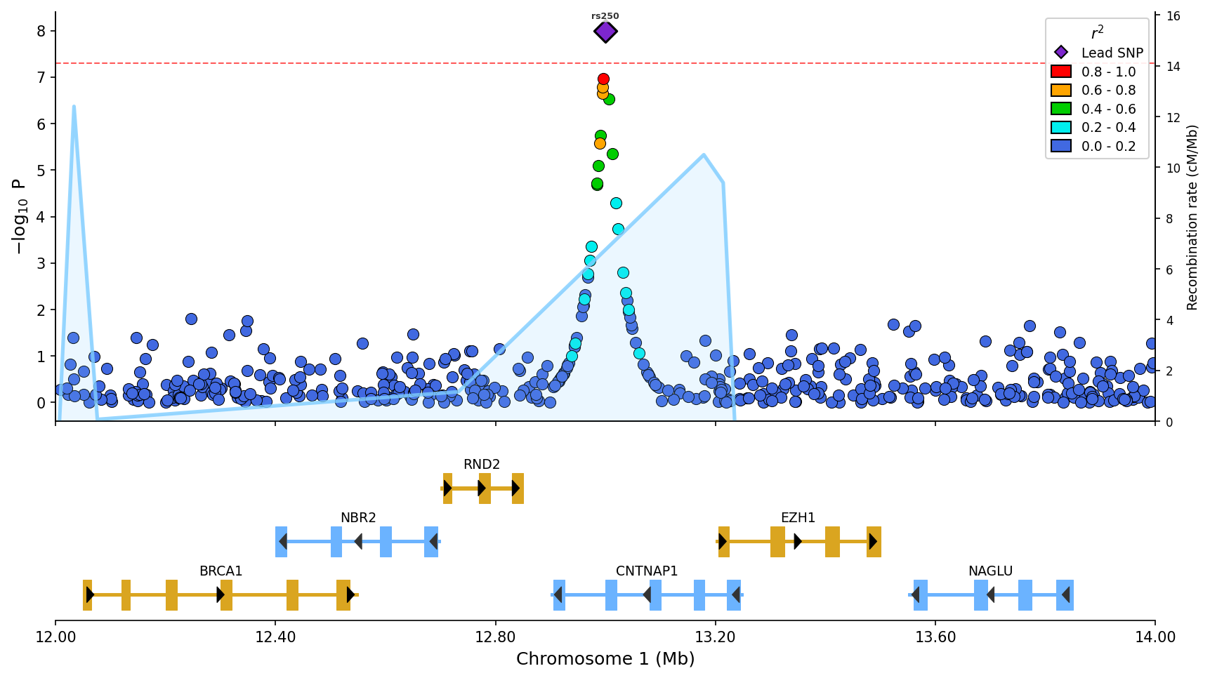
 *Regional association plot with LD coloring, gene/exon track, recombination rate overlay (blue line), and top SNP labels.*
 
 2. **Stacked plots**: Compare multiple GWAS/phenotypes vertically
-3. **Manhattan plots**: Genome-wide association visualization with chromosome coloring
-4. **QQ plots**: Quantile-quantile plots with confidence bands and genomic inflation factor
-5. **eQTL plot**: Expression QTL data aligned with association plots and gene tracks
-6. **Fine-mapping plots**: Visualize SuSiE credible sets with posterior inclusion probabilities
-7. **PheWAS plots**: Phenome-wide association study visualization across multiple phenotypes
-8. **Forest plots**: Meta-analysis effect size visualization with confidence intervals
-9. **Multiple backends**: matplotlib (publication-ready), plotly (interactive), bokeh (dashboard integration)
-10. **Pandas and PySpark support**: Works with both Pandas and PySpark DataFrames for large-scale genomics data
-11. **Convenience data file loaders**: Load and validate common GWAS, eQTL and fine-mapping file formats
-12. **Automatic gene annotations**: Fetch gene/exon data from Ensembl REST API with caching (human, mouse, rat, canine, feline, and any Ensembl species)
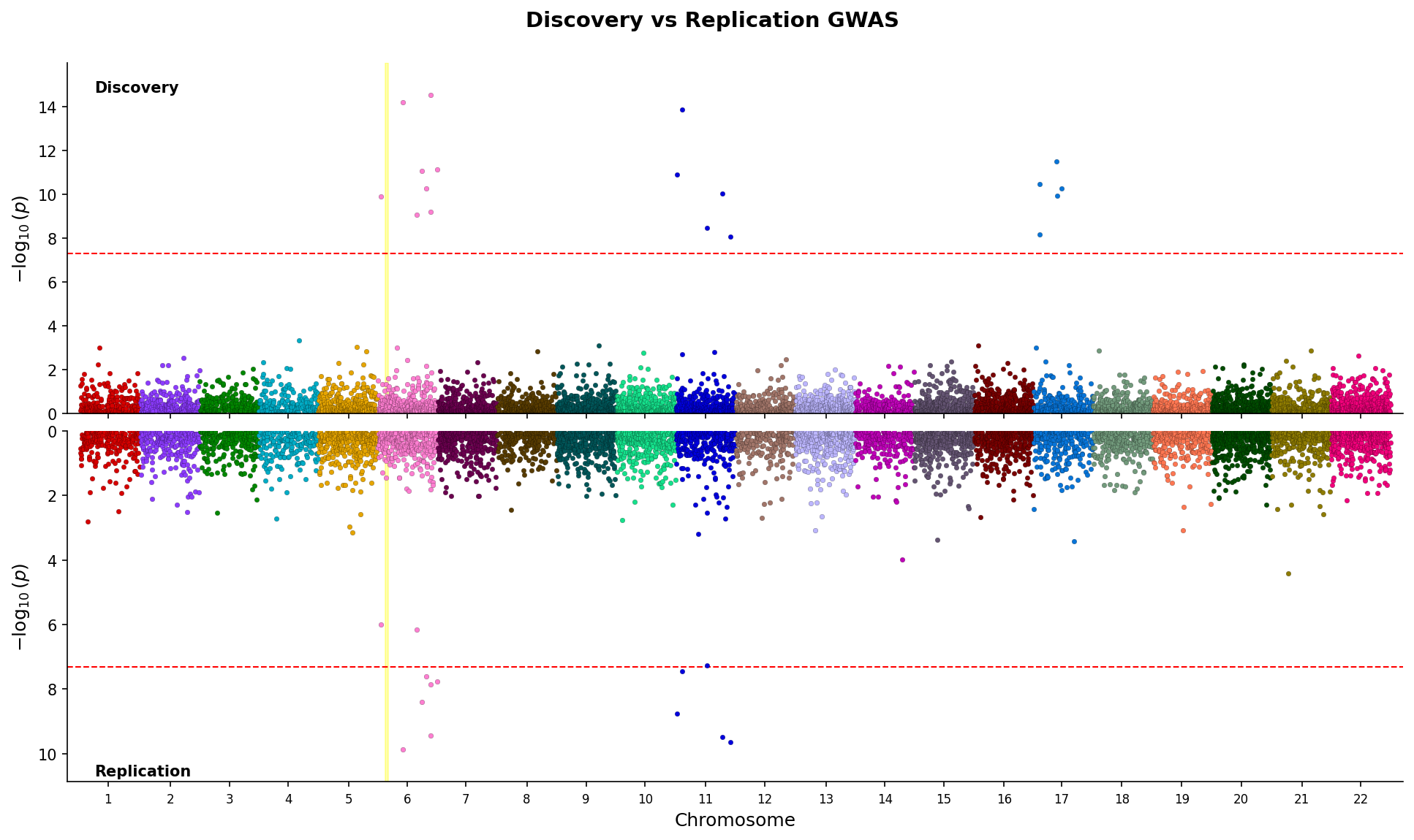
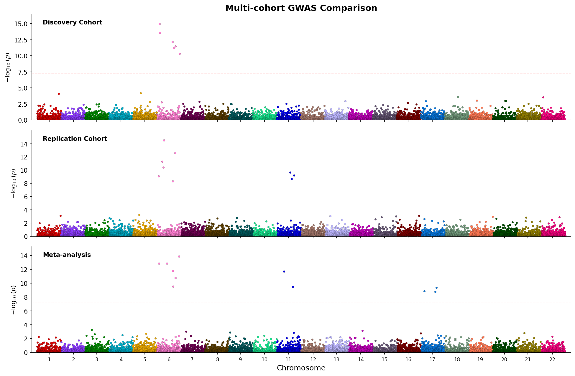
+3. **Miami plots**: Mirrored Manhattan plots for comparing two GWAS datasets (discovery vs replication)
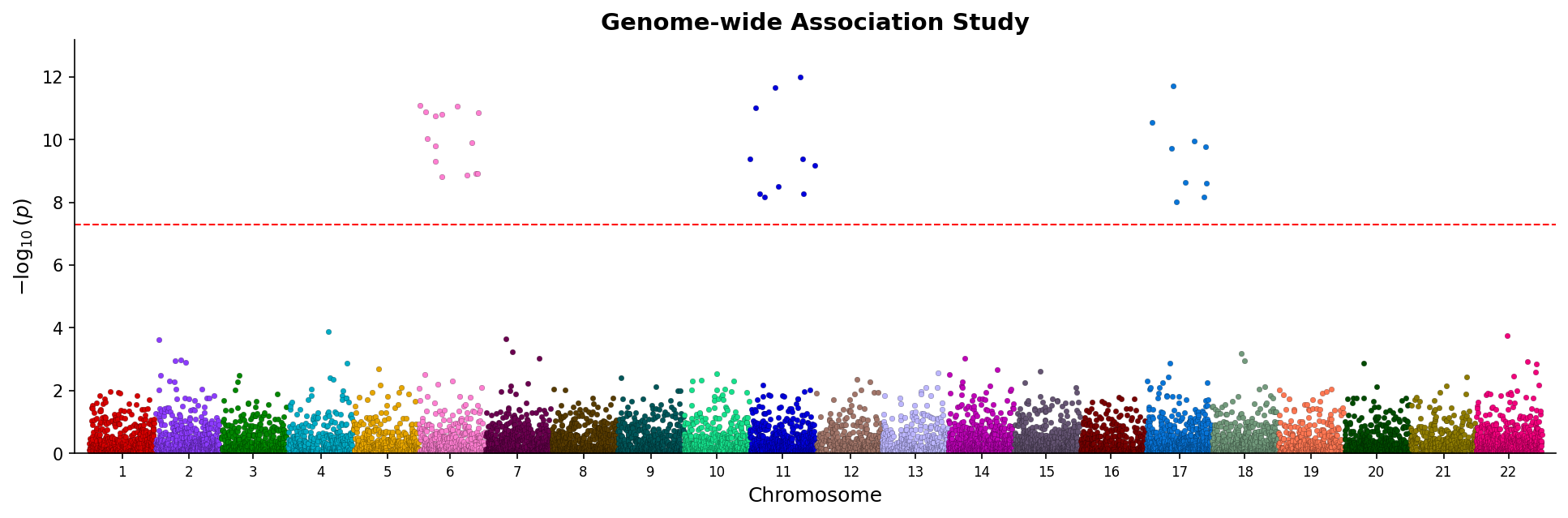
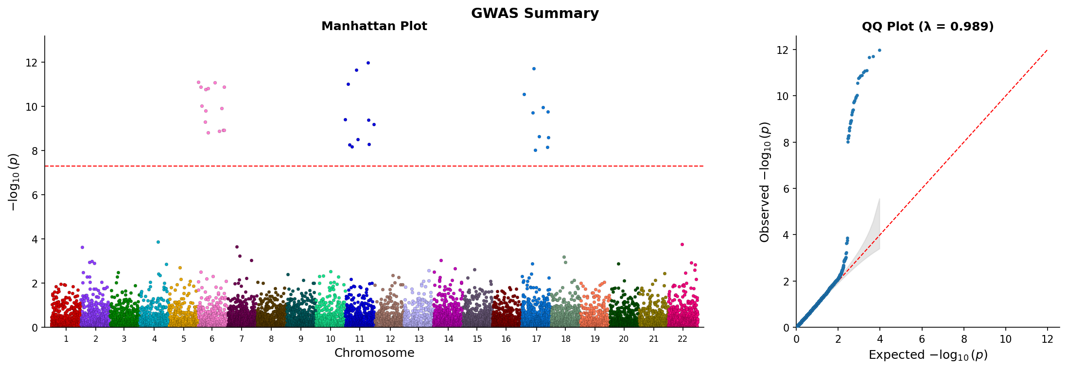
+4. **Manhattan plots**: Genome-wide association visualization with chromosome coloring
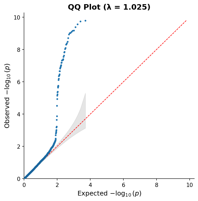
+5. **QQ plots**: Quantile-quantile plots with confidence bands and genomic inflation factor
+6. **eQTL plot**: Expression QTL data aligned with association plots and gene tracks
+7. **Fine-mapping plots**: Visualize SuSiE credible sets with posterior inclusion probabilities
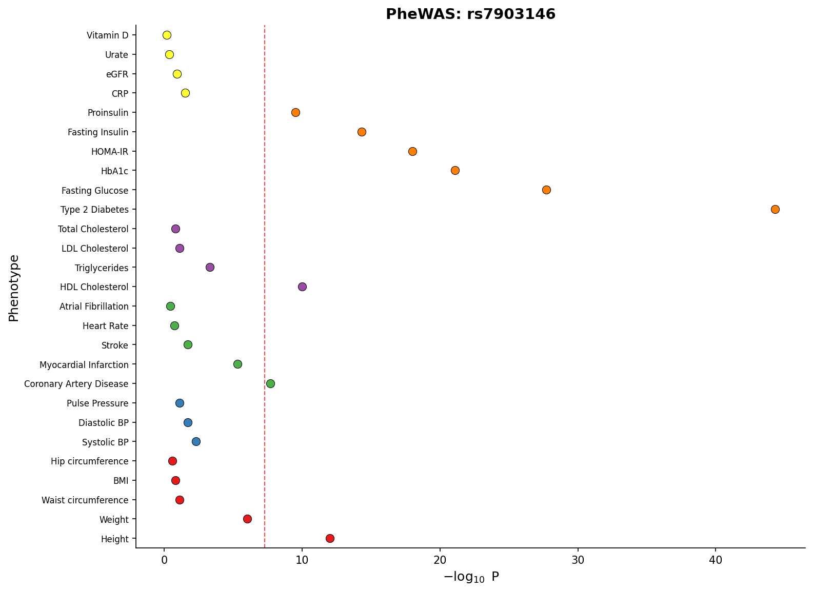
+8. **PheWAS plots**: Phenome-wide association study visualization across multiple phenotypes
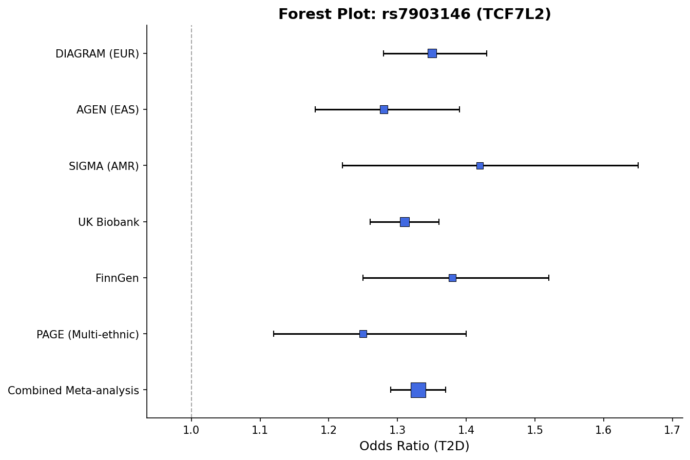
+9. **Forest plots**: Meta-analysis effect size visualization with confidence intervals
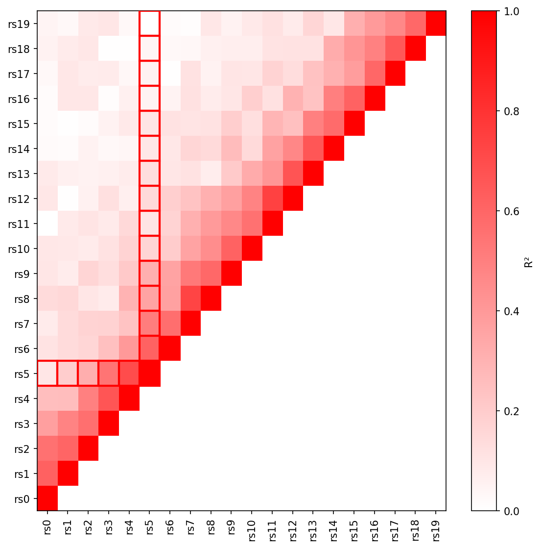
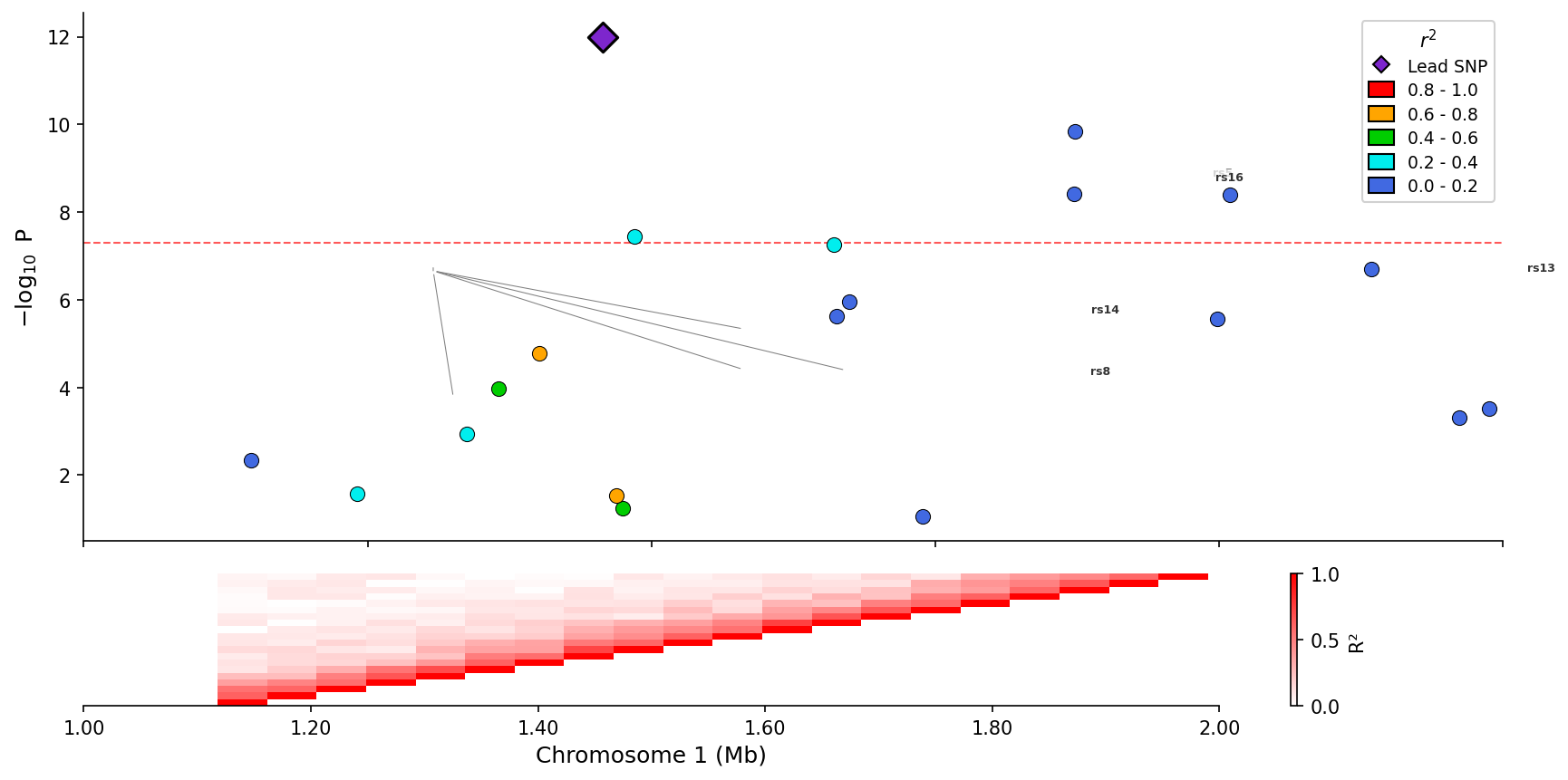
+10. **LD heatmaps**: Triangular heatmaps showing pairwise LD patterns, standalone or integrated below regional plots
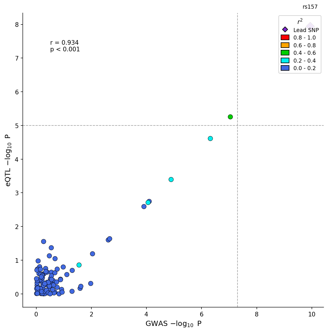
+11. **Colocalization plots**: GWAS-eQTL scatter plots with LD coloring, correlation statistics, and effect direction visualization
+12. **Multiple backends**: matplotlib (publication-ready), plotly (interactive), bokeh (dashboard integration)
+12. **Pandas and PySpark support**: Works with both Pandas and PySpark DataFrames for large-scale genomics data
+13. **Convenience data file loaders**: Load and validate common GWAS, eQTL and fine-mapping file formats
+14. **Automatic gene annotations**: Fetch gene/exon data from Ensembl REST API with caching (human, mouse, rat, canine, feline, and any Ensembl species)
 
 ## Installation
 
@@ -255,7 +258,7 @@ fig = plotter.plot_stacked(
 )
 ```
 
-![Example stacked plot comparing two phenotypes](https://raw.githubusercontent.com/michael-denyer/pyLocusZoom/main/examples/stacked_plot.png)
+![Example stacked plot comparing two phenotypes](https://raw.githubusercontent.com/michael-denyer/pyLocusZoom/main/examples/matplotlib/stacked_plot.png)
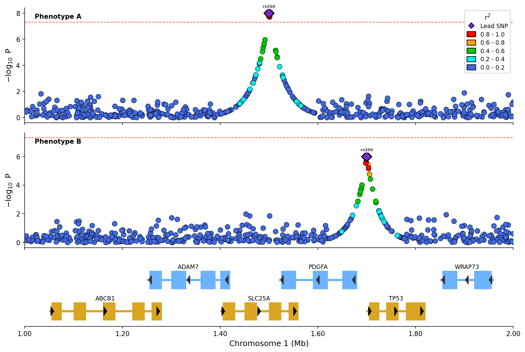
 *Stacked plot comparing two phenotypes with LD coloring and shared gene track.*
 
 ## eQTL Overlay
@@ -284,7 +287,7 @@ fig = plotter.plot_stacked(
 )
 ```
 
-![Example eQTL overlay plot](https://raw.githubusercontent.com/michael-denyer/pyLocusZoom/main/examples/eqtl_overlay.png)
+![Example eQTL overlay plot](https://raw.githubusercontent.com/michael-denyer/pyLocusZoom/main/examples/matplotlib/eqtl_overlay.png)
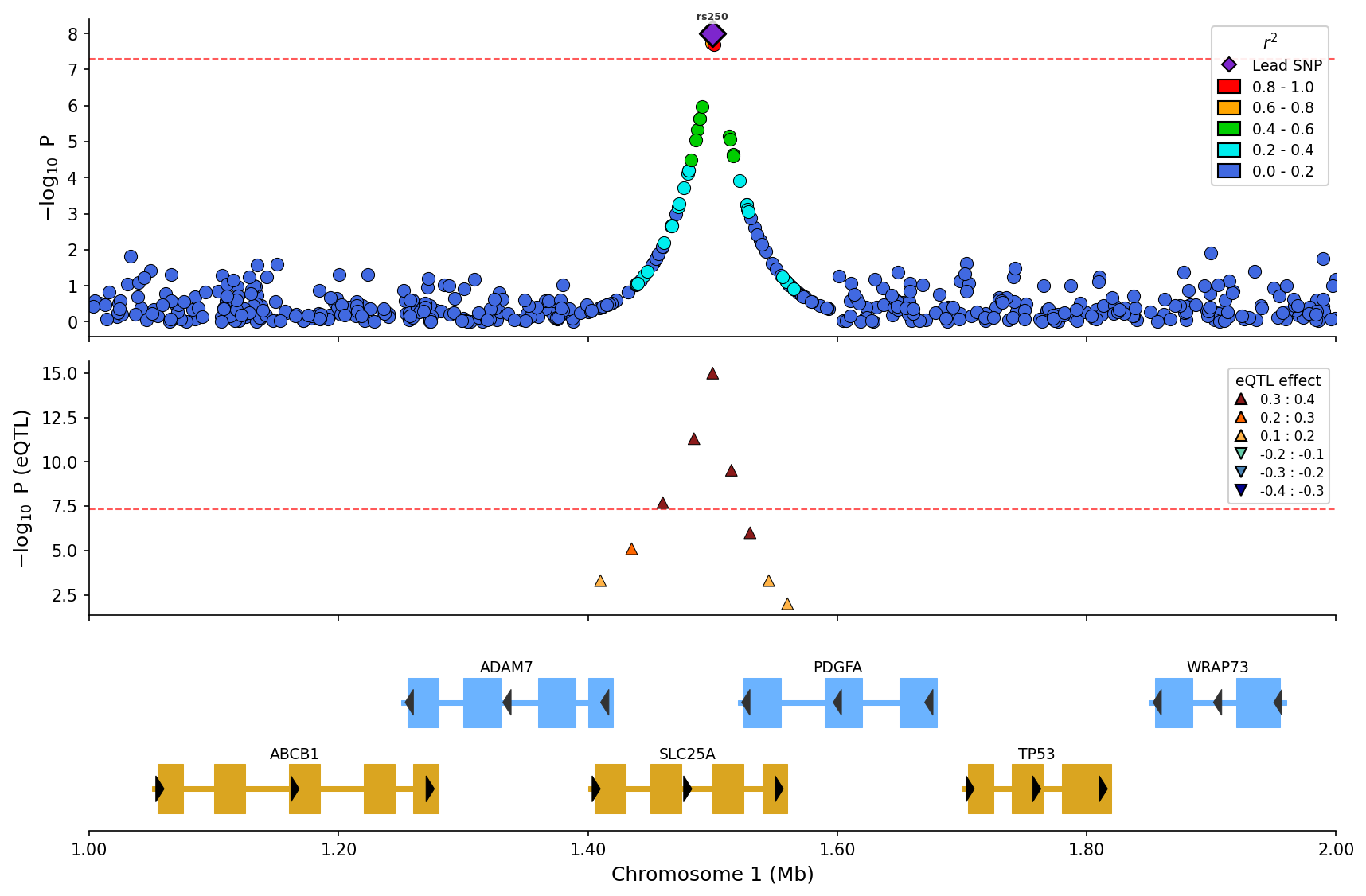
 *eQTL overlay with effect direction (up/down triangles) and magnitude binning.*
 
 ## Fine-mapping Visualization
@@ -313,9 +316,108 @@ fig = plotter.plot_stacked(
 )
 ```
 
-![Example fine-mapping plot](https://raw.githubusercontent.com/michael-denyer/pyLocusZoom/main/examples/finemapping_plot.png)
+![Example fine-mapping plot](https://raw.githubusercontent.com/michael-denyer/pyLocusZoom/main/examples/matplotlib/finemapping_plot.png)
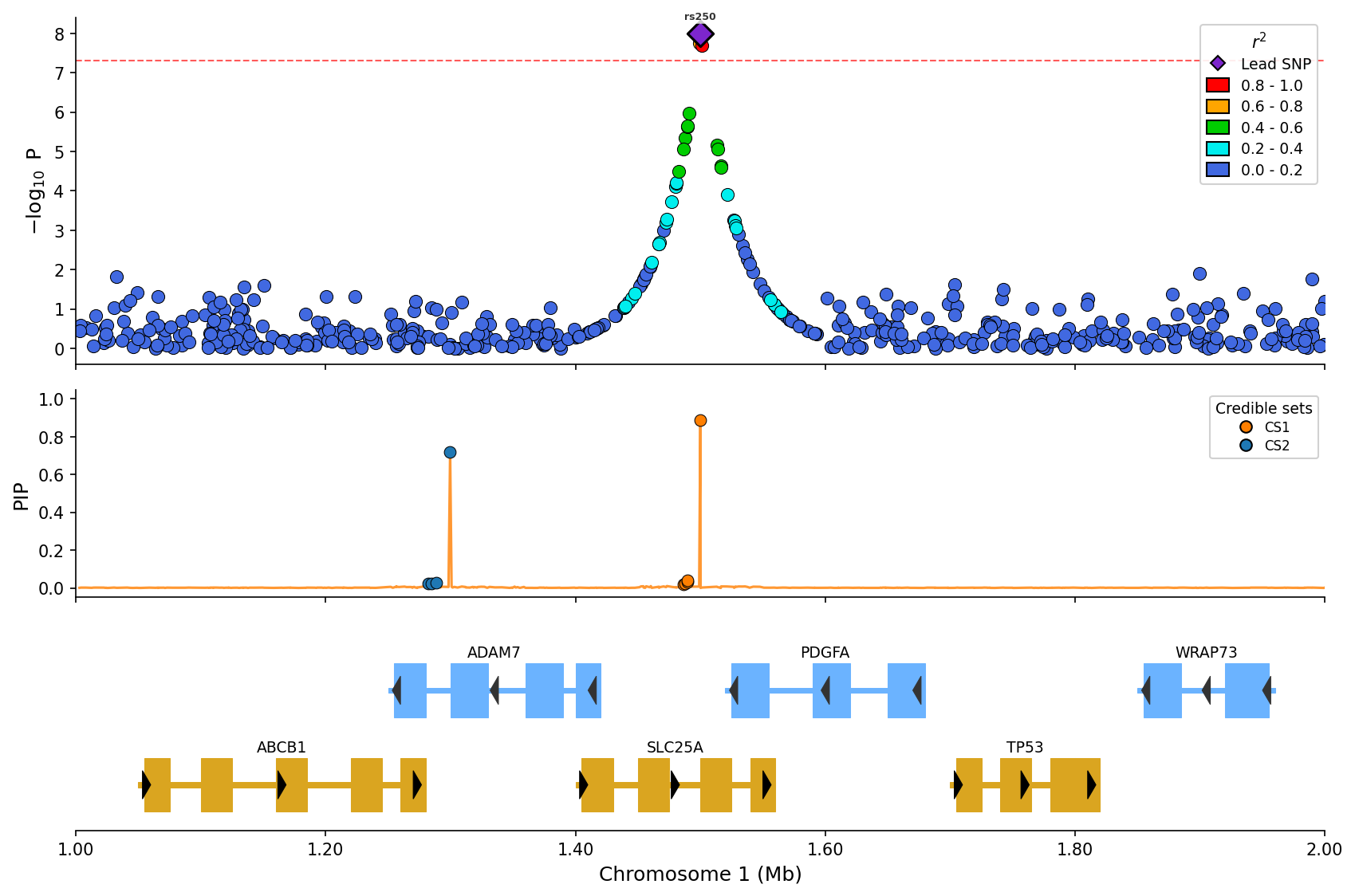
 *Fine-mapping visualization with PIP line and credible set coloring (CS1/CS2).*
 
+## LD Heatmaps
+
+Create triangular LD heatmaps showing pairwise linkage disequilibrium patterns:
+
+```python
+from pylocuszoom import LDHeatmapPlotter
+
+# ld_matrix is a square DataFrame with SNP IDs as index/columns
+# snp_ids is a list of SNP IDs in the matrix
+
+ld_plotter = LDHeatmapPlotter()
+fig = ld_plotter.plot(
+    ld_matrix,
+    snp_ids,
+    highlight_snp_id="rs12345",  # Highlight lead SNP
+    metric="r2",                  # or "dprime"
+)
+fig.savefig("ld_heatmap.png", dpi=150)
+```
+
+![Example LD heatmap](https://raw.githubusercontent.com/michael-denyer/pyLocusZoom/main/examples/matplotlib/ld_heatmap.png)
+*Triangular LD heatmap with R² values and lead SNP highlighted.*
+
+### Integrated LD Heatmap with Regional Plot
+
+Add an LD heatmap panel below a regional association plot:
+
+```python
+from pylocuszoom import LocusZoomPlotter
+
+plotter = LocusZoomPlotter(species="canine")
+
+fig = plotter.plot(
+    gwas_df,
+    chrom=1,
+    start=1000000,
+    end=2000000,
+    lead_pos=1500000,
+    ld_heatmap_df=ld_matrix,         # Pairwise LD matrix
+    ld_heatmap_snp_ids=snp_ids,      # SNP IDs in matrix
+    ld_heatmap_height=0.25,          # Panel height ratio
+)
+```
+
+![Example regional plot with LD heatmap](https://raw.githubusercontent.com/michael-denyer/pyLocusZoom/main/examples/matplotlib/regional_with_ld_heatmap.png)
+*Regional association plot with integrated LD heatmap panel below.*
+
+## Colocalization Plots
+
+Visualize GWAS-eQTL colocalization by comparing association signals in a scatter plot with LD coloring:
+
+```python
+from pylocuszoom import ColocPlotter
+
+# GWAS and eQTL data with matching positions
+gwas_df = pd.DataFrame({
+    "pos": positions,
+    "p": gwas_pvalues,
+    "ld_r2": ld_values,  # Optional: LD with lead SNP
+})
+
+eqtl_df = pd.DataFrame({
+    "pos": positions,
+    "p": eqtl_pvalues,
+})
+
+plotter = ColocPlotter()
+fig = plotter.plot_coloc(
+    gwas_df=gwas_df,
+    eqtl_df=eqtl_df,
+    pos_col="pos",
+    gwas_p_col="p",
+    eqtl_p_col="p",
+    ld_col="ld_r2",
+    gwas_threshold=5e-8,
+    eqtl_threshold=1e-5,
+)
+fig.savefig("colocalization.png", dpi=150)
+```
+
+![Example colocalization plot](https://raw.githubusercontent.com/michael-denyer/pyLocusZoom/main/examples/matplotlib/colocalization_plot.png)
+*GWAS-eQTL colocalization scatter plot with LD coloring and correlation statistics.*
+
+**Advanced options** include effect direction coloring and H4 posterior probability display:
+
+```python
+fig = plotter.plot_coloc(
+    gwas_df=gwas_df,
+    eqtl_df=eqtl_df,
+    pos_col="pos",
+    gwas_p_col="p",
+    eqtl_p_col="p",
+    gwas_effect_col="beta",
+    eqtl_effect_col="slope",
+    color_by_effect=True,  # Green=congruent, Red=incongruent
+    h4_posterior=0.85,     # Display coloc H4 probability
+)
+```
+
 ## PheWAS Plots
 
 Visualize associations of a single variant across multiple phenotypes:
@@ -337,7 +439,7 @@ fig = stats_plotter.plot_phewas(
 )
 ```
 
-![Example PheWAS plot](https://raw.githubusercontent.com/michael-denyer/pyLocusZoom/main/examples/phewas_plot.png)
+![Example PheWAS plot](https://raw.githubusercontent.com/michael-denyer/pyLocusZoom/main/examples/matplotlib/phewas_plot.png)
 *PheWAS plot showing associations across phenotype categories with significance threshold.*
 
 ## Forest Plots
@@ -363,9 +465,52 @@ fig = stats_plotter.plot_forest(
 )
 ```
 
-![Example forest plot](https://raw.githubusercontent.com/michael-denyer/pyLocusZoom/main/examples/forest_plot.png)
+![Example forest plot](https://raw.githubusercontent.com/michael-denyer/pyLocusZoom/main/examples/matplotlib/forest_plot.png)
 *Forest plot with effect sizes, confidence intervals, and weight-proportional markers.*
 
+## Miami Plots
+
+Compare two GWAS datasets with mirrored Manhattan plots (top panel ascending, bottom panel inverted):
+
+```python
+from pylocuszoom import MiamiPlotter
+
+plotter = MiamiPlotter(species="human")
+
+fig = plotter.plot_miami(
+    discovery_df,
+    replication_df,
+    chrom_col="chrom",
+    pos_col="pos",
+    p_col="p",
+    top_label="Discovery",
+    bottom_label="Replication",
+    top_threshold=5e-8,
+    bottom_threshold=1e-6,
+    highlight_regions=[("6", 30_000_000, 35_000_000)],  # Highlight MHC region
+)
+fig.savefig("miami.png", dpi=150)
+```
+
+**Interactive backends** (Plotly/Bokeh) provide hover tooltips showing SNP details:
+
+```python
+# Plotly - interactive HTML with hover tooltips
+plotter = MiamiPlotter(species="human", backend="plotly")
+fig = plotter.plot_miami(discovery_df, replication_df, ...)
+fig.write_html("miami_interactive.html")
+
+# Bokeh - dashboard-ready interactive plots
+from bokeh.io import output_file, save
+plotter = MiamiPlotter(species="human", backend="bokeh")
+fig = plotter.plot_miami(discovery_df, replication_df, ...)
+output_file("miami_bokeh.html")
+save(fig)
+```
+
+![Example Miami plot](https://raw.githubusercontent.com/michael-denyer/pyLocusZoom/main/examples/matplotlib/miami_plot.png)
+*Miami plot comparing discovery and replication GWAS with mirrored y-axes and region highlighting.*
+
 ## Manhattan Plots
 
 Create genome-wide Manhattan plots showing associations across all chromosomes:
@@ -386,7 +531,7 @@ fig = plotter.plot_manhattan(
 fig.savefig("manhattan.png", dpi=150)
 ```
 
-![Example Manhattan plot](https://raw.githubusercontent.com/michael-denyer/pyLocusZoom/main/examples/manhattan_plot.png)
+![Example Manhattan plot](https://raw.githubusercontent.com/michael-denyer/pyLocusZoom/main/examples/matplotlib/manhattan_plot.png)
 *Manhattan plot showing genome-wide associations with chromosome coloring and significance threshold.*
 
 Categorical Manhattan plots (PheWAS-style) are also supported:
@@ -418,7 +563,7 @@ fig = plotter.plot_qq(
 fig.savefig("qq_plot.png", dpi=150)
 ```
 
-![Example QQ plot](https://raw.githubusercontent.com/michael-denyer/pyLocusZoom/main/examples/qq_plot.png)
+![Example QQ plot](https://raw.githubusercontent.com/michael-denyer/pyLocusZoom/main/examples/matplotlib/qq_plot.png)
 *QQ plot with 95% confidence band and genomic inflation factor (λ).*
 
 ## Stacked Manhattan Plots
@@ -443,7 +588,7 @@ fig = plotter.plot_manhattan_stacked(
 fig.savefig("manhattan_stacked.png", dpi=150)
 ```
 
-![Example stacked Manhattan plot](https://raw.githubusercontent.com/michael-denyer/pyLocusZoom/main/examples/manhattan_stacked.png)
+![Example stacked Manhattan plot](https://raw.githubusercontent.com/michael-denyer/pyLocusZoom/main/examples/matplotlib/manhattan_stacked.png)
 *Stacked Manhattan plots comparing three GWAS studies with shared chromosome axis.*
 
 ## Manhattan and QQ Side-by-Side
@@ -469,7 +614,7 @@ fig = plotter.plot_manhattan_qq(
 fig.savefig("manhattan_qq.png", dpi=150)
 ```
 
-![Example Manhattan and QQ side-by-side](https://raw.githubusercontent.com/michael-denyer/pyLocusZoom/main/examples/manhattan_qq_sidebyside.png)
+![Example Manhattan and QQ side-by-side](https://raw.githubusercontent.com/michael-denyer/pyLocusZoom/main/examples/matplotlib/manhattan_qq_sidebyside.png)
 *Combined Manhattan and QQ plot showing genome-wide associations and p-value distribution.*
 
 ## PySpark Support

{pylocuszoom-1.2.0.dist-info → pylocuszoom-1.3.1.dist-info}/RECORD

@@ -1,21 +1,25 @@
-pylocuszoom/__init__.py,sha256=l_P-moa2FZkrqvpyRj_PT97Q70X7l29bCjzNB5NI_mM,6204
+pylocuszoom/__init__.py,sha256=VwZBIjjY-k6oQVkSgcsAwTkDitHdaHRe2gDUZ5b1YhA,6599
 pylocuszoom/_plotter_utils.py,sha256=ELdSOcKk2KvOo_AxEWHeutmmUS4zZMaDMmQfpQUWaF0,1541
-pylocuszoom/colors.py,sha256=B28rfhWwGZ-e6Q-F43iXxC6NZpjUo0yWk4S_-vp9ZvU,7686
-pylocuszoom/config.py,sha256=qjIEodI-RY71RVyQ5QmE6WXcPXU4Re_xEWiDlkEww3g,13266
+pylocuszoom/coloc.py,sha256=ND56BgUp_yLDTak2RsD9OqZK-X93eDGkL9Q97C2_Fz0,2191
+pylocuszoom/coloc_plotter.py,sha256=9q76_4mYLNU6PjVw_rqx2THdTleI9U6mpzGBA6PnfrY,14036
+pylocuszoom/colors.py,sha256=j1qBHHNTIE9k4bAkIrl7B7bTpTQdWq34-DdJ_y7hZPk,8751
+pylocuszoom/config.py,sha256=Ow8YiW5Yl801K71jOnrPivHvAbA58uH1BvCAbV9hojM,16008
 pylocuszoom/ensembl.py,sha256=w2msgBoIrY79iHI3hURSbevvdFHxHyWF9Z78hXtAaBc,14296
 pylocuszoom/eqtl.py,sha256=9hGcFARABQRCMN3rco0pVlFJdmlh4SLBBKSgOvdIH_U,5924
 pylocuszoom/exceptions.py,sha256=nd-rWMUodW62WVV4TfcYVPQcb66xV6v9FA-_4xHb5VY,926
 pylocuszoom/finemapping.py,sha256=S3ulQj3fkaDM3n4I8EBymbWym_kTD5NEqfIEj93Mdjk,9630
 pylocuszoom/forest.py,sha256=K-wBinxBOqIzsNMtZJ587e_oMhUXIXEqmEzVTUbmHSY,1161
 pylocuszoom/gene_track.py,sha256=Sh0JCSdLNAAH0NQEiDVMvyXjm63PiCMq3gLvewcagvo,17277
-pylocuszoom/labels.py,sha256=l4PHAR_err75Z9kTmb3a2h0eunkFj6UjzhKBUgmZTDc,3623
-pylocuszoom/ld.py,sha256=64xIulpDVvbMSryWUPoCQ99Odcjwf1wejpwVr_30MLU,6412
+pylocuszoom/labels.py,sha256=RPgEcCGPA2VQ1rXIW3WYy0AQ0EE0VBzbh_4EkhsWsNc,4343
+pylocuszoom/ld.py,sha256=CphRau26XL9MoHiU3qRXlSz1Eg39TJt7MNIPZSZDr8M,13999
+pylocuszoom/ld_heatmap_plotter.py,sha256=siHKL-tq7qQBTgyfH09uL0YJPmOGxG3udq8p1We5p0I,8373
 pylocuszoom/loaders.py,sha256=KpWPBO0BCb2yrGTtgdiOqOuhx2YLmjK_ywmpr3onnx8,25156
 pylocuszoom/logging.py,sha256=nZHEkbnjp8zoyWj_S-Hy9UQvUYLoMoxyiOWRozBT2dg,4987
 pylocuszoom/manhattan.py,sha256=sNhPnsfsIqe1ls74D-kKMFyF_ZmaYB9Ul8qf4UMWnF0,8022
 pylocuszoom/manhattan_plotter.py,sha256=1QQxaXEh5YG4x6ZIxpdhdfQPI2KuO_525qYKI7c32n4,27584
+pylocuszoom/miami_plotter.py,sha256=J7GcgeIKyJvJTpQQHx9YNwH5NzpYSej2HPFSGu5YeLY,18099
 pylocuszoom/phewas.py,sha256=6g2LmwA5kmxYlHgPxJvuXIMerEqfqgsrth110Y3CgVU,968
-pylocuszoom/plotter.py,sha256=Z24UWRRdp9E-nJx2urKmM_jz-i0OZ9BOwSmJJestdS4,42362
+pylocuszoom/plotter.py,sha256=I6fktn1mwE-ZM6bnKUqXrdN_eMQ6oHGaJBq9DwoT4xI,60488
 pylocuszoom/py.typed,sha256=47DEQpj8HBSa-_TImW-5JCeuQeRkm5NMpJWZG3hSuFU,0
 pylocuszoom/qq.py,sha256=GPIFHXYCLvhP4IUgjcU3QELLREH8r1AEYXMord8gtEo,3650
 pylocuszoom/recombination.py,sha256=M-wDBdGbC5qGDHPFoGzBTPmTdiRD7bpRskyxBAKxTUY,15878
@@ -24,13 +28,13 @@ pylocuszoom/stats_plotter.py,sha256=67bgU-TXGnmVTxfTRWT3-PFemVVy6lTu4-ZlxUnwHS4,
 pylocuszoom/utils.py,sha256=Z2P__Eau3ilF2ftuAZBm11EZ1NqCFQzfr4br9jCiJmg,6887
 pylocuszoom/validation.py,sha256=3D9axjUvNXWW3Mk7dwRG38-di2P0zDpVVGF5WNSfZbk,7403
 pylocuszoom/backends/__init__.py,sha256=xefVj3jVxmYwVLLY5AZtFqTPMehQxZ2qGd-Pk7_V_Bk,4267
-pylocuszoom/backends/base.py,sha256=d_IqH2yGWIfQHeUCcavV4eL6V68hpNtOyGfTyb2ke0I,22628
-pylocuszoom/backends/bokeh_backend.py,sha256=cubjEzNq5vHov-CeBMLgmf3SAtEET-fUUB8d_oYFgiw,29151
+pylocuszoom/backends/base.py,sha256=Wgzr6ncKnqZpjEYrc6aPmIKDWdZLm18mMO7q7XRU6SA,25640
+pylocuszoom/backends/bokeh_backend.py,sha256=ft0W5ScxPoA6T6GB7k9PFfTMgOCyFom_plqVItdaUA0,34198
 pylocuszoom/backends/hover.py,sha256=Hjm_jcxJL8dDxO_Ye7jeWAUcHKlbH6oO8ZfGJ2MzIFM,6564
-pylocuszoom/backends/matplotlib_backend.py,sha256=9WAFLWcclj2-4WKi6bE6IPJfQ_HNoIekOE45ibBGPa0,22824
-pylocuszoom/backends/plotly_backend.py,sha256=VDEZMdP7nOeFYLli-YOc_2DG00ZA6VVRNUcvT5PU0HM,39084
+pylocuszoom/backends/matplotlib_backend.py,sha256=SKTL_6QCc2D_UVITH543O-zPD_I8AwDLCZE0Re0KfE0,27269
+pylocuszoom/backends/plotly_backend.py,sha256=cow67G8dIcrxSI3XOPFWJ9hSLqe1-MB4NFSeO8GDRG4,42228
 pylocuszoom/reference_data/__init__.py,sha256=qqHqAUt1jebGlCN3CjqW3Z-_coHVNo5K3a3bb9o83hA,109
-pylocuszoom-1.2.0.dist-info/METADATA,sha256=O0SkzFPHNYqOrjh0zUfL_73UvE2z2NzzH1nKYECchw4,22488
-pylocuszoom-1.2.0.dist-info/WHEEL,sha256=WLgqFyCfm_KASv4WHyYy0P3pM_m7J5L9k2skdKLirC8,87
-pylocuszoom-1.2.0.dist-info/licenses/LICENSE.md,sha256=U2y_hv8RcN5lECA3uK88irU3ODUE1TDAPictcmnP0Q4,698
-pylocuszoom-1.2.0.dist-info/RECORD,,
+pylocuszoom-1.3.1.dist-info/METADATA,sha256=nHe6YBAHx718EndDz71xIukqf_WwJ7Q4yERBkgz9xmo,27020
+pylocuszoom-1.3.1.dist-info/WHEEL,sha256=WLgqFyCfm_KASv4WHyYy0P3pM_m7J5L9k2skdKLirC8,87
+pylocuszoom-1.3.1.dist-info/licenses/LICENSE.md,sha256=bqhD2fIhoqfLdX1lyGNoufIHWE7Q8mU-SyFadwKn4cc,34902
+pylocuszoom-1.3.1.dist-info/RECORD,,