pyEllipse 0.1.2__py3-none-any.whl
This diff represents the content of publicly available package versions that have been released to one of the supported registries. The information contained in this diff is provided for informational purposes only and reflects changes between package versions as they appear in their respective public registries.
- pyEllipse/__init__.py +31 -0
- pyEllipse/confidence_ellipse.py +248 -0
- pyEllipse/hotelling_coordinates.py +164 -0
- pyEllipse/hotelling_parameters.py +221 -0
- pyellipse-0.1.2.dist-info/METADATA +313 -0
- pyellipse-0.1.2.dist-info/RECORD +8 -0
- pyellipse-0.1.2.dist-info/WHEEL +4 -0
- pyellipse-0.1.2.dist-info/licenses/LICENSE +21 -0
pyEllipse/__init__.py
ADDED
|
@@ -0,0 +1,31 @@
|
|
|
1
|
+
"""
|
|
2
|
+
**Statistical confidence ellipses and Hotelling's T-squared statistic**
|
|
3
|
+
|
|
4
|
+
The pyEllipse library provides robust computational tools for generating and analyzing
|
|
5
|
+
confidence ellipses and ellipsoids in multivariate datasets. Built on rigorous statistical
|
|
6
|
+
foundations, it supports both classical normal-based confidence regions and Hotelling's
|
|
7
|
+
T-squared ellipses, delivering robust uncertainty quantification for small samples, outlier
|
|
8
|
+
detection, process control, and high-dimensional data exploration.
|
|
9
|
+
"""
|
|
10
|
+
|
|
11
|
+
# Import main functions with their proper names
|
|
12
|
+
from .hotelling_parameters import hotelling_parameters
|
|
13
|
+
from .hotelling_coordinates import hotelling_coordinates
|
|
14
|
+
from .confidence_ellipse import confidence_ellipse
|
|
15
|
+
|
|
16
|
+
__all__ = [
|
|
17
|
+
"hotelling_parameters",
|
|
18
|
+
"hotelling_coordinates",
|
|
19
|
+
"confidence_ellipse",
|
|
20
|
+
]
|
|
21
|
+
|
|
22
|
+
# Library metadata
|
|
23
|
+
__title__ = "pyEllipse"
|
|
24
|
+
__description__ = "Statistical confidence ellipses and Hotelling's T-squared ellipses"
|
|
25
|
+
__url__ = "https://github.com/ChristianGoueguel/pyEllipse"
|
|
26
|
+
__license__ = "MIT"
|
|
27
|
+
__version__ = "0.1.1"
|
|
28
|
+
__author__ = "Christian L. Goueguel"
|
|
29
|
+
__maintainer__ = "Christian L. Goueguel"
|
|
30
|
+
__credits__ = ["Christian L. Goueguel"]
|
|
31
|
+
__email__ = "christian.goueguel@gmail.com"
|
|
@@ -0,0 +1,248 @@
|
|
|
1
|
+
"""
|
|
2
|
+
**Module to compute coordinate points for confidence regions based on
|
|
3
|
+
normal or Hotelling's T-squared distributions**
|
|
4
|
+
"""
|
|
5
|
+
import numpy as np
|
|
6
|
+
import pandas as pd
|
|
7
|
+
from scipy import stats
|
|
8
|
+
from typing import Optional, Literal
|
|
9
|
+
import warnings
|
|
10
|
+
|
|
11
|
+
|
|
12
|
+
def confidence_ellipse(
|
|
13
|
+
data: pd.DataFrame,
|
|
14
|
+
x: str,
|
|
15
|
+
y: str,
|
|
16
|
+
z: Optional[str] = None,
|
|
17
|
+
group_by: Optional[str] = None,
|
|
18
|
+
conf_level: float = 0.95,
|
|
19
|
+
robust: bool = False,
|
|
20
|
+
distribution: Literal["normal", "hotelling"] = "normal"
|
|
21
|
+
) -> pd.DataFrame:
|
|
22
|
+
"""
|
|
23
|
+
This module generates coordinate points for visualizing confidence regions in multivariate data.
|
|
24
|
+
It supports both 2D confidence ellipses and 3D confidence ellipsoids at user-specified
|
|
25
|
+
confidence levels, with options for normal distribution assumptions or Hotelling's T-squared
|
|
26
|
+
distribution for small sample sizes.
|
|
27
|
+
|
|
28
|
+
Parameters
|
|
29
|
+
----------
|
|
30
|
+
* `data` : Input data frame containing the variables.
|
|
31
|
+
|
|
32
|
+
* `x` : Column name for the x-axis variable.
|
|
33
|
+
|
|
34
|
+
* `y` : Column name for the y-axis variable.
|
|
35
|
+
|
|
36
|
+
* `z` : Column name for the z-axis variable (None by default).
|
|
37
|
+
If provided, computes a 3D ellipsoid instead of a 2D ellipse.
|
|
38
|
+
|
|
39
|
+
* `group_by` : Column name for the grouping variable (None by default).
|
|
40
|
+
This grouping variable should be categorical.
|
|
41
|
+
|
|
42
|
+
* `conf_level` : Confidence level for the ellipse/ellipsoid (between 0 and 1).
|
|
43
|
+
|
|
44
|
+
* `robust` : When `True`, uses robust estimation methods for location and scale.
|
|
45
|
+
Uses sklearn's `EllipticEnvelope` for robust covariance estimation.
|
|
46
|
+
|
|
47
|
+
* `distribution` : Distribution used to calculate the quantile for the ellipse.
|
|
48
|
+
Options are:
|
|
49
|
+
|
|
50
|
+
- `'normal'`: Uses chi-square distribution (appropriate for large samples)
|
|
51
|
+
- `'hotelling'`: Uses Hotelling's T² distribution (better for small samples)
|
|
52
|
+
|
|
53
|
+
Returns
|
|
54
|
+
-------
|
|
55
|
+
DataFrame containing the coordinate points:
|
|
56
|
+
|
|
57
|
+
- For 2D: columns 'x' and 'y'
|
|
58
|
+
- For 3D: columns 'x', 'y', and 'z'
|
|
59
|
+
If group_by is specified, includes the grouping column.
|
|
60
|
+
"""
|
|
61
|
+
if not isinstance(data, pd.DataFrame):
|
|
62
|
+
raise TypeError("Input 'data' must be a pandas DataFrame.")
|
|
63
|
+
|
|
64
|
+
if x not in data.columns:
|
|
65
|
+
raise ValueError(f"Column '{x}' not found in data.")
|
|
66
|
+
|
|
67
|
+
if y not in data.columns:
|
|
68
|
+
raise ValueError(f"Column '{y}' not found in data.")
|
|
69
|
+
|
|
70
|
+
if not isinstance(conf_level, (int, float)):
|
|
71
|
+
raise TypeError("'conf_level' must be numeric.")
|
|
72
|
+
|
|
73
|
+
if conf_level <= 0 or conf_level >= 1:
|
|
74
|
+
raise ValueError("'conf_level' must be between 0 and 1.")
|
|
75
|
+
|
|
76
|
+
if distribution not in ["normal", "hotelling"]:
|
|
77
|
+
raise ValueError("'distribution' must be either 'normal' or 'hotelling'.")
|
|
78
|
+
|
|
79
|
+
if z is None:
|
|
80
|
+
# 2D ellipse
|
|
81
|
+
if group_by is None:
|
|
82
|
+
selected_data = data[[x, y]].values
|
|
83
|
+
ellipse_coord = _transform_2d(selected_data, conf_level, robust, distribution)
|
|
84
|
+
result = pd.DataFrame(ellipse_coord, columns=['x', 'y'])
|
|
85
|
+
else:
|
|
86
|
+
if group_by not in data.columns:
|
|
87
|
+
raise ValueError(f"Column '{group_by}' not found in data.")
|
|
88
|
+
results = []
|
|
89
|
+
for group_name, group_data in data.groupby(group_by):
|
|
90
|
+
selected_data = group_data[[x, y]].values
|
|
91
|
+
ellipse_coord = _transform_2d(selected_data, conf_level, robust, distribution)
|
|
92
|
+
group_df = pd.DataFrame(ellipse_coord, columns=['x', 'y'])
|
|
93
|
+
group_df[group_by] = group_name
|
|
94
|
+
results.append(group_df)
|
|
95
|
+
result = pd.concat(results, ignore_index=True)
|
|
96
|
+
return result
|
|
97
|
+
else:
|
|
98
|
+
# 3D ellipsoid
|
|
99
|
+
if z not in data.columns:
|
|
100
|
+
raise ValueError(f"Column '{z}' not found in data.")
|
|
101
|
+
|
|
102
|
+
if group_by is None:
|
|
103
|
+
selected_data = data[[x, y, z]].values
|
|
104
|
+
ellipsoid_coord = _transform_3d(selected_data, conf_level, robust, distribution)
|
|
105
|
+
result = pd.DataFrame(ellipsoid_coord, columns=['x', 'y', 'z'])
|
|
106
|
+
else:
|
|
107
|
+
if group_by not in data.columns:
|
|
108
|
+
raise ValueError(f"Column '{group_by}' not found in data.")
|
|
109
|
+
results = []
|
|
110
|
+
for group_name, group_data in data.groupby(group_by):
|
|
111
|
+
selected_data = group_data[[x, y, z]].values
|
|
112
|
+
ellipsoid_coord = _transform_3d(selected_data, conf_level, robust, distribution)
|
|
113
|
+
group_df = pd.DataFrame(ellipsoid_coord, columns=['x', 'y', 'z'])
|
|
114
|
+
group_df[group_by] = group_name
|
|
115
|
+
results.append(group_df)
|
|
116
|
+
result = pd.concat(results, ignore_index=True)
|
|
117
|
+
return result
|
|
118
|
+
|
|
119
|
+
|
|
120
|
+
def _transform_2d(
|
|
121
|
+
x: np.ndarray,
|
|
122
|
+
conf_level: float,
|
|
123
|
+
robust: bool,
|
|
124
|
+
distribution: str
|
|
125
|
+
) -> np.ndarray:
|
|
126
|
+
"""
|
|
127
|
+
Transform 2D data to ellipse coordinates.
|
|
128
|
+
|
|
129
|
+
Parameters
|
|
130
|
+
----------
|
|
131
|
+
x : np.ndarray
|
|
132
|
+
2D array of shape (n_samples, 2)
|
|
133
|
+
conf_level : float
|
|
134
|
+
Confidence level
|
|
135
|
+
robust : bool
|
|
136
|
+
Whether to use robust estimation
|
|
137
|
+
distribution : str
|
|
138
|
+
Either 'normal' or 'hotelling'
|
|
139
|
+
|
|
140
|
+
Returns
|
|
141
|
+
-------
|
|
142
|
+
np.ndarray
|
|
143
|
+
Array of ellipse coordinates
|
|
144
|
+
"""
|
|
145
|
+
n = x.shape[0]
|
|
146
|
+
|
|
147
|
+
if n < 3:
|
|
148
|
+
raise ValueError("At least 3 observations are required.")
|
|
149
|
+
|
|
150
|
+
if not robust:
|
|
151
|
+
mean_vec = np.mean(x, axis=0)
|
|
152
|
+
cov_matrix = np.cov(x, rowvar=False)
|
|
153
|
+
else:
|
|
154
|
+
from sklearn.covariance import EllipticEnvelope
|
|
155
|
+
try:
|
|
156
|
+
robust_cov = EllipticEnvelope(support_fraction=0.9, random_state=42)
|
|
157
|
+
robust_cov.fit(x)
|
|
158
|
+
mean_vec = robust_cov.location_
|
|
159
|
+
cov_matrix = robust_cov.covariance_
|
|
160
|
+
except Exception as e:
|
|
161
|
+
warnings.warn(f"Robust estimation failed: {e}. Using classical estimates.")
|
|
162
|
+
mean_vec = np.mean(x, axis=0)
|
|
163
|
+
cov_matrix = np.cov(x, rowvar=False)
|
|
164
|
+
|
|
165
|
+
if np.any(np.isnan(cov_matrix)):
|
|
166
|
+
raise ValueError("Covariance matrix contains NA values.")
|
|
167
|
+
|
|
168
|
+
eigenvalues, eigenvectors = np.linalg.eigh(cov_matrix)
|
|
169
|
+
theta = np.linspace(0, 2 * np.pi, 361)
|
|
170
|
+
|
|
171
|
+
if distribution == "normal":
|
|
172
|
+
quantile = stats.chi2.ppf(conf_level, 2)
|
|
173
|
+
else: # hotelling
|
|
174
|
+
quantile = ((2 * (n - 1)) / (n - 2)) * stats.f.ppf(conf_level, 2, n - 2)
|
|
175
|
+
|
|
176
|
+
X = np.sqrt(eigenvalues[0] * quantile) * np.cos(theta)
|
|
177
|
+
Y = np.sqrt(eigenvalues[1] * quantile) * np.sin(theta)
|
|
178
|
+
R = np.column_stack([X, Y]) @ eigenvectors.T
|
|
179
|
+
result = R + mean_vec
|
|
180
|
+
return result
|
|
181
|
+
|
|
182
|
+
|
|
183
|
+
def _transform_3d(
|
|
184
|
+
x: np.ndarray,
|
|
185
|
+
conf_level: float,
|
|
186
|
+
robust: bool,
|
|
187
|
+
distribution: str
|
|
188
|
+
) -> np.ndarray:
|
|
189
|
+
"""
|
|
190
|
+
Transform 3D data to ellipsoid coordinates.
|
|
191
|
+
|
|
192
|
+
Parameters
|
|
193
|
+
----------
|
|
194
|
+
x : np.ndarray
|
|
195
|
+
3D array of shape (n_samples, 3)
|
|
196
|
+
conf_level : float
|
|
197
|
+
Confidence level
|
|
198
|
+
robust : bool
|
|
199
|
+
Whether to use robust estimation
|
|
200
|
+
distribution : str
|
|
201
|
+
Either 'normal' or 'hotelling'
|
|
202
|
+
|
|
203
|
+
Returns
|
|
204
|
+
-------
|
|
205
|
+
np.ndarray
|
|
206
|
+
Array of ellipsoid coordinates
|
|
207
|
+
"""
|
|
208
|
+
n = x.shape[0]
|
|
209
|
+
|
|
210
|
+
if n < 3:
|
|
211
|
+
raise ValueError("At least 3 observations are required.")
|
|
212
|
+
|
|
213
|
+
if not robust:
|
|
214
|
+
mean_vec = np.mean(x, axis=0)
|
|
215
|
+
cov_matrix = np.cov(x, rowvar=False)
|
|
216
|
+
else:
|
|
217
|
+
from sklearn.covariance import EllipticEnvelope
|
|
218
|
+
try:
|
|
219
|
+
robust_cov = EllipticEnvelope(support_fraction=0.9, random_state=42)
|
|
220
|
+
robust_cov.fit(x)
|
|
221
|
+
mean_vec = robust_cov.location_
|
|
222
|
+
cov_matrix = robust_cov.covariance_
|
|
223
|
+
except Exception as e:
|
|
224
|
+
warnings.warn(f"Robust estimation failed: {e}. Using classical estimates.")
|
|
225
|
+
mean_vec = np.mean(x, axis=0)
|
|
226
|
+
cov_matrix = np.cov(x, rowvar=False)
|
|
227
|
+
|
|
228
|
+
if np.any(np.isnan(cov_matrix)):
|
|
229
|
+
raise ValueError("Covariance matrix contains NA values.")
|
|
230
|
+
|
|
231
|
+
eigenvalues, eigenvectors = np.linalg.eigh(cov_matrix)
|
|
232
|
+
theta = np.linspace(0, 2 * np.pi, 50)
|
|
233
|
+
phi = np.linspace(0, np.pi, 50)
|
|
234
|
+
theta_grid, phi_grid = np.meshgrid(theta, phi)
|
|
235
|
+
theta_flat = theta_grid.flatten()
|
|
236
|
+
phi_flat = phi_grid.flatten()
|
|
237
|
+
|
|
238
|
+
if distribution == "normal":
|
|
239
|
+
quantile = stats.chi2.ppf(conf_level, 3)
|
|
240
|
+
else: # hotelling
|
|
241
|
+
quantile = ((3 * (n - 1)) / (n - 3)) * stats.f.ppf(conf_level, 3, n - 3)
|
|
242
|
+
|
|
243
|
+
X = np.sqrt(eigenvalues[0] * quantile) * np.sin(phi_flat) * np.cos(theta_flat)
|
|
244
|
+
Y = np.sqrt(eigenvalues[1] * quantile) * np.sin(phi_flat) * np.sin(theta_flat)
|
|
245
|
+
Z = np.sqrt(eigenvalues[2] * quantile) * np.cos(phi_flat)
|
|
246
|
+
R = np.column_stack([X, Y, Z]) @ eigenvectors.T
|
|
247
|
+
result = R + mean_vec
|
|
248
|
+
return result
|
|
@@ -0,0 +1,164 @@
|
|
|
1
|
+
"""
|
|
2
|
+
**Module to compute coordinate points for Hotelling's T-squared confidence ellipses**
|
|
3
|
+
"""
|
|
4
|
+
import numpy as np
|
|
5
|
+
import pandas as pd
|
|
6
|
+
from scipy import stats
|
|
7
|
+
from typing import Union, Optional
|
|
8
|
+
from itertools import product
|
|
9
|
+
|
|
10
|
+
def hotelling_coordinates(
|
|
11
|
+
x: Union[np.ndarray, pd.DataFrame],
|
|
12
|
+
pcx: int = 1,
|
|
13
|
+
pcy: int = 2,
|
|
14
|
+
pcz: Optional[int] = None,
|
|
15
|
+
conf_limit: float = 0.95,
|
|
16
|
+
pts: int = 200
|
|
17
|
+
) -> pd.DataFrame:
|
|
18
|
+
"""
|
|
19
|
+
This module computes the boundary coordinate points needed to visualize Hotelling's
|
|
20
|
+
T-squared confidence regions. It supports both 2D confidence ellipses and 3D confidence
|
|
21
|
+
ellipsoids, calculating points based on the Hotelling's T-squared distribution for any
|
|
22
|
+
user-defined confidence interval.
|
|
23
|
+
|
|
24
|
+
Parameters
|
|
25
|
+
----------
|
|
26
|
+
* `x` : Input matrix or data frame containing scores from PCA, PLS, ICA, or other
|
|
27
|
+
dimensionality reduction methods. Each column represents a component, and each row an observation.
|
|
28
|
+
|
|
29
|
+
* `pcx` : Component to use for the x-axis (default=1).
|
|
30
|
+
|
|
31
|
+
* `pcy` : Component to use for the y-axis (default=2).
|
|
32
|
+
|
|
33
|
+
* `pcz` : Component to use for the z-axis for 3D ellipsoids. If None (default), a 2D ellipse is computed.
|
|
34
|
+
|
|
35
|
+
* `conf_limit` : Confidence level for the ellipse (between 0 and 1). Default is 0.95
|
|
36
|
+
(95% confidence). Higher values result in larger ellipses.
|
|
37
|
+
|
|
38
|
+
* `pts` : Number of points to generate for drawing the ellipse. Higher values
|
|
39
|
+
result in smoother ellipses but increase computation time.
|
|
40
|
+
|
|
41
|
+
Returns
|
|
42
|
+
-------
|
|
43
|
+
DataFrame containing coordinate points:
|
|
44
|
+
|
|
45
|
+
- For 2D ellipses: columns 'x' and 'y'
|
|
46
|
+
- For 3D ellipsoids: columns 'x', 'y', and 'z'
|
|
47
|
+
"""
|
|
48
|
+
if x is None:
|
|
49
|
+
raise ValueError("Missing input data.")
|
|
50
|
+
|
|
51
|
+
if isinstance(x, pd.DataFrame):
|
|
52
|
+
x = x.values
|
|
53
|
+
elif not isinstance(x, np.ndarray):
|
|
54
|
+
raise TypeError("Input data must be a numpy array or pandas DataFrame.")
|
|
55
|
+
|
|
56
|
+
if not isinstance(conf_limit, (int, float)) or conf_limit <= 0 or conf_limit >= 1:
|
|
57
|
+
raise ValueError("Confidence level should be a numeric value between 0 and 1.")
|
|
58
|
+
|
|
59
|
+
x = np.asarray(x, dtype=float)
|
|
60
|
+
n, p = x.shape
|
|
61
|
+
|
|
62
|
+
if not isinstance(pcx, int) or pcx < 1 or pcx > p:
|
|
63
|
+
raise ValueError(f"'pcx' must be an integer between 1 and {p}.")
|
|
64
|
+
|
|
65
|
+
if not isinstance(pcy, int) or pcy < 1 or pcy > p:
|
|
66
|
+
raise ValueError(f"'pcy' must be an integer between 1 and {p}.")
|
|
67
|
+
|
|
68
|
+
if pcx == pcy:
|
|
69
|
+
raise ValueError("'pcx' and 'pcy' must be different integers.")
|
|
70
|
+
|
|
71
|
+
if not isinstance(pts, int) or pts <= 0:
|
|
72
|
+
raise ValueError("'pts' should be a positive integer.")
|
|
73
|
+
|
|
74
|
+
if pcz is not None:
|
|
75
|
+
if not isinstance(pcz, int) or pcz < 1 or pcz > p:
|
|
76
|
+
raise ValueError(f"'pcz' must be an integer between 1 and {p}.")
|
|
77
|
+
|
|
78
|
+
if pcz == pcx or pcz == pcy:
|
|
79
|
+
raise ValueError("'pcx', 'pcy', and 'pcz' must be different integers.")
|
|
80
|
+
|
|
81
|
+
|
|
82
|
+
if pcz is None:
|
|
83
|
+
result = _compute_ellipse(x, pcx, pcy, n, conf_limit, pts)
|
|
84
|
+
else:
|
|
85
|
+
result = _compute_ellipsoid(x, pcx, pcy, pcz, n, conf_limit, pts)
|
|
86
|
+
return result
|
|
87
|
+
|
|
88
|
+
|
|
89
|
+
def _compute_ellipse(
|
|
90
|
+
x: np.ndarray,
|
|
91
|
+
pcx: int,
|
|
92
|
+
pcy: int,
|
|
93
|
+
n: int,
|
|
94
|
+
conf_limit: float,
|
|
95
|
+
pts: int
|
|
96
|
+
) -> pd.DataFrame:
|
|
97
|
+
"""
|
|
98
|
+
Compute 2D ellipse coordinates.
|
|
99
|
+
"""
|
|
100
|
+
theta = np.linspace(0, 2 * np.pi, pts)
|
|
101
|
+
|
|
102
|
+
p = 2
|
|
103
|
+
f_quantile = stats.f.ppf(conf_limit, p, n - p)
|
|
104
|
+
tsq_limit = ((p * (n - 1)) / (n - p)) * f_quantile
|
|
105
|
+
|
|
106
|
+
x_col = x[:, pcx - 1]
|
|
107
|
+
y_col = x[:, pcy - 1]
|
|
108
|
+
x_mean = np.mean(x_col)
|
|
109
|
+
y_mean = np.mean(y_col)
|
|
110
|
+
x_var = np.var(x_col, ddof=1)
|
|
111
|
+
y_var = np.var(y_col, ddof=1)
|
|
112
|
+
x_coord = np.sqrt(tsq_limit * x_var) * np.cos(theta) + x_mean
|
|
113
|
+
y_coord = np.sqrt(tsq_limit * y_var) * np.sin(theta) + y_mean
|
|
114
|
+
|
|
115
|
+
return pd.DataFrame({
|
|
116
|
+
'x': x_coord,
|
|
117
|
+
'y': y_coord
|
|
118
|
+
})
|
|
119
|
+
|
|
120
|
+
|
|
121
|
+
def _compute_ellipsoid(
|
|
122
|
+
x: np.ndarray,
|
|
123
|
+
pcx: int,
|
|
124
|
+
pcy: int,
|
|
125
|
+
pcz: int,
|
|
126
|
+
n: int,
|
|
127
|
+
conf_limit: float,
|
|
128
|
+
pts: int
|
|
129
|
+
) -> pd.DataFrame:
|
|
130
|
+
"""
|
|
131
|
+
Compute 3D ellipsoid coordinates.
|
|
132
|
+
"""
|
|
133
|
+
theta = np.linspace(0, 2 * np.pi, pts)
|
|
134
|
+
phi = np.linspace(0, np.pi, pts)
|
|
135
|
+
theta_grid, phi_grid = np.meshgrid(theta, phi)
|
|
136
|
+
theta_flat = theta_grid.flatten()
|
|
137
|
+
phi_flat = phi_grid.flatten()
|
|
138
|
+
sin_phi = np.sin(phi_flat)
|
|
139
|
+
cos_phi = np.cos(phi_flat)
|
|
140
|
+
cos_theta = np.cos(theta_flat)
|
|
141
|
+
sin_theta = np.sin(theta_flat)
|
|
142
|
+
|
|
143
|
+
p = 3
|
|
144
|
+
f_quantile = stats.f.ppf(conf_limit, p, n - p)
|
|
145
|
+
tsq_limit = ((p * (n - 1)) / (n - p)) * f_quantile
|
|
146
|
+
|
|
147
|
+
x_col = x[:, pcx - 1]
|
|
148
|
+
y_col = x[:, pcy - 1]
|
|
149
|
+
z_col = x[:, pcz - 1]
|
|
150
|
+
x_mean = np.mean(x_col)
|
|
151
|
+
y_mean = np.mean(y_col)
|
|
152
|
+
z_mean = np.mean(z_col)
|
|
153
|
+
x_var = np.var(x_col, ddof=1)
|
|
154
|
+
y_var = np.var(y_col, ddof=1)
|
|
155
|
+
z_var = np.var(z_col, ddof=1)
|
|
156
|
+
x_coord = np.sqrt(tsq_limit * x_var) * cos_theta * sin_phi + x_mean
|
|
157
|
+
y_coord = np.sqrt(tsq_limit * y_var) * sin_theta * sin_phi + y_mean
|
|
158
|
+
z_coord = np.sqrt(tsq_limit * z_var) * cos_phi + z_mean
|
|
159
|
+
|
|
160
|
+
return pd.DataFrame({
|
|
161
|
+
'x': x_coord,
|
|
162
|
+
'y': y_coord,
|
|
163
|
+
'z': z_coord
|
|
164
|
+
})
|
|
@@ -0,0 +1,221 @@
|
|
|
1
|
+
"""
|
|
2
|
+
**Module to compute Hotelling's T-squared statistics and parameters for confidence ellipses**
|
|
3
|
+
"""
|
|
4
|
+
import numpy as np
|
|
5
|
+
import pandas as pd
|
|
6
|
+
from scipy import stats
|
|
7
|
+
from typing import Union, Optional, Dict
|
|
8
|
+
import sys
|
|
9
|
+
|
|
10
|
+
|
|
11
|
+
def hotelling_parameters(
|
|
12
|
+
x: Union[np.ndarray, pd.DataFrame],
|
|
13
|
+
k: int = 2,
|
|
14
|
+
pcx: int = 1,
|
|
15
|
+
pcy: int = 2,
|
|
16
|
+
threshold: Optional[float] = None,
|
|
17
|
+
rel_tol: float = 0.001,
|
|
18
|
+
abs_tol: float = sys.float_info.epsilon
|
|
19
|
+
) -> Dict:
|
|
20
|
+
"""
|
|
21
|
+
This module provides functions to calculate Hotelling's T-squared statistics
|
|
22
|
+
for multivariate data and to derive parameters for confidence ellipses based
|
|
23
|
+
on Hotelling's T-squared distribution.
|
|
24
|
+
|
|
25
|
+
Parameters
|
|
26
|
+
----------
|
|
27
|
+
* `x` : Input matrix or data frame containing scores from PCA, PLS, ICA, or similar methods. Each column represents a component, and each row an observation.
|
|
28
|
+
|
|
29
|
+
* `k` : Number of components to use (default=2). Ignored if threshold is provided.
|
|
30
|
+
|
|
31
|
+
* `pcx` : Component to use for x-axis when `k=2` (default=1).
|
|
32
|
+
|
|
33
|
+
* `pcy` : Component to use for y-axis when `k=2` (default=2). Must be different from `pcx`.
|
|
34
|
+
|
|
35
|
+
* `threshold` : Cumulative explained variance threshold (0 to 1). If provided,
|
|
36
|
+
determines minimum number of components to explain at least this
|
|
37
|
+
proportion of total variance.
|
|
38
|
+
|
|
39
|
+
* `rel_tol` : Minimum proportion of total variance a component should explain
|
|
40
|
+
to be considered non-negligible (0.1% by default).
|
|
41
|
+
|
|
42
|
+
* `abs_tol` : Minimum absolute variance a component should have to be
|
|
43
|
+
considered non-negligible (default=`sys.float_info.epsilon`).
|
|
44
|
+
|
|
45
|
+
Returns
|
|
46
|
+
-------
|
|
47
|
+
Dictionary containing:
|
|
48
|
+
|
|
49
|
+
- 'Tsquared': DataFrame with T-squared statistic for each observation
|
|
50
|
+
- 'Ellipse': DataFrame with semi-axes lengths (only when k=2)
|
|
51
|
+
- 'cutoff_99pct': T-squared cutoff at 99% confidence
|
|
52
|
+
- 'cutoff_95pct': T-squared cutoff at 95% confidence
|
|
53
|
+
- 'nb_comp': Number of components retained
|
|
54
|
+
"""
|
|
55
|
+
if x is None:
|
|
56
|
+
raise ValueError("Missing input data.")
|
|
57
|
+
|
|
58
|
+
if isinstance(x, pd.DataFrame):
|
|
59
|
+
x = x.values
|
|
60
|
+
elif not isinstance(x, np.ndarray):
|
|
61
|
+
raise TypeError("Input data must be a numpy array or pandas DataFrame.")
|
|
62
|
+
|
|
63
|
+
if not isinstance(rel_tol, (int, float)) or rel_tol < 0:
|
|
64
|
+
raise ValueError("'rel_tol' must be a non-negative numeric value.")
|
|
65
|
+
|
|
66
|
+
if not isinstance(abs_tol, (int, float)) or abs_tol < 0:
|
|
67
|
+
raise ValueError("'abs_tol' must be a non-negative numeric value.")
|
|
68
|
+
|
|
69
|
+
if abs_tol > rel_tol:
|
|
70
|
+
raise ValueError("'abs_tol' must be less than or equal to 'rel_tol'.")
|
|
71
|
+
|
|
72
|
+
x = np.asarray(x, dtype=float)
|
|
73
|
+
n, p = x.shape
|
|
74
|
+
|
|
75
|
+
if threshold is not None:
|
|
76
|
+
if not isinstance(threshold, (int, float)) or threshold <= 0 or threshold > 1:
|
|
77
|
+
raise ValueError("Threshold must be a numeric value between 0 and 1.")
|
|
78
|
+
else:
|
|
79
|
+
if not isinstance(k, int) or k < 2 or k > p:
|
|
80
|
+
raise ValueError(f"'k' must be an integer between 2 and {p}.")
|
|
81
|
+
|
|
82
|
+
if not isinstance(pcx, int) or pcx < 1 or pcx > p:
|
|
83
|
+
raise ValueError(f"'pcx' must be an integer between 1 and {p}.")
|
|
84
|
+
|
|
85
|
+
if not isinstance(pcy, int) or pcy < 1 or pcy > p:
|
|
86
|
+
raise ValueError(f"'pcy' must be an integer between 1 and {p}.")
|
|
87
|
+
|
|
88
|
+
if pcx == pcy:
|
|
89
|
+
raise ValueError("'pcx' and 'pcy' must be different integers.")
|
|
90
|
+
|
|
91
|
+
comp_var = np.var(x, axis=0, ddof=1)
|
|
92
|
+
total_var = np.sum(comp_var)
|
|
93
|
+
relative_var = comp_var / total_var
|
|
94
|
+
nearzero_var = (relative_var < rel_tol) | (comp_var < abs_tol)
|
|
95
|
+
|
|
96
|
+
if threshold is None:
|
|
97
|
+
result = _process_fixed_comp(x, k, pcx, pcy, nearzero_var, comp_var, relative_var, rel_tol)
|
|
98
|
+
else:
|
|
99
|
+
result = _process_threshold(x, threshold, nearzero_var, relative_var)
|
|
100
|
+
return result
|
|
101
|
+
|
|
102
|
+
|
|
103
|
+
def _process_fixed_comp(
|
|
104
|
+
x: np.ndarray,
|
|
105
|
+
k: int,
|
|
106
|
+
pcx: int,
|
|
107
|
+
pcy: int,
|
|
108
|
+
nearzero_var: np.ndarray,
|
|
109
|
+
comp_var: np.ndarray,
|
|
110
|
+
relative_var: np.ndarray,
|
|
111
|
+
rel_tol: float
|
|
112
|
+
) -> Dict:
|
|
113
|
+
"""Process with fixed number of components."""
|
|
114
|
+
result = {}
|
|
115
|
+
# Check for near-zero variance components
|
|
116
|
+
if np.any(nearzero_var[:k]):
|
|
117
|
+
removed_idx = np.where(nearzero_var[:k])[0]
|
|
118
|
+
print(f"Warning: Components with explained variance lower than 'rel_tol' "
|
|
119
|
+
f"detected: {removed_idx.tolist()} removed.")
|
|
120
|
+
x = x[:, ~nearzero_var]
|
|
121
|
+
k = min(k, x.shape[1])
|
|
122
|
+
|
|
123
|
+
# Compute T-squared
|
|
124
|
+
try:
|
|
125
|
+
t2_values = _compute_tsquared(x, k)
|
|
126
|
+
except Exception as e:
|
|
127
|
+
raise RuntimeError(f"Error in T-squared calculation: {str(e)}")
|
|
128
|
+
result['Tsquared'] = t2_values['Tsq']
|
|
129
|
+
result['cutoff_99pct'] = t2_values['Tsq_limit1']
|
|
130
|
+
result['cutoff_95pct'] = t2_values['Tsq_limit2']
|
|
131
|
+
result['nb_comp'] = k
|
|
132
|
+
|
|
133
|
+
# Calculate ellipse parameters for 2D case
|
|
134
|
+
if k == 2:
|
|
135
|
+
pcx_idx = pcx - 1
|
|
136
|
+
pcy_idx = pcy - 1
|
|
137
|
+
if relative_var[pcx_idx] < rel_tol:
|
|
138
|
+
raise ValueError("'pcx' has a relative variance lower than 'rel_tol'. Please check!")
|
|
139
|
+
if relative_var[pcy_idx] < rel_tol:
|
|
140
|
+
raise ValueError("'pcy' has a relative variance lower than 'rel_tol'. Please check!")
|
|
141
|
+
result['Ellipse'] = pd.DataFrame({
|
|
142
|
+
'a_99pct': [np.sqrt(t2_values['Tsq_limit1'] * comp_var[pcx_idx])],
|
|
143
|
+
'b_99pct': [np.sqrt(t2_values['Tsq_limit1'] * comp_var[pcy_idx])],
|
|
144
|
+
'a_95pct': [np.sqrt(t2_values['Tsq_limit2'] * comp_var[pcx_idx])],
|
|
145
|
+
'b_95pct': [np.sqrt(t2_values['Tsq_limit2'] * comp_var[pcy_idx])]
|
|
146
|
+
})
|
|
147
|
+
return result
|
|
148
|
+
|
|
149
|
+
|
|
150
|
+
def _process_threshold(
|
|
151
|
+
x: np.ndarray,
|
|
152
|
+
threshold: float,
|
|
153
|
+
nearzero_var: np.ndarray,
|
|
154
|
+
relative_var: np.ndarray
|
|
155
|
+
) -> Dict:
|
|
156
|
+
"""Process with cumulative variance threshold."""
|
|
157
|
+
result = {}
|
|
158
|
+
# Find number of components needed for threshold
|
|
159
|
+
cum_var = np.cumsum(relative_var)
|
|
160
|
+
k_indices = np.where(cum_var >= threshold)[0]
|
|
161
|
+
|
|
162
|
+
if len(k_indices) == 0:
|
|
163
|
+
raise ValueError("Threshold is too high. Cannot find enough components to meet the threshold.")
|
|
164
|
+
|
|
165
|
+
k = k_indices[0] + 1
|
|
166
|
+
if k == 1:
|
|
167
|
+
print(f"Warning: The specified threshold ({threshold:.3f}) is lower than "
|
|
168
|
+
f"the variance explained by the first component ({relative_var[0]:.3f}). "
|
|
169
|
+
f"Using the first two components (k=2).")
|
|
170
|
+
k = 2
|
|
171
|
+
|
|
172
|
+
# Check for near-zero variance components
|
|
173
|
+
if np.any(nearzero_var[:k]):
|
|
174
|
+
removed_idx = np.where(nearzero_var[:k])[0]
|
|
175
|
+
print(f"Warning: Components with explained variance lower than 'rel_tol' "
|
|
176
|
+
f"detected within the first {k} components: {removed_idx.tolist()} removed.")
|
|
177
|
+
x = x[:, ~nearzero_var]
|
|
178
|
+
relative_var = relative_var[~nearzero_var]
|
|
179
|
+
cum_var = np.cumsum(relative_var)
|
|
180
|
+
k_indices = np.where(cum_var >= threshold)[0]
|
|
181
|
+
k = k_indices[0] + 1 if len(k_indices) > 0 else x.shape[1]
|
|
182
|
+
|
|
183
|
+
# Compute T-squared
|
|
184
|
+
try:
|
|
185
|
+
t2_values = _compute_tsquared(x, k)
|
|
186
|
+
except Exception as e:
|
|
187
|
+
raise RuntimeError(f"Error in T-squared calculation: {str(e)}")
|
|
188
|
+
result['Tsquared'] = t2_values['Tsq']
|
|
189
|
+
result['cutoff_99pct'] = t2_values['Tsq_limit1']
|
|
190
|
+
result['cutoff_95pct'] = t2_values['Tsq_limit2']
|
|
191
|
+
result['nb_comp'] = k
|
|
192
|
+
return result
|
|
193
|
+
|
|
194
|
+
|
|
195
|
+
def _compute_tsquared(x: np.ndarray, ncomp: int) -> Dict:
|
|
196
|
+
"""Compute Hotelling's T-squared statistic."""
|
|
197
|
+
n = x.shape[0]
|
|
198
|
+
x_subset = x[:, :ncomp]
|
|
199
|
+
mean = np.mean(x_subset, axis=0)
|
|
200
|
+
cov = np.cov(x_subset, rowvar=False)
|
|
201
|
+
|
|
202
|
+
# Compute Mahalanobis distance for each observation
|
|
203
|
+
diff = x_subset - mean
|
|
204
|
+
inv_cov = np.linalg.inv(cov)
|
|
205
|
+
md_sq = np.sum(diff @ inv_cov * diff, axis=1)
|
|
206
|
+
|
|
207
|
+
# Calculate cutoff values using F-distribution
|
|
208
|
+
f_99 = stats.f.ppf(0.99, ncomp, n - ncomp)
|
|
209
|
+
f_95 = stats.f.ppf(0.95, ncomp, n - ncomp)
|
|
210
|
+
tsq_limit1 = (ncomp * (n - 1) / (n - ncomp)) * f_99
|
|
211
|
+
tsq_limit2 = (ncomp * (n - 1) / (n - ncomp)) * f_95
|
|
212
|
+
|
|
213
|
+
# Calculate T-squared values
|
|
214
|
+
tsq_values = ((n - ncomp) / (ncomp * (n - 1))) * md_sq
|
|
215
|
+
tsq_df = pd.DataFrame({'value': tsq_values})
|
|
216
|
+
|
|
217
|
+
return {
|
|
218
|
+
'Tsq': tsq_df,
|
|
219
|
+
'Tsq_limit1': tsq_limit1,
|
|
220
|
+
'Tsq_limit2': tsq_limit2
|
|
221
|
+
}
|
|
@@ -0,0 +1,313 @@
|
|
|
1
|
+
Metadata-Version: 2.4
|
|
2
|
+
Name: pyEllipse
|
|
3
|
+
Version: 0.1.2
|
|
4
|
+
Summary: Tools for creating and analyzing confidence ellipses, including Hotelling's T-squared ellipses for multivariate statistical analysis and data visualization.
|
|
5
|
+
License: MIT
|
|
6
|
+
License-File: LICENSE
|
|
7
|
+
Keywords: statistics,confidence-ellipse,hotelling,multivariate,visualization
|
|
8
|
+
Author: Christian L. Goueguel
|
|
9
|
+
Author-email: christian.goueguel@gmail.com
|
|
10
|
+
Requires-Python: >=3.9,<3.13
|
|
11
|
+
Classifier: Development Status :: 5 - Production/Stable
|
|
12
|
+
Classifier: Intended Audience :: Science/Research
|
|
13
|
+
Classifier: License :: OSI Approved :: MIT License
|
|
14
|
+
Classifier: Programming Language :: Python :: 3
|
|
15
|
+
Classifier: Programming Language :: Python :: 3.9
|
|
16
|
+
Classifier: Programming Language :: Python :: 3.10
|
|
17
|
+
Classifier: Programming Language :: Python :: 3.11
|
|
18
|
+
Classifier: Programming Language :: Python :: 3.12
|
|
19
|
+
Classifier: Programming Language :: Python :: 3.8
|
|
20
|
+
Classifier: Topic :: Scientific/Engineering :: Mathematics
|
|
21
|
+
Classifier: Topic :: Scientific/Engineering :: Visualization
|
|
22
|
+
Provides-Extra: all
|
|
23
|
+
Provides-Extra: plotting
|
|
24
|
+
Requires-Dist: matplotlib (>=3.7.0,<4.0.0)
|
|
25
|
+
Requires-Dist: numpy (>=1.24.0,<2.0.0)
|
|
26
|
+
Requires-Dist: pandas (>=2.0.0,<3.0.0)
|
|
27
|
+
Requires-Dist: plotly (>=5.14.0,<6.0.0) ; extra == "plotting" or extra == "all"
|
|
28
|
+
Requires-Dist: scikit-learn (>=1.3.0,<2.0.0)
|
|
29
|
+
Requires-Dist: scipy (>=1.11.0,<2.0.0)
|
|
30
|
+
Requires-Dist: seaborn (>=0.12.0,<0.13.0) ; extra == "plotting" or extra == "all"
|
|
31
|
+
Project-URL: Bug Tracker, https://github.com/ChristianGoueguel/pyEllipse/issues
|
|
32
|
+
Project-URL: Documentation, https://christiangoueguel.github.io/pyEllipse
|
|
33
|
+
Project-URL: Homepage, https://github.com/ChristianGoueguel/pyEllipse
|
|
34
|
+
Project-URL: Repository, https://github.com/ChristianGoueguel/pyEllipse
|
|
35
|
+
Description-Content-Type: text/markdown
|
|
36
|
+
|
|
37
|
+
# pyEllipse
|
|
38
|
+
|
|
39
|
+
A Python package for computing Hotelling's T² statistics and generating confidence ellipse/ellipsoid coordinates for multivariate data analysis and visualization.
|
|
40
|
+
|
|
41
|
+
[](https://badge.fury.io/py/pyellipse)
|
|
42
|
+
[](https://pypi.org/project/pyellipse/)
|
|
43
|
+
[](https://github.com/ChristianGoueguel/pyEllipse/blob/main/LICENSE)
|
|
44
|
+

|
|
45
|
+

|
|
46
|
+

|
|
47
|
+

|
|
48
|
+

|
|
49
|
+

|
|
50
|
+
|
|
51
|
+
## Overview
|
|
52
|
+
|
|
53
|
+
`pyEllipse` provides three main functions for analyzing multivariate data:
|
|
54
|
+
|
|
55
|
+
1. __`hotelling_parameters`__ - Calculate Hotelling's T² statistics and ellipse parameters
|
|
56
|
+
2. __`hotelling_coordinates`__ - Generate Hotelling's ellipse/ellipsoid coordinates from PCA/PLS scores
|
|
57
|
+
3. __`confidence_ellipse`__ - Compute confidence ellipse/ellipsoid coordinates from raw data with grouping support
|
|
58
|
+
|
|
59
|
+
## Installation
|
|
60
|
+
|
|
61
|
+
```bash
|
|
62
|
+
pip install pyEllipse
|
|
63
|
+
```
|
|
64
|
+
|
|
65
|
+
## Usage Examples
|
|
66
|
+
|
|
67
|
+
### Example 1: Hotelling's T² statistic and confidence ellipse from PCA Scores
|
|
68
|
+
|
|
69
|
+
```python
|
|
70
|
+
import numpy as np
|
|
71
|
+
import pandas as pd
|
|
72
|
+
import matplotlib.pyplot as plt
|
|
73
|
+
plt.style.use('bmh')
|
|
74
|
+
from mpl_toolkits.mplot3d import Axes3D
|
|
75
|
+
from sklearn.preprocessing import StandardScaler
|
|
76
|
+
from sklearn.decomposition import PCA
|
|
77
|
+
from pathlib import Path
|
|
78
|
+
from pyEllipse import hotelling_parameters, hotelling_coordinates, confidence_ellipse
|
|
79
|
+
```
|
|
80
|
+
|
|
81
|
+
```python
|
|
82
|
+
def load_wine_data():
|
|
83
|
+
"""Load wine dataset and add cultivar labels"""
|
|
84
|
+
wine_df = pd.read_csv('data/wine.csv')
|
|
85
|
+
|
|
86
|
+
# Add cultivar labels based on standard Wine dataset structure
|
|
87
|
+
cultivar = []
|
|
88
|
+
for i in range(len(wine_df)):
|
|
89
|
+
if i < 59:
|
|
90
|
+
cultivar.append('Cultivar 1')
|
|
91
|
+
elif i < 130:
|
|
92
|
+
cultivar.append('Cultivar 2')
|
|
93
|
+
else:
|
|
94
|
+
cultivar.append('Cultivar 3')
|
|
95
|
+
|
|
96
|
+
wine_df['Cultivar'] = cultivar
|
|
97
|
+
return wine_df
|
|
98
|
+
```
|
|
99
|
+
|
|
100
|
+
```python
|
|
101
|
+
wine_df = load_wine_data()
|
|
102
|
+
X = wine_df.drop('Cultivar', axis=1)
|
|
103
|
+
y = wine_df['Cultivar']
|
|
104
|
+
|
|
105
|
+
# Perform PCA
|
|
106
|
+
pca = PCA()
|
|
107
|
+
SS = StandardScaler()
|
|
108
|
+
X = SS.fit_transform(X)
|
|
109
|
+
pca_scores = pca.fit_transform(X)
|
|
110
|
+
explained_var = pca.explained_variance_ratio_
|
|
111
|
+
```
|
|
112
|
+
|
|
113
|
+
```python
|
|
114
|
+
plt.style.use('bmh')
|
|
115
|
+
# Calculate T² statistics
|
|
116
|
+
results = hotelling_parameters(pca_scores, k=2)
|
|
117
|
+
t2 = results['Tsquared'].values
|
|
118
|
+
|
|
119
|
+
# Generate ellipse coordinates for plotting
|
|
120
|
+
ellipse_95 = hotelling_coordinates(pca_scores, pcx=1, pcy=2, conf_limit=0.95)
|
|
121
|
+
ellipse_99 = hotelling_coordinates(pca_scores, pcx=1, pcy=2, conf_limit=0.99)
|
|
122
|
+
|
|
123
|
+
# Plot the PCA scores with Hotelling's T² ellipse
|
|
124
|
+
plt.figure(figsize=(8, 6))
|
|
125
|
+
scatter = plt.scatter(
|
|
126
|
+
pca_scores[:, 0], pca_scores[:, 1],
|
|
127
|
+
c=t2, cmap='jet', alpha=0.85, s=70, label='Wine samples'
|
|
128
|
+
)
|
|
129
|
+
cbar = plt.colorbar(scatter)
|
|
130
|
+
cbar.set_label('Hotelling T² Statistic', rotation=270, labelpad=20)
|
|
131
|
+
|
|
132
|
+
plt.plot(ellipse_95['x'], ellipse_95['y'], 'r-', linewidth=1, label='95% Confidence level')
|
|
133
|
+
plt.plot(ellipse_99['x'], ellipse_99['y'], 'k-', linewidth=1, label='99% Confidence level')
|
|
134
|
+
plt.xlim(-1000, 1000)
|
|
135
|
+
plt.ylim(-50, 60)
|
|
136
|
+
plt.xlabel(f'PC1 ({explained_var[0]*100:.2f}%)', fontsize=14, labelpad=10, fontweight='bold')
|
|
137
|
+
plt.ylabel(f'PC2 ({explained_var[1]*100:.2f}%)', fontsize=14, labelpad=10, fontweight='bold')
|
|
138
|
+
plt.title("Hotelling's T² Ellipse from PCA Scores", fontsize=16, pad=10, fontweight='bold')
|
|
139
|
+
plt.legend(
|
|
140
|
+
loc='upper left', fontsize=10, frameon=True, framealpha=0.9,
|
|
141
|
+
edgecolor='black', shadow=True, facecolor='white', borderpad=1
|
|
142
|
+
)
|
|
143
|
+
plt.show()
|
|
144
|
+
```
|
|
145
|
+
|
|
146
|
+
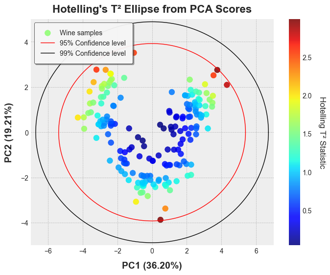
|
|
147
|
+
|
|
148
|
+
### Example 2: Grouped Confidence Ellipses
|
|
149
|
+
|
|
150
|
+
```python
|
|
151
|
+
wine_df['PC1'] = pca_scores[:, 0]
|
|
152
|
+
wine_df['PC2'] = pca_scores[:, 1]
|
|
153
|
+
|
|
154
|
+
colors = ['red', 'blue', 'green']
|
|
155
|
+
cultivars = wine_df['Cultivar'].unique()
|
|
156
|
+
color_map = {cultivar: color for cultivar, color in zip(cultivars, colors)}
|
|
157
|
+
point_colors = wine_df['Cultivar'].map(color_map)
|
|
158
|
+
|
|
159
|
+
# Plott PCA scores with confidence ellipses for each cultivar
|
|
160
|
+
plt.figure(figsize=(8, 6))
|
|
161
|
+
|
|
162
|
+
for i, cultivar in enumerate(cultivars):
|
|
163
|
+
mask = wine_df['Cultivar'] == cultivar
|
|
164
|
+
plt.scatter(
|
|
165
|
+
wine_df.loc[mask, 'PC1'], wine_df.loc[mask, 'PC2'], # type: ignore
|
|
166
|
+
c=colors[i], alpha=0.6, s=70, label=cultivar
|
|
167
|
+
)
|
|
168
|
+
|
|
169
|
+
ellipse_coords = confidence_ellipse(
|
|
170
|
+
data=wine_df,
|
|
171
|
+
x='PC1',
|
|
172
|
+
y='PC2',
|
|
173
|
+
group_by='Cultivar',
|
|
174
|
+
conf_level=0.95,
|
|
175
|
+
robust=True,
|
|
176
|
+
distribution='hotelling'
|
|
177
|
+
)
|
|
178
|
+
|
|
179
|
+
for i, cultivar in enumerate(cultivars):
|
|
180
|
+
ellipse_data = ellipse_coords[ellipse_coords['Cultivar'] == cultivar]
|
|
181
|
+
plt.plot(
|
|
182
|
+
ellipse_data['x'], ellipse_data['y'],
|
|
183
|
+
color=colors[i], linewidth=1, linestyle='-', label=f'{cultivar} (95% CI)'
|
|
184
|
+
)
|
|
185
|
+
|
|
186
|
+
plt.xlim(-1000, 1000)
|
|
187
|
+
plt.ylim(-50, 60)
|
|
188
|
+
plt.xlabel(f'PC1 ({explained_var[0]*100:.2f}%)', fontsize=14, labelpad=10, fontweight='bold')
|
|
189
|
+
plt.ylabel(f'PC2 ({explained_var[1]*100:.2f}%)', fontsize=14, labelpad=10, fontweight='bold')
|
|
190
|
+
plt.title("PCA Scores with Cultivar Group Confidence Ellipses", fontsize=16, pad=10, fontweight='bold')
|
|
191
|
+
plt.legend(
|
|
192
|
+
loc='upper left', fontsize=10, frameon=True, framealpha=0.9,
|
|
193
|
+
edgecolor='black', shadow=True, facecolor='white', borderpad=1
|
|
194
|
+
)
|
|
195
|
+
plt.show()
|
|
196
|
+
```
|
|
197
|
+
|
|
198
|
+
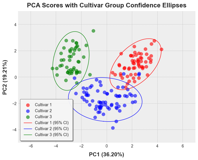
|
|
199
|
+
|
|
200
|
+
### Example 3: Grouped 3D Confidence Ellipsoids
|
|
201
|
+
|
|
202
|
+
```python
|
|
203
|
+
wine_df['PC1'] = pca_scores[:, 0]
|
|
204
|
+
wine_df['PC2'] = pca_scores[:, 1]
|
|
205
|
+
wine_df['PC3'] = pca_scores[:, 2]
|
|
206
|
+
|
|
207
|
+
colors = ['red', 'blue', 'green']
|
|
208
|
+
light_colors = ['lightcoral', 'lightblue', 'lightgreen']
|
|
209
|
+
cultivars = wine_df['Cultivar'].unique()
|
|
210
|
+
|
|
211
|
+
ellipse_coords = confidence_ellipse(
|
|
212
|
+
data=wine_df,
|
|
213
|
+
x='PC1',
|
|
214
|
+
y='PC2',
|
|
215
|
+
z='PC3',
|
|
216
|
+
group_by='Cultivar',
|
|
217
|
+
conf_level=0.95,
|
|
218
|
+
robust=True,
|
|
219
|
+
distribution='hotelling'
|
|
220
|
+
)
|
|
221
|
+
|
|
222
|
+
fig = plt.figure(figsize=(10, 6), facecolor='white')
|
|
223
|
+
ax = fig.add_subplot(111, projection='3d', facecolor='white')
|
|
224
|
+
|
|
225
|
+
for i, cultivar in enumerate(cultivars):
|
|
226
|
+
mask = wine_df['Cultivar'] == cultivar
|
|
227
|
+
ax.scatter(
|
|
228
|
+
wine_df.loc[mask, 'PC1'],
|
|
229
|
+
wine_df.loc[mask, 'PC2'],
|
|
230
|
+
wine_df.loc[mask, 'PC3'], # type: ignore
|
|
231
|
+
c=colors[i],
|
|
232
|
+
alpha=0.8,
|
|
233
|
+
s=50,
|
|
234
|
+
label=cultivar,
|
|
235
|
+
edgecolors='black',
|
|
236
|
+
linewidth=0.5
|
|
237
|
+
)
|
|
238
|
+
|
|
239
|
+
ellipse_data = ellipse_coords[ellipse_coords['Cultivar'] == cultivar]
|
|
240
|
+
n_points = int(np.sqrt(len(ellipse_data)))
|
|
241
|
+
|
|
242
|
+
x_2d = ellipse_data['x'].values.reshape(n_points, -1)
|
|
243
|
+
y_2d = ellipse_data['y'].values.reshape(n_points, -1)
|
|
244
|
+
z_2d = ellipse_data['z'].values.reshape(n_points, -1)
|
|
245
|
+
|
|
246
|
+
ax.plot_surface(
|
|
247
|
+
x_2d,
|
|
248
|
+
y_2d,
|
|
249
|
+
z_2d,
|
|
250
|
+
color=light_colors[i],
|
|
251
|
+
alpha=0.4,
|
|
252
|
+
linewidth=0,
|
|
253
|
+
antialiased=True
|
|
254
|
+
)
|
|
255
|
+
|
|
256
|
+
ax.set_xlabel(f'PC1 ({explained_var[0]*100:.2f}%)', fontsize=12, labelpad=5, fontweight='bold')
|
|
257
|
+
ax.set_ylabel(f'PC2 ({explained_var[1]*100:.2f}%)', fontsize=12, labelpad=5, fontweight='bold')
|
|
258
|
+
ax.set_zlabel(f'PC3 ({explained_var[2]*100:.2f}%)', fontsize=12, labelpad=1, fontweight='bold')
|
|
259
|
+
ax.set_title('3D PCA Scores with 95% Confidence Ellipsoids', fontsize=16, fontweight='bold')
|
|
260
|
+
ax.legend(
|
|
261
|
+
loc='upper right', fontsize=10, frameon=True, framealpha=0.9,
|
|
262
|
+
edgecolor='black', shadow=True, facecolor='white', borderpad=1
|
|
263
|
+
)
|
|
264
|
+
ax.grid(True, alpha=0.3, color='gray')
|
|
265
|
+
ax.view_init(elev=20, azim=65)
|
|
266
|
+
plt.tight_layout()
|
|
267
|
+
plt.show()
|
|
268
|
+
```
|
|
269
|
+
|
|
270
|
+
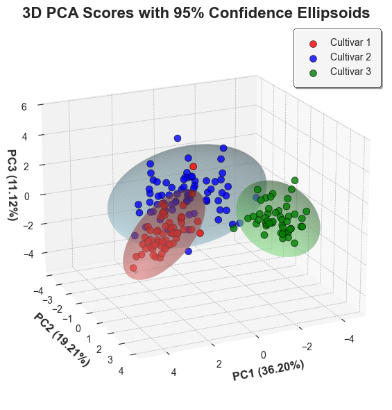
|
|
271
|
+
|
|
272
|
+
## Key Differences Between Functions
|
|
273
|
+
|
|
274
|
+
| Feature | `hotelling_parameters` | `hotelling_coordinates` | `confidence_ellipse` |
|
|
275
|
+
|---------|----------------|-----------------|---------------------|
|
|
276
|
+
| __Input__ | Component scores | Component scores | Raw data |
|
|
277
|
+
| __Purpose__ | T² statistics | Plot coordinates | Plot coordinates |
|
|
278
|
+
| __Grouping__ | -- | -- | Yes |
|
|
279
|
+
| __Robust__ | -- | -- | Yes |
|
|
280
|
+
| __2D/3D__ | 2D only for ellipse params | Both | Both |
|
|
281
|
+
| __Distribution__ | Hotelling only | Hotelling only | Normal or Hotelling |
|
|
282
|
+
| __Use Case__ | Outlier detection, QC | Visualizing PCA | Exploratory data analysis |
|
|
283
|
+
|
|
284
|
+
## When to Use Each Function
|
|
285
|
+
|
|
286
|
+
### Use `hotelling_parameters` when:
|
|
287
|
+
|
|
288
|
+
- You need T² statistics for outlier detection
|
|
289
|
+
- You want confidence cutoff values
|
|
290
|
+
- You're performing quality control or process monitoring
|
|
291
|
+
- You need ellipse parameters (semi-axes lengths)
|
|
292
|
+
|
|
293
|
+
### Use `hotelling_coordinates` when:
|
|
294
|
+
|
|
295
|
+
- You have PCA/PLS component scores
|
|
296
|
+
- You want to visualize confidence regions on score plots
|
|
297
|
+
- You need precise control over which components to plot
|
|
298
|
+
- You're creating publication-quality figures from multivariate models
|
|
299
|
+
|
|
300
|
+
### Use `confidence_ellipse` when:
|
|
301
|
+
|
|
302
|
+
- You're working with raw data (not scores)
|
|
303
|
+
- You need to compare multiple groups
|
|
304
|
+
- You want robust estimation for outlier-resistant analysis
|
|
305
|
+
- You need flexibility in distribution choice (normal vs Hotelling)
|
|
306
|
+
|
|
307
|
+
## References
|
|
308
|
+
|
|
309
|
+
1. Hotelling, H. (1931). The generalization of Student's ratio. *Annals of Mathematical Statistics*, 2(3), 360-378.
|
|
310
|
+
2. Brereton, R. G. (2016). Hotelling's T-squared distribution, its relationship to the F distribution and its use in multivariate space. *Journal of Chemometrics*, 30(1), 18-21.
|
|
311
|
+
3. Raymaekers, J., & Rousseeuw, P. J. (2019). Fast robust correlation for high dimensional data. *Technometrics*, 63(2), 184-198.
|
|
312
|
+
4. Jackson, J. E. (1991). *A User's Guide to Principal Components*. Wiley.
|
|
313
|
+
|
|
@@ -0,0 +1,8 @@
|
|
|
1
|
+
pyEllipse/__init__.py,sha256=e8UsmSroKa_4DUI65geZqkqkACibcE91yuANBwbfp54,1214
|
|
2
|
+
pyEllipse/confidence_ellipse.py,sha256=jPWGWN9WHvB6GzA7K6x3lJrRk8CNOMIkE_2QWTH7yRM,8700
|
|
3
|
+
pyEllipse/hotelling_coordinates.py,sha256=7nBtc9KHHLCsPgswWsBj2F7iNJKxgkGQOGVLOAspTwE,5162
|
|
4
|
+
pyEllipse/hotelling_parameters.py,sha256=7Xp49JWiaCJETgBE1ZDMWeJBV5Qr9dTqd35S6gVFKZg,8211
|
|
5
|
+
pyellipse-0.1.2.dist-info/METADATA,sha256=X9RWd-WO6POieGkNXxEe2nakdrfJo1xmcBFFvzAQmMY,11601
|
|
6
|
+
pyellipse-0.1.2.dist-info/WHEEL,sha256=M5asmiAlL6HEcOq52Yi5mmk9KmTVjY2RDPtO4p9DMrc,88
|
|
7
|
+
pyellipse-0.1.2.dist-info/licenses/LICENSE,sha256=aymc_9IU1zNJ7d2BKxzdgscT-atdAp7farpWhrGnXQ8,1078
|
|
8
|
+
pyellipse-0.1.2.dist-info/RECORD,,
|
|
@@ -0,0 +1,21 @@
|
|
|
1
|
+
MIT License
|
|
2
|
+
|
|
3
|
+
Copyright (c) 2025 Christian L. Goueguel
|
|
4
|
+
|
|
5
|
+
Permission is hereby granted, free of charge, to any person obtaining a copy
|
|
6
|
+
of this software and associated documentation files (the "Software"), to deal
|
|
7
|
+
in the Software without restriction, including without limitation the rights
|
|
8
|
+
to use, copy, modify, merge, publish, distribute, sublicense, and/or sell
|
|
9
|
+
copies of the Software, and to permit persons to whom the Software is
|
|
10
|
+
furnished to do so, subject to the following conditions:
|
|
11
|
+
|
|
12
|
+
The above copyright notice and this permission notice shall be included in all
|
|
13
|
+
copies or substantial portions of the Software.
|
|
14
|
+
|
|
15
|
+
THE SOFTWARE IS PROVIDED "AS IS", WITHOUT WARRANTY OF ANY KIND, EXPRESS OR
|
|
16
|
+
IMPLIED, INCLUDING BUT NOT LIMITED TO THE WARRANTIES OF MERCHANTABILITY,
|
|
17
|
+
FITNESS FOR A PARTICULAR PURPOSE AND NONINFRINGEMENT. IN NO EVENT SHALL THE
|
|
18
|
+
AUTHORS OR COPYRIGHT HOLDERS BE LIABLE FOR ANY CLAIM, DAMAGES OR OTHER
|
|
19
|
+
LIABILITY, WHETHER IN AN ACTION OF CONTRACT, TORT OR OTHERWISE, ARISING FROM,
|
|
20
|
+
OUT OF OR IN CONNECTION WITH THE SOFTWARE OR THE USE OR OTHER DEALINGS IN THE
|
|
21
|
+
SOFTWARE.
|