pixelplotlib 0.1.0__py3-none-any.whl
This diff represents the content of publicly available package versions that have been released to one of the supported registries. The information contained in this diff is provided for informational purposes only and reflects changes between package versions as they appear in their respective public registries.
- pixelplotlib/__init__.py +41 -0
- pixelplotlib/animation.py +73 -0
- pixelplotlib/artists.py +1313 -0
- pixelplotlib/axes.py +1123 -0
- pixelplotlib/canvas.py +369 -0
- pixelplotlib/colormaps.py +163 -0
- pixelplotlib/colors.py +143 -0
- pixelplotlib/dither.py +89 -0
- pixelplotlib/figure.py +259 -0
- pixelplotlib/fonts.py +358 -0
- pixelplotlib/markers.py +53 -0
- pixelplotlib/palettes.py +62 -0
- pixelplotlib/pyplot.py +106 -0
- pixelplotlib/rich.py +139 -0
- pixelplotlib/sixel.py +147 -0
- pixelplotlib/styles.py +347 -0
- pixelplotlib/textual.py +77 -0
- pixelplotlib/ticks.py +90 -0
- pixelplotlib-0.1.0.dist-info/METADATA +608 -0
- pixelplotlib-0.1.0.dist-info/RECORD +22 -0
- pixelplotlib-0.1.0.dist-info/WHEEL +4 -0
- pixelplotlib-0.1.0.dist-info/licenses/LICENSE +18 -0
|
@@ -0,0 +1,608 @@
|
|
|
1
|
+
Metadata-Version: 2.5
|
|
2
|
+
Name: pixelplotlib
|
|
3
|
+
Version: 0.1.0
|
|
4
|
+
Summary: Scientific plotting with 8-bit and 16-bit pixel-art graphics
|
|
5
|
+
Project-URL: Homepage, https://github.com/ap--/pixelplotlib
|
|
6
|
+
Project-URL: Source, https://github.com/ap--/pixelplotlib
|
|
7
|
+
Project-URL: Issues, https://github.com/ap--/pixelplotlib/issues
|
|
8
|
+
Project-URL: Changelog, https://github.com/ap--/pixelplotlib/releases
|
|
9
|
+
Author-email: Andreas Poehlmann <andreas@poehlmann.io>
|
|
10
|
+
Maintainer-email: Andreas Poehlmann <andreas@poehlmann.io>
|
|
11
|
+
License-Expression: MIT
|
|
12
|
+
License-File: LICENSE
|
|
13
|
+
Keywords: 16-bit,8-bit,pixel-art,plotting,retro,visualization
|
|
14
|
+
Classifier: Development Status :: 3 - Alpha
|
|
15
|
+
Classifier: Intended Audience :: Developers
|
|
16
|
+
Classifier: Intended Audience :: Science/Research
|
|
17
|
+
Classifier: Operating System :: OS Independent
|
|
18
|
+
Classifier: Programming Language :: Python :: 3
|
|
19
|
+
Classifier: Programming Language :: Python :: 3 :: Only
|
|
20
|
+
Classifier: Programming Language :: Python :: 3.11
|
|
21
|
+
Classifier: Programming Language :: Python :: 3.12
|
|
22
|
+
Classifier: Programming Language :: Python :: 3.13
|
|
23
|
+
Classifier: Programming Language :: Python :: 3.14
|
|
24
|
+
Classifier: Programming Language :: Python :: 3.15
|
|
25
|
+
Classifier: Topic :: Multimedia :: Graphics
|
|
26
|
+
Classifier: Topic :: Scientific/Engineering :: Visualization
|
|
27
|
+
Requires-Python: >=3.11
|
|
28
|
+
Requires-Dist: numpy>=1.23.2
|
|
29
|
+
Requires-Dist: pillow>=9.2
|
|
30
|
+
Provides-Extra: rich
|
|
31
|
+
Requires-Dist: rich>=12; extra == 'rich'
|
|
32
|
+
Provides-Extra: textual
|
|
33
|
+
Requires-Dist: textual>=0.86; extra == 'textual'
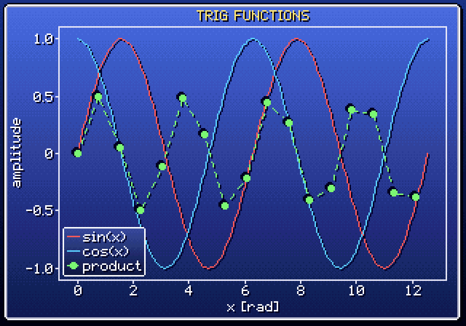
|
|
34
|
+
Description-Content-Type: text/markdown
|
|
35
|
+
|
|
36
|
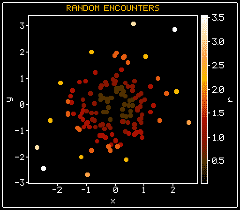
+
# pixelplotlib
|
|
37
|
+
|
|
38
|
+
**Scientific plots as 8-bit and 16-bit pixel art.**
|
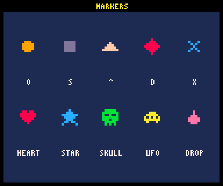
|
39
|
+
|
|
40
|
+
pixelplotlib is a small plotting library with a matplotlib-like API. Every figure is
|
|
41
|
+
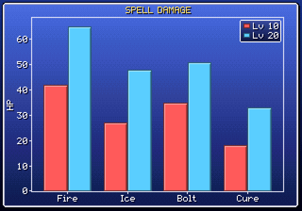
rendered on a low-resolution canvas with bitmap fonts, palettes from retro consoles,
|
|
42
|
+
ordered dithering and sprite markers, then upscaled with crisp nearest-neighbour pixels.
|
|
43
|
+
It depends only on [NumPy](https://numpy.org) and [Pillow](https://python-pillow.org).
|
|
44
|
+
|
|
45
|
+
|
|
46
|
+
|
|
47
|
+
## Features
|
|
48
|
+
|
|
49
|
+
- **Familiar API**: `fig, ax = ppl.subplots()`, `ax.plot(...)`, `ax.set(...)`, `fig.save(...)`,
|
|
50
|
+
plus a pyplot-style state machine (`ppl.plot`, `ppl.show`, ...).
|
|
51
|
+
- **Many plot types**: line, step, scatter, bar/barh, histograms (1-D and 2-D), fill_between,
|
|
52
|
+
error bars, stem, imshow, pcolormesh, contour/contourf, quiver, pie, box, violin,
|
|
53
|
+
annotations, reference lines/spans, log scales, colorbars, legends and subplot grids.
|
|
54
|
+
- **Retro styles**: `8bit` (NES), `16bit` (SNES-style 5-bit colour), `gameboy`, `pico8`,
|
|
55
|
+
`c64`, `cga` and `1bit`, each with its own resolution, palette, fonts and decorations.
|
|
56
|
+
- **Pixel-art rendering**: bitmap fonts, Bayer dithering for gradients and transparency,
|
|
57
|
+
palette-snapped colormaps, sprite markers (hearts, stars, skulls, UFOs, ...).
|
|
58
|
+
- **Output**: PNG (or any Pillow format) at integer scale, optional CRT scanlines, animated
|
|
59
|
+
GIFs, sixel graphics for plotting straight into the terminal, and
|
|
60
|
+
[Rich](https://github.com/Textualize/rich) / [Textual](https://github.com/Textualize/textual)
|
|
61
|
+
integration for terminal apps.
|
|
62
|
+
|
|
63
|
+
## Installation
|
|
64
|
+
|
|
65
|
+
pixelplotlib is available on [PyPI](https://pypi.org/project/pixelplotlib/). Add it to your
|
|
66
|
+
project with [uv](https://docs.astral.sh/uv/):
|
|
67
|
+
|
|
68
|
+
```bash
|
|
69
|
+
uv add pixelplotlib
|
|
70
|
+
```
|
|
71
|
+
|
|
72
|
+
or install it into the current environment with `uv pip install pixelplotlib` (or `pip install pixelplotlib`).
|
|
73
|
+
To try the latest development version use `uv add git+https://github.com/ap--/pixelplotlib`.
|
|
74
|
+
Python 3.11 or newer is required.
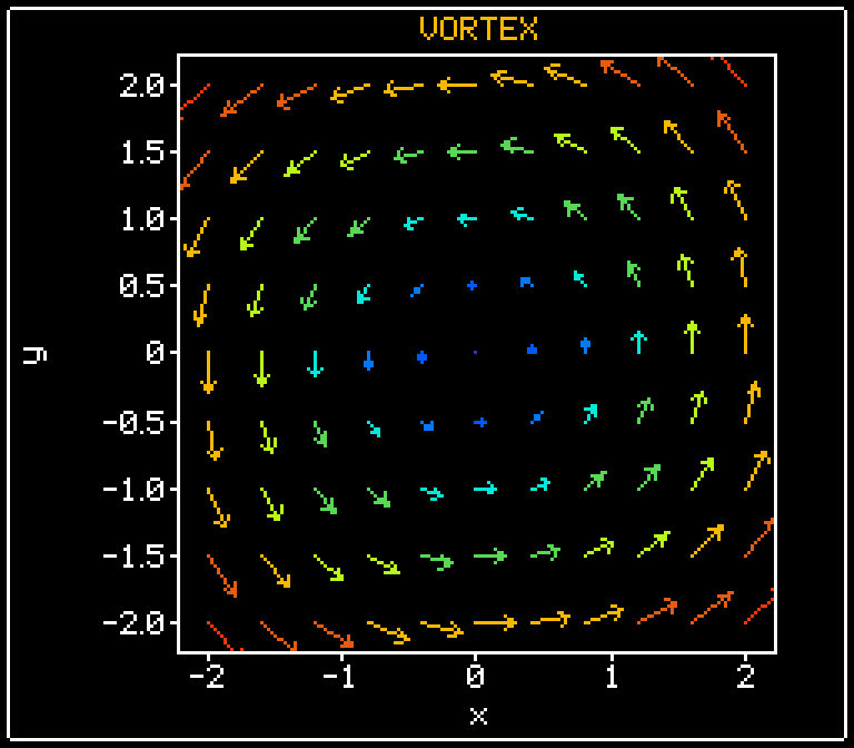
|
|
75
|
+
|
|
76
|
+
## Quick start
|
|
77
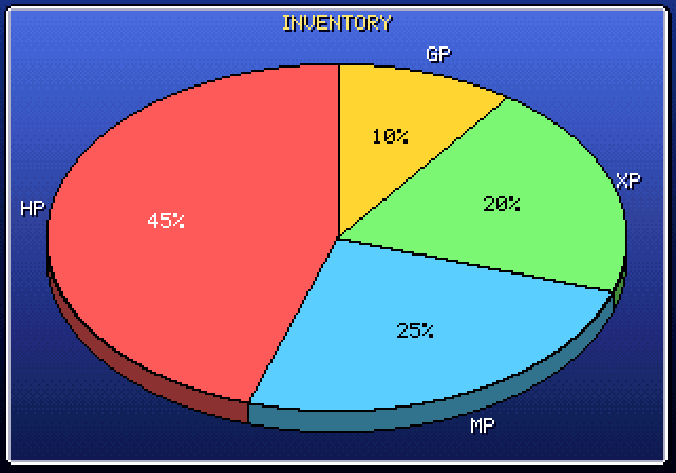
|
+
|
|
78
|
+
```python
|
|
79
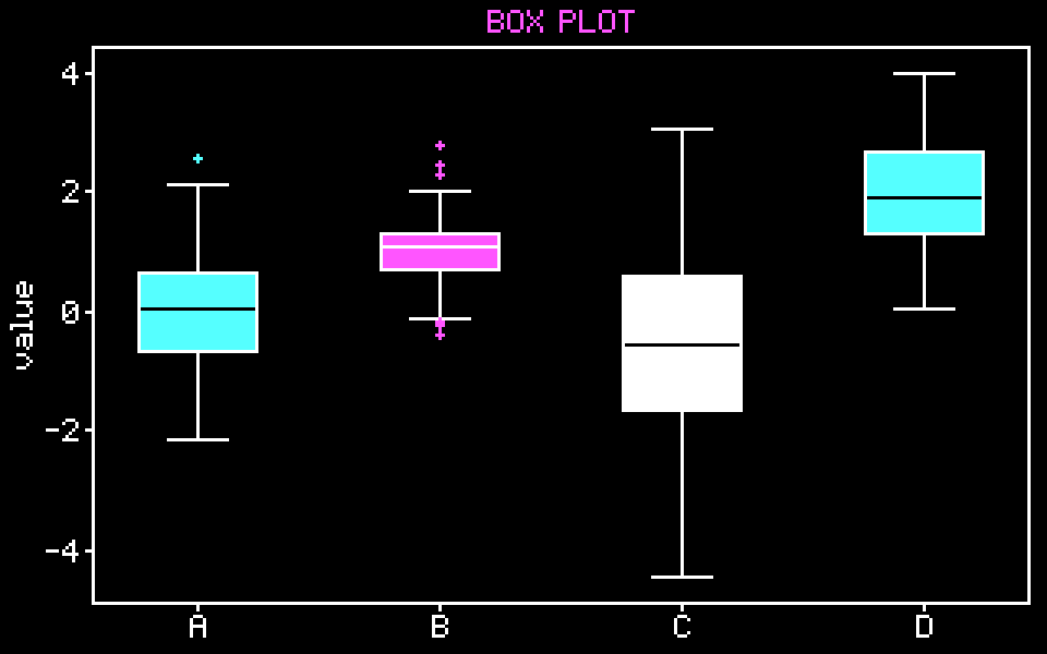
|
+
import numpy as np
|
|
80
|
+
import pixelplotlib as ppl
|
|
81
|
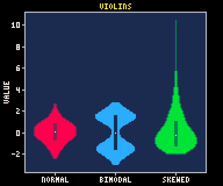
+
|
|
82
|
+
x = np.linspace(0, 10, 200)
|
|
83
|
+
fig, ax = ppl.subplots(style="16bit")
|
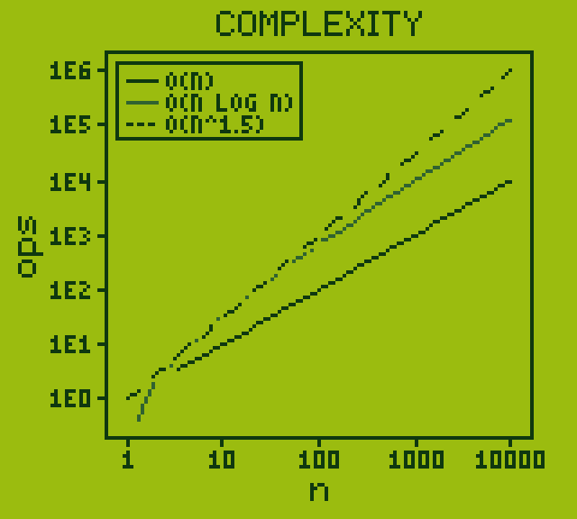
|
84
|
+
ax.plot(x, np.sin(x), label="sin")
|
|
85
|
+
ax.plot(x, np.cos(x), label="cos")
|
|
86
|
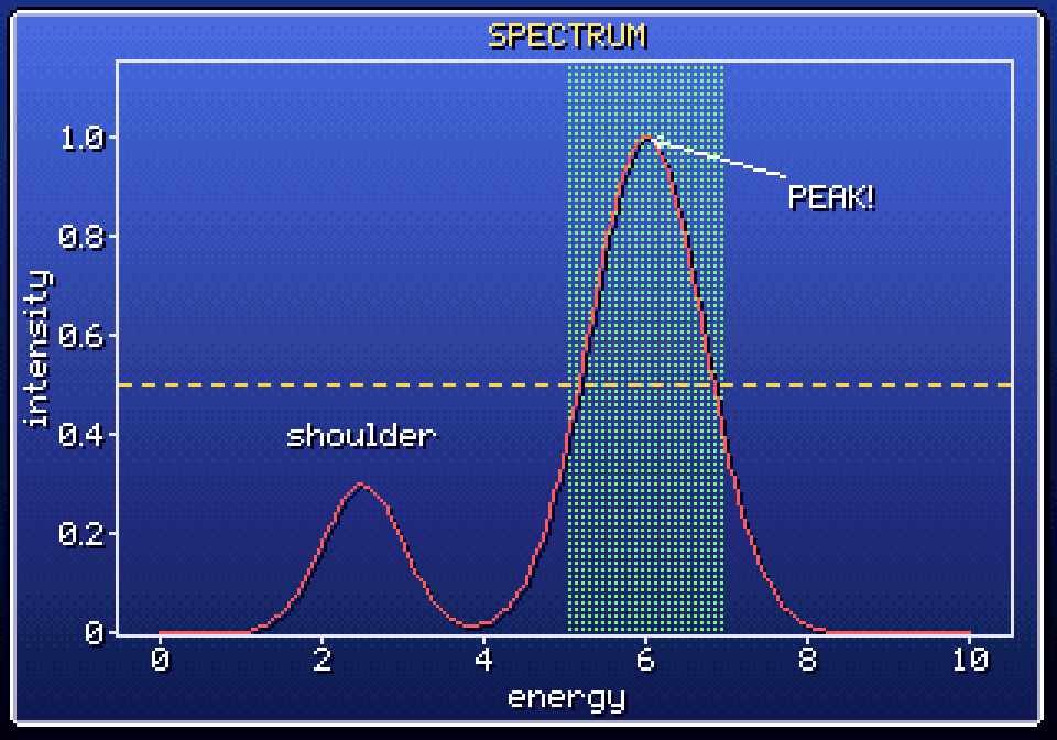
+
ax.set(title="HELLO WAVES", xlabel="t", ylabel="A")
|
|
87
|
+
ax.legend()
|
|
88
|
+
fig.save("waves.png") # upscaled by the style's default scale
|
|
89
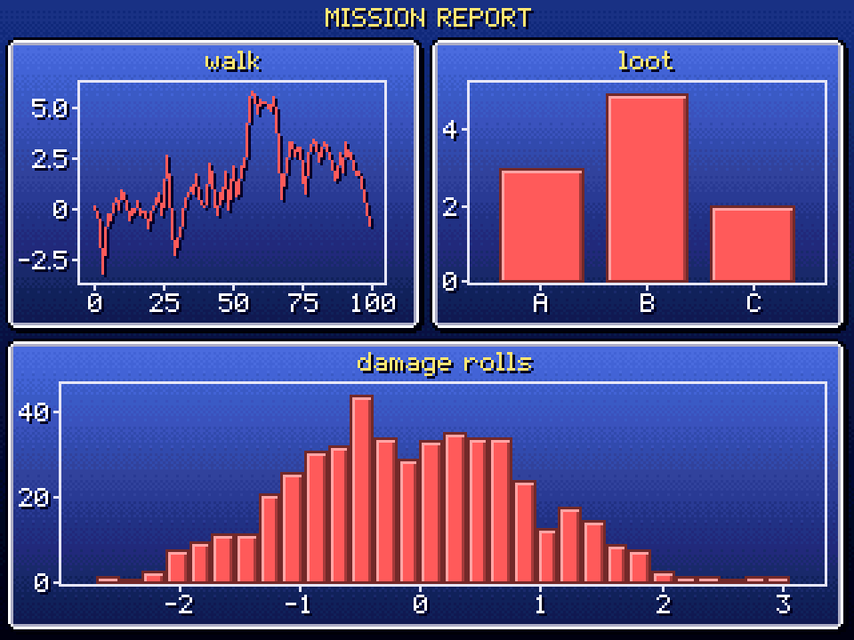
|
+
fig.save("waves_crt.png", scale=4, scanlines=True)
|
|
90
|
+
```
|
|
91
|
+
|
|
92
|
+
The pyplot-style interface works too:
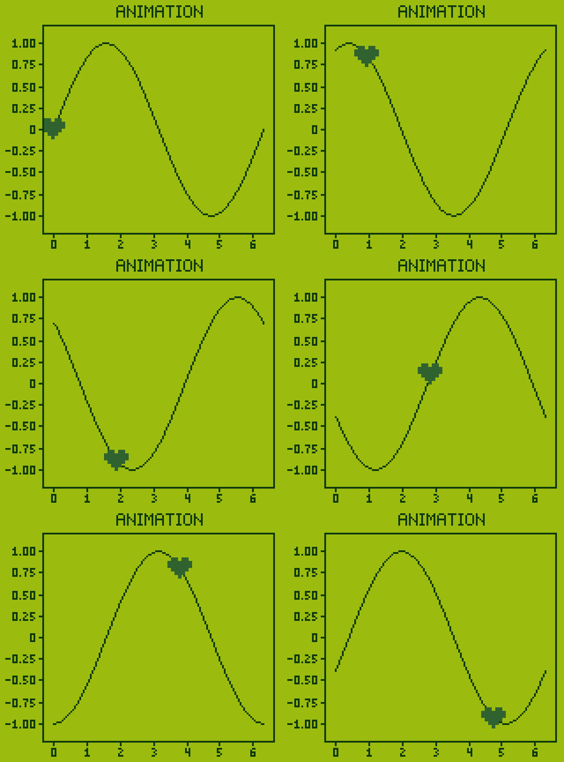
|
|
93
|
+
|
|
94
|
+
```python
|
|
95
|
+
import pixelplotlib.pyplot as plt # or: import pixelplotlib as plt
|
|
96
|
+
|
|
97
|
+
plt.figure(style="gameboy")
|
|
98
|
+
plt.plot([1, 3, 2, 4])
|
|
99
|
+
plt.title("GB")
|
|
100
|
+
plt.savefig("gb.png")
|
|
101
|
+
plt.show() # inline in Jupyter, else the system image viewer
|
|
102
|
+
```
|
|
103
|
+
|
|
104
|
+
Figures can also be returned as data: `fig.to_array()` gives the native-resolution RGB
|
|
105
|
+
array and `fig.to_image(scale=...)` a `PIL.Image`.
|
|
106
|
+
|
|
107
|
+
### Plotting in the terminal
|
|
108
|
+
|
|
109
|
+
In a terminal with [sixel](https://en.wikipedia.org/wiki/Sixel) graphics (xterm `-ti vt340`,
|
|
110
|
+
foot, WezTerm, mlterm, Konsole, iTerm2, Windows Terminal, tmux 3.4+, ...) figures are drawn
|
|
111
|
+
right in the terminal:
|
|
112
|
+
|
|
113
|
+
```python
|
|
114
|
+
fig.show(backend="sixel") # always write sixel to stdout
|
|
115
|
+
fig.show() # auto: Jupyter, else sixel if supported, else viewer
|
|
116
|
+
print(fig.to_sixel(scale=2)) # or grab the escape sequence yourself
|
|
117
|
+
```
|
|
118
|
+
|
|
119
|
+
`show()` detects sixel support by querying the terminal. Set `PIXELPLOTLIB_SIXEL=1` to force
|
|
120
|
+
sixel output (e.g. on Windows or through ssh/multiplexers that hide the reply) or
|
|
121
|
+
`PIXELPLOTLIB_SIXEL=0` to disable it.
|
|
122
|
+
|
|
123
|
+
### Rich and Textual
|
|
124
|
+
|
|
125
|
+
Figures also work in [Rich](https://github.com/Textualize/rich) and
|
|
126
|
+
[Textual](https://github.com/Textualize/textual), so they render in any terminal with
|
|
127
|
+
colour support (no sixel support needed). Each character cell shows two pixels as a
|
|
128
|
+
half block. Install the extras with `uv add "pixelplotlib[rich,textual]"`.
|
|
129
|
+
|
|
130
|
+
A `Figure` is a Rich renderable. Wrap it in `pixelplotlib.rich.Plot` to choose its size
|
|
131
|
+
in cells (`width=`, `height=`, or `expand=True` to fill the space):
|
|
132
|
+
|
|
133
|
+
```python
|
|
134
|
+
from rich import print
|
|
135
|
+
from rich.panel import Panel
|
|
136
|
+
from pixelplotlib.rich import Plot
|
|
137
|
+
|
|
138
|
+
print(fig) # native size, shrunk to fit the terminal width
|
|
139
|
+
print(Panel(Plot(fig, width=60), title="pixels"))
|
|
140
|
+
```
|
|
141
|
+
|
|
142
|
+
`pixelplotlib.textual.PixelPlot` is a Textual widget that fills its space (`1fr` by
|
|
143
|
+
default). Use `width: auto; height: auto` to show the figure at its native size instead:
|
|
144
|
+
|
|
145
|
+
```python
|
|
146
|
+
from textual.app import App
|
|
147
|
+
from pixelplotlib.textual import PixelPlot
|
|
148
|
+
|
|
149
|
+
class PlotApp(App):
|
|
150
|
+
def compose(self):
|
|
151
|
+
fig, ax = ppl.subplots(style="pico8")
|
|
152
|
+
ax.plot([1, 3, 2, 4])
|
|
153
|
+
yield PixelPlot(fig)
|
|
154
|
+
|
|
155
|
+
PlotApp().run()
|
|
156
|
+
```
|
|
157
|
+
|
|
158
|
+
Assign a new figure to `widget.figure` to replace the plot, or call `widget.refresh()`
|
|
159
|
+
after changing the current figure. Both integrations re-render the figure at the size
|
|
160
|
+
they draw it, so text and one-pixel lines stay sharp. `fig.to_array(size=(w, h))` gives
|
|
161
|
+
the same re-rendered pixels as an array. [`examples/textual_app.py`](https://github.com/ap--/pixelplotlib/blob/v0.1.0/examples/textual_app.py)
|
|
162
|
+
is a live dashboard: run it with `uv run --extra textual python examples/textual_app.py`.
|
|
163
|
+
|
|
164
|
+
## Styles
|
|
165
|
+
|
|
166
|
+
Pick a style per figure (`ppl.subplots(style="pico8")`), globally (`ppl.use("c64")`) or
|
|
167
|
+
temporarily (`with ppl.context("1bit"): ...`). The canvas size in the table is the
|
|
168
|
+
native resolution, which is upscaled when saving.
|
|
169
|
+
|
|
170
|
+
<!-- styles:start -->
|
|
171
|
+
<table>
|
|
172
|
+
<tr><td align="center"><img src="https://raw.githubusercontent.com/ap--/pixelplotlib/v0.1.0/docs/images/style_8bit.png" width="320"><br><code>8bit</code> (256x224)</td><td align="center"><img src="https://raw.githubusercontent.com/ap--/pixelplotlib/v0.1.0/docs/images/style_16bit.png" width="320"><br><code>16bit</code> (320x224)</td></tr>
|
|
173
|
+
<tr><td align="center"><img src="https://raw.githubusercontent.com/ap--/pixelplotlib/v0.1.0/docs/images/style_gameboy.png" width="320"><br><code>gameboy</code> (160x144)</td><td align="center"><img src="https://raw.githubusercontent.com/ap--/pixelplotlib/v0.1.0/docs/images/style_pico8.png" width="320"><br><code>pico8</code> (192x160)</td></tr>
|
|
174
|
+
<tr><td align="center"><img src="https://raw.githubusercontent.com/ap--/pixelplotlib/v0.1.0/docs/images/style_c64.png" width="320"><br><code>c64</code> (320x200)</td><td align="center"><img src="https://raw.githubusercontent.com/ap--/pixelplotlib/v0.1.0/docs/images/style_cga.png" width="320"><br><code>cga</code> (320x200)</td></tr>
|
|
175
|
+
<tr><td align="center"><img src="https://raw.githubusercontent.com/ap--/pixelplotlib/v0.1.0/docs/images/style_1bit.png" width="320"><br><code>1bit</code> (256x192)</td></tr>
|
|
176
|
+
</table>
|
|
177
|
+
|
|
178
|
+
<details><summary>Code for the style demo</summary>
|
|
179
|
+
|
|
180
|
+
```python
|
|
181
|
+
rng = np.random.default_rng(0)
|
|
182
|
+
x = np.linspace(0, 10, 100)
|
|
183
|
+
fig, (ax1, ax2) = ppl.subplots(1, 2, style="16bit")
|
|
184
|
+
ax1.fill_between(x, np.sin(x) - 0.4, np.sin(x) + 0.4)
|
|
185
|
+
ax1.plot(x, np.sin(x), label="sin")
|
|
186
|
+
ax1.plot(x, np.cos(x), label="cos")
|
|
187
|
+
ax1.set(title=style, xlabel="t")
|
|
188
|
+
ax2.hist(rng.normal(size=300), bins=8)
|
|
189
|
+
ax2.set(title="hist")
|
|
190
|
+
```
|
|
191
|
+
|
|
192
|
+
</details>
|
|
193
|
+
<!-- styles:end -->
|
|
194
|
+
|
|
195
|
+
### Custom styles
|
|
196
|
+
|
|
197
|
+
Styles are dataclasses. Derive a new one with `Style.replace` and register it:
|
|
198
|
+
|
|
199
|
+
```python
|
|
200
|
+
neon = ppl.get_style("16bit").replace(
|
|
201
|
+
name="neon",
|
|
202
|
+
background="#000000",
|
|
203
|
+
series=["#ff00ff", "#00ffff", "#ffff00"],
|
|
204
|
+
cmap="plasma",
|
|
205
|
+
)
|
|
206
|
+
ppl.register(neon)
|
|
207
|
+
fig, ax = ppl.subplots(style="neon")
|
|
208
|
+
```
|
|
209
|
+
|
|
210
|
+
Useful fields include `size`, `scale`, `palette` (snap every colour to a fixed palette),
|
|
211
|
+
`bits` (bits per colour channel), `font`/`tick_font`, `line_width`, `line_shadow`,
|
|
212
|
+
`line_halo`, `bar_shading`, `panel` and `dither`.
|
|
213
|
+
|
|
214
|
+
## Plot types
|
|
215
|
+
|
|
216
|
+
Every image below was produced by the code shown next to it
|
|
217
|
+
(see [`examples/gallery.py`](https://github.com/ap--/pixelplotlib/blob/v0.1.0/examples/gallery.py)).
|
|
218
|
+
|
|
219
|
+
<!-- gallery:start -->
|
|
220
|
+
### Line plot
|
|
221
|
+
|
|
222
|
+

|
|
223
|
+
|
|
224
|
+
```python
|
|
225
|
+
x = np.linspace(0, 4 * np.pi, 200)
|
|
226
|
+
fig, ax = ppl.subplots(style="16bit")
|
|
227
|
+
ax.plot(x, np.sin(x), label="sin(x)")
|
|
228
|
+
ax.plot(x, np.cos(x), label="cos(x)")
|
|
229
|
+
ax.plot(x[::12], np.sin(x[::12]) * np.cos(x[::12]), "o--", label="product")
|
|
230
|
+
ax.set(title="TRIG FUNCTIONS", xlabel="x [rad]", ylabel="amplitude")
|
|
231
|
+
ax.legend(loc="lower left")
|
|
232
|
+
fig.save("line_plot.png")
|
|
233
|
+
```
|
|
234
|
+
|
|
235
|
+
### Scatter plot
|
|
236
|
+
|
|
237
|
+
|
|
238
|
+
|
|
239
|
+
```python
|
|
240
|
+
rng = np.random.default_rng(1)
|
|
241
|
+
x, y = rng.normal(size=(2, 150))
|
|
242
|
+
fig, ax = ppl.subplots(style="8bit")
|
|
243
|
+
sc = ax.scatter(x, y, c=np.hypot(x, y), cmap="fire")
|
|
244
|
+
ax.set(title="RANDOM ENCOUNTERS", xlabel="x", ylabel="y")
|
|
245
|
+
ax.colorbar(sc, label="r")
|
|
246
|
+
fig.save("scatter_plot.png")
|
|
247
|
+
```
|
|
248
|
+
|
|
249
|
+
### Sprite markers
|
|
250
|
+
|
|
251
|
+
|
|
252
|
+
|
|
253
|
+
```python
|
|
254
|
+
fig, ax = ppl.subplots(style="pico8")
|
|
255
|
+
markers = ["heart", "star", "skull", "ufo", "drop", "o", "s", "^", "D", "x"]
|
|
256
|
+
for i, m in enumerate(markers):
|
|
257
|
+
ax.scatter([i % 5], [i // 5], marker=m, size=2, color=f"C{i}")
|
|
258
|
+
ax.text(i % 5, i // 5 - 0.45, m, ha="center", va="top")
|
|
259
|
+
ax.set(title="MARKERS", xlim=(-0.6, 4.6), ylim=(-0.9, 1.5))
|
|
260
|
+
ax.axis("off")
|
|
261
|
+
fig.save("sprite_markers.png")
|
|
262
|
+
```
|
|
263
|
+
|
|
264
|
+
### Bar chart
|
|
265
|
+
|
|
266
|
+
|
|
267
|
+
|
|
268
|
+
```python
|
|
269
|
+
labels = ["Fire", "Ice", "Bolt", "Cure"]
|
|
270
|
+
fig, ax = ppl.subplots(style="16bit")
|
|
271
|
+
x = np.arange(len(labels))
|
|
272
|
+
ax.bar(x - 0.2, [42, 27, 35, 18], width=0.4, label="Lv 10")
|
|
273
|
+
ax.bar(x + 0.2, [65, 48, 51, 33], width=0.4, label="Lv 20")
|
|
274
|
+
ax.set_xticks(x, labels)
|
|
275
|
+
ax.set(title="SPELL DAMAGE", ylabel="HP")
|
|
276
|
+
ax.legend(loc="upper right")
|
|
277
|
+
fig.save("bar_chart.png")
|
|
278
|
+
```
|
|
279
|
+
|
|
280
|
+
### Horizontal bars
|
|
281
|
+
|
|
282
|
+
|
|
283
|
+
|
|
284
|
+
```python
|
|
285
|
+
fig, ax = ppl.subplots(style="c64")
|
|
286
|
+
langs = ["BASIC", "C", "ASM", "PASCAL", "FORTH"]
|
|
287
|
+
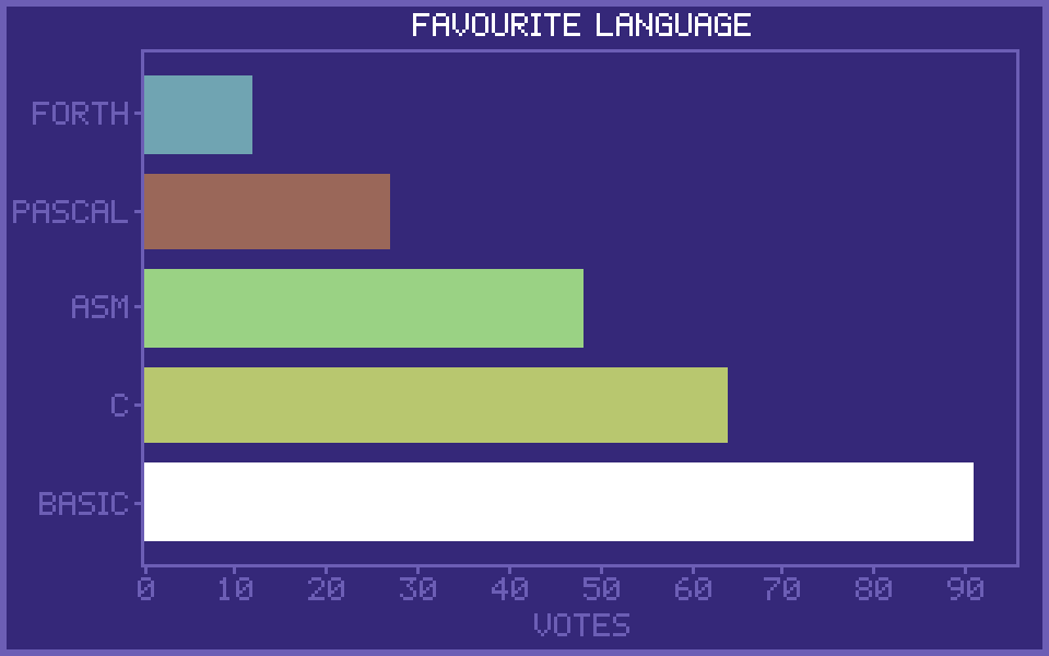
ax.barh(langs, [91, 64, 48, 27, 12], color=[f"C{i}" for i in range(5)])
|
|
288
|
+
ax.set(title="Favourite language", xlabel="votes")
|
|
289
|
+
fig.save("barh_chart.png")
|
|
290
|
+
```
|
|
291
|
+
|
|
292
|
+
### Histogram
|
|
293
|
+
|
|
294
|
+
|
|
295
|
+
|
|
296
|
+
```python
|
|
297
|
+
rng = np.random.default_rng(7)
|
|
298
|
+
fig, ax = ppl.subplots(style="gameboy")
|
|
299
|
+
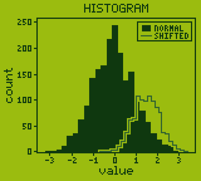
ax.hist(rng.normal(0, 1, 2000), bins=24, label="normal")
|
|
300
|
+
ax.hist(rng.normal(1.5, 0.6, 1000), bins=24, histtype="step", label="shifted")
|
|
301
|
+
ax.set(title="HISTOGRAM", xlabel="value", ylabel="count")
|
|
302
|
+
ax.legend()
|
|
303
|
+
fig.save("histogram.png")
|
|
304
|
+
```
|
|
305
|
+
|
|
306
|
+
### 2-D histogram
|
|
307
|
+
|
|
308
|
+
|
|
309
|
+
|
|
310
|
+
```python
|
|
311
|
+
rng = np.random.default_rng(3)
|
|
312
|
+
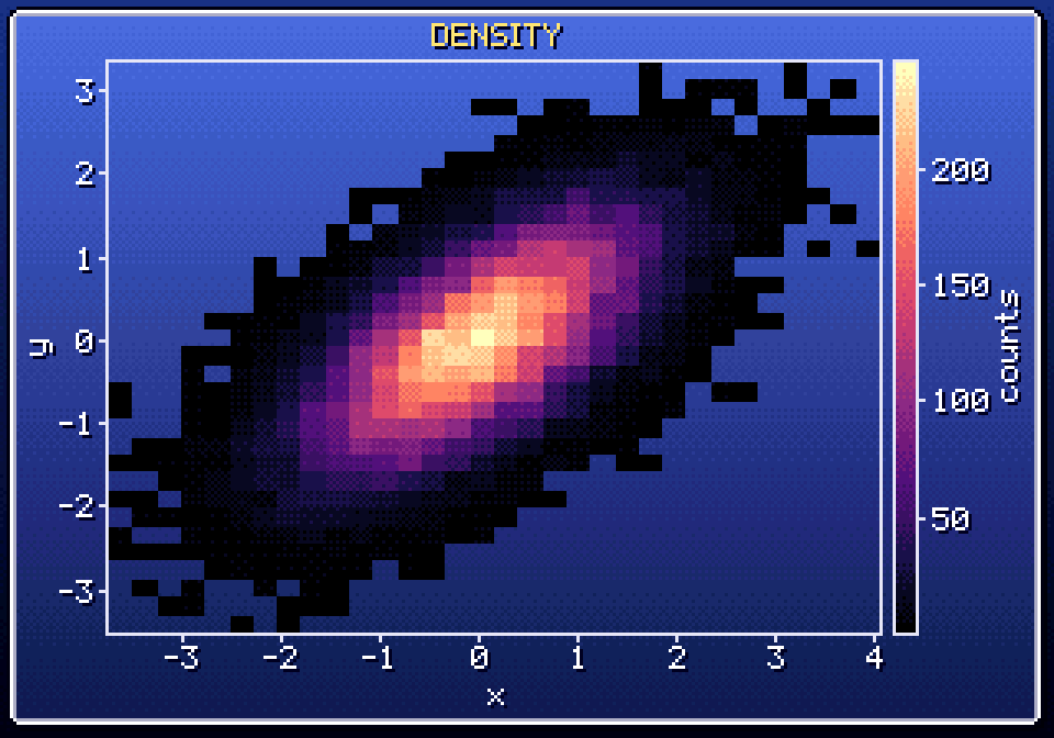
x = rng.normal(size=20000)
|
|
313
|
+
y = 0.6 * x + rng.normal(scale=0.7, size=20000)
|
|
314
|
+
fig, ax = ppl.subplots(style="16bit")
|
|
315
|
+
_, _, _, mesh = ax.hist2d(x, y, bins=32, cmap="magma")
|
|
316
|
+
ax.colorbar(mesh, label="counts")
|
|
317
|
+
ax.set(title="DENSITY", xlabel="x", ylabel="y")
|
|
318
|
+
fig.save("histogram_2d.png")
|
|
319
|
+
```
|
|
320
|
+
|
|
321
|
+
### Filled areas
|
|
322
|
+
|
|
323
|
+
|
|
324
|
+
|
|
325
|
+
```python
|
|
326
|
+
x = np.linspace(0, 10, 120)
|
|
327
|
+
y = np.sin(x) * np.exp(-x / 8)
|
|
328
|
+
fig, ax = ppl.subplots(style="1bit")
|
|
329
|
+
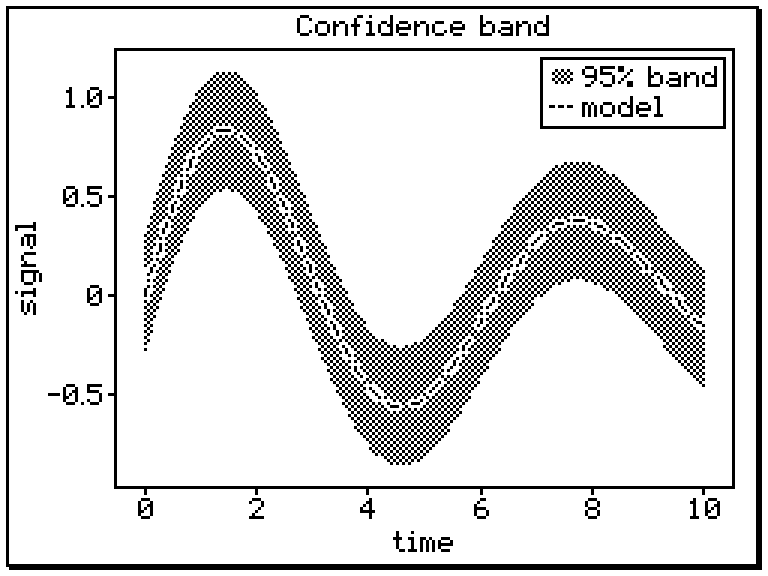
ax.fill_between(x, y - 0.3, y + 0.3, label="95% band")
|
|
330
|
+
ax.plot(x, y, label="model")
|
|
331
|
+
ax.set(title="Confidence band", xlabel="time", ylabel="signal")
|
|
332
|
+
ax.legend()
|
|
333
|
+
fig.save("fill_between.png")
|
|
334
|
+
```
|
|
335
|
+
|
|
336
|
+
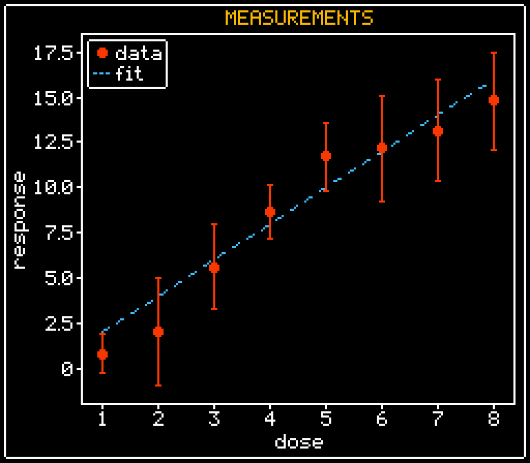
### Error bars
|
|
337
|
+
|
|
338
|
+
|
|
339
|
+
|
|
340
|
+
```python
|
|
341
|
+
rng = np.random.default_rng(5)
|
|
342
|
+
x = np.arange(1, 9)
|
|
343
|
+
y = 2.0 * x + rng.normal(0, 1.5, x.size)
|
|
344
|
+
fig, ax = ppl.subplots(style="8bit")
|
|
345
|
+
ax.errorbar(x, y, yerr=rng.uniform(1, 3, x.size), label="data")
|
|
346
|
+
ax.plot(x, 2.0 * x, "--", label="fit")
|
|
347
|
+
ax.set(title="MEASUREMENTS", xlabel="dose", ylabel="response")
|
|
348
|
+
ax.legend(loc="upper left")
|
|
349
|
+
fig.save("error_bars.png")
|
|
350
|
+
```
|
|
351
|
+
|
|
352
|
+
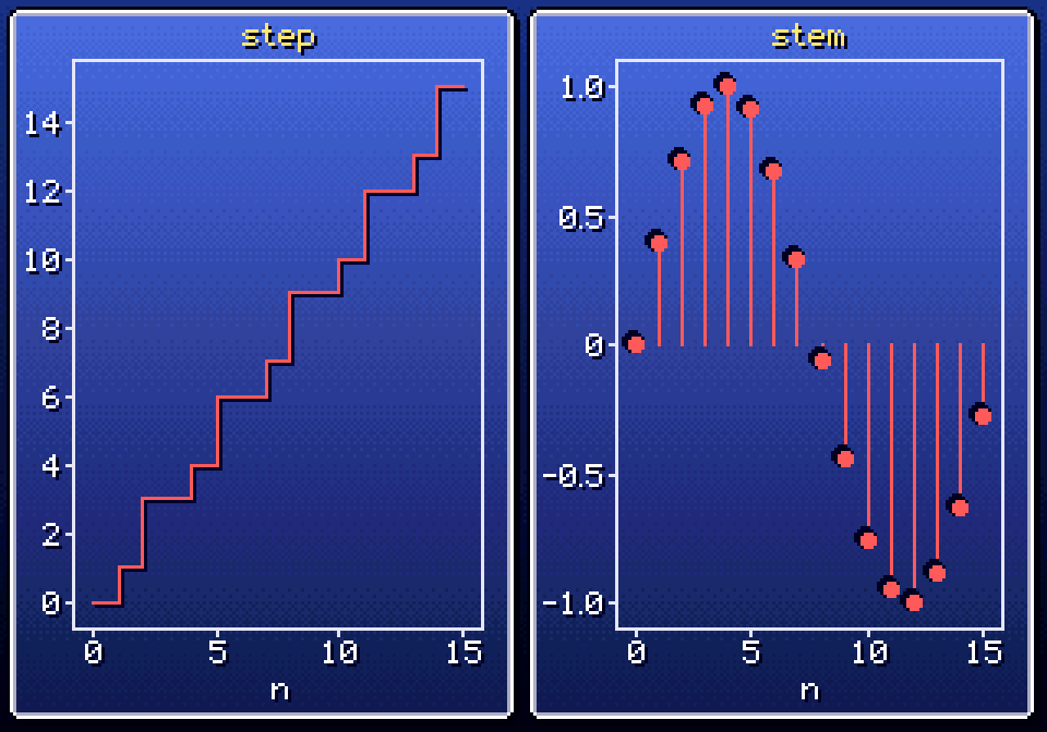
### Step and stem plots
|
|
353
|
+
|
|
354
|
+
|
|
355
|
+
|
|
356
|
+
```python
|
|
357
|
+
n = np.arange(16)
|
|
358
|
+
fig, (ax1, ax2) = ppl.subplots(1, 2, style="snes")
|
|
359
|
+
ax1.step(n, np.cumsum(n % 3), where="post")
|
|
360
|
+
ax1.set(title="step", xlabel="n")
|
|
361
|
+
ax2.stem(n, np.sin(n / 2.5))
|
|
362
|
+
ax2.set(title="stem", xlabel="n")
|
|
363
|
+
fig.save("step_and_stem.png")
|
|
364
|
+
```
|
|
365
|
+
|
|
366
|
+
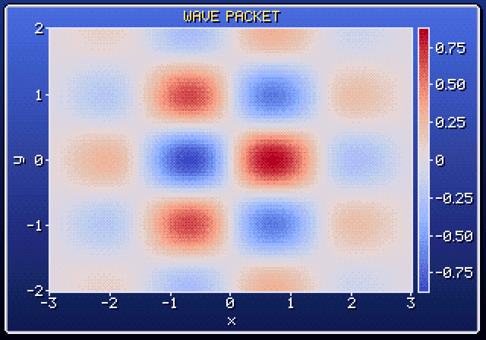
### Image / heatmap
|
|
367
|
+
|
|
368
|
+
|
|
369
|
+
|
|
370
|
+
```python
|
|
371
|
+
y, x = np.mgrid[-2:2:64j, -3:3:96j]
|
|
372
|
+
z = np.sin(x * 2) * np.cos(y * 3) * np.exp(-(x**2 + y**2) / 4)
|
|
373
|
+
fig, ax = ppl.subplots(style="16bit")
|
|
374
|
+
im = ax.imshow(z, cmap="coolwarm", extent=(-3, 3, -2, 2), origin="lower")
|
|
375
|
+
ax.colorbar(im)
|
|
376
|
+
ax.set(title="WAVE PACKET", xlabel="x", ylabel="y")
|
|
377
|
+
fig.save("heatmap.png")
|
|
378
|
+
```
|
|
379
|
+
|
|
380
|
+
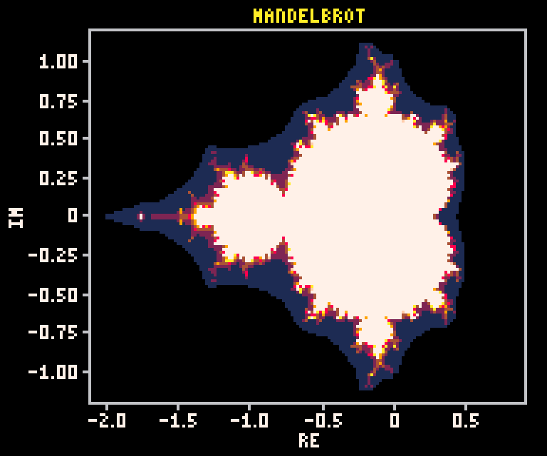
### Mandelbrot (imshow without dithering)
|
|
381
|
+
|
|
382
|
+
|
|
383
|
+
|
|
384
|
+
```python
|
|
385
|
+
y, x = np.mgrid[-1.2:1.2:150j, -2.1:0.9:200j]
|
|
386
|
+
c = x + 1j * y
|
|
387
|
+
z = np.zeros_like(c)
|
|
388
|
+
count = np.zeros(c.shape)
|
|
389
|
+
for _ in range(40):
|
|
390
|
+
z = np.where(np.abs(z) < 4, z * z + c, z)
|
|
391
|
+
count += np.abs(z) < 4
|
|
392
|
+
fig, ax = ppl.subplots(style="pico8")
|
|
393
|
+
ax.imshow(count, cmap="pico", dither=False, origin="lower", extent=(-2.1, 0.9, -1.2, 1.2))
|
|
394
|
+
ax.set(title="MANDELBROT", xlabel="Re", ylabel="Im")
|
|
395
|
+
fig.save("mandelbrot.png")
|
|
396
|
+
```
|
|
397
|
+
|
|
398
|
+
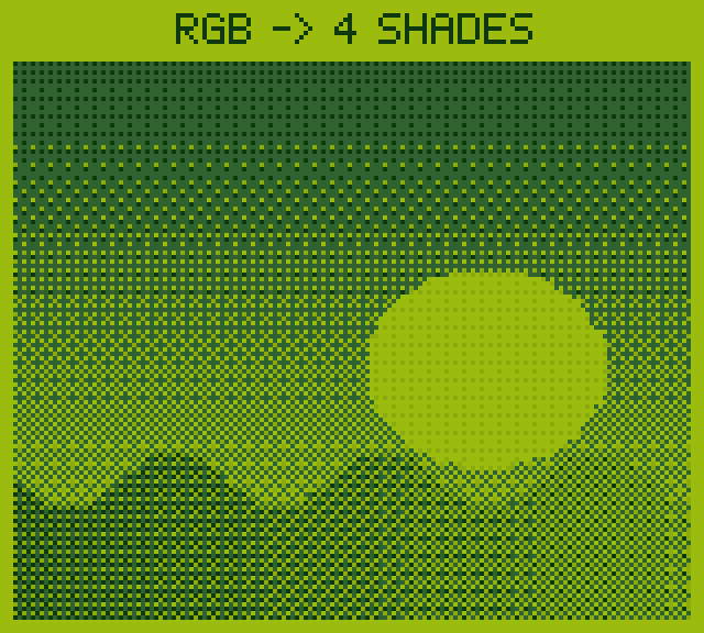
### Pixelated RGB image
|
|
399
|
+
|
|
400
|
+
|
|
401
|
+
|
|
402
|
+
```python
|
|
403
|
+
y, x = np.mgrid[0:1:96j, 0:1:128j]
|
|
404
|
+
sky = np.stack([40 + 120 * y, 60 + 140 * y, 200 - 60 * y], axis=-1)
|
|
405
|
+
sun = np.hypot(x - 0.7, y - 0.55) < 0.18
|
|
406
|
+
sky[sun] = (255, 200, 60)
|
|
407
|
+
ground = y > 0.75 + 0.05 * np.sin(x * 20)
|
|
408
|
+
sky[ground] = np.stack([30 + 20 * x, 120 + 60 * x, 40 + 0 * x], axis=-1)[ground]
|
|
409
|
+
fig, ax = ppl.subplots(style="gameboy")
|
|
410
|
+
ax.imshow(sky.astype(np.uint8))
|
|
411
|
+
ax.set(title="RGB -> 4 SHADES")
|
|
412
|
+
ax.axis("off")
|
|
413
|
+
fig.save("rgb_image.png")
|
|
414
|
+
```
|
|
415
|
+
|
|
416
|
+
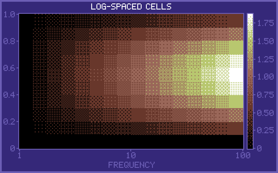
### Pcolormesh (irregular grid)
|
|
417
|
+
|
|
418
|
+
|
|
419
|
+
|
|
420
|
+
```python
|
|
421
|
+
xe = np.geomspace(1, 100, 17)
|
|
422
|
+
ye = np.linspace(0, 1, 11)
|
|
423
|
+
c = np.log10(xe[:-1])[None, :] * np.sin(np.pi * ye[:-1])[:, None]
|
|
424
|
+
fig, ax = ppl.subplots(style="c64")
|
|
425
|
+
mesh = ax.pcolormesh(xe, ye, c, cmap="fire")
|
|
426
|
+
ax.set_xscale("log")
|
|
427
|
+
ax.colorbar(mesh)
|
|
428
|
+
ax.set(title="Log-spaced cells", xlabel="frequency")
|
|
429
|
+
fig.save("pcolormesh.png")
|
|
430
|
+
```
|
|
431
|
+
|
|
432
|
+
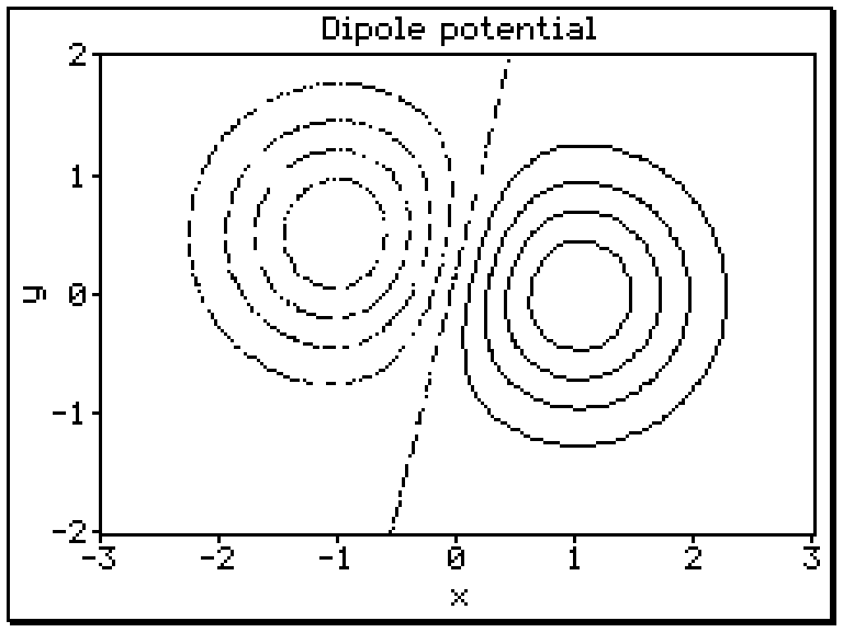
### Contour lines
|
|
433
|
+
|
|
434
|
+
|
|
435
|
+
|
|
436
|
+
```python
|
|
437
|
+
y, x = np.mgrid[-2:2:80j, -3:3:120j]
|
|
438
|
+
z = np.exp(-((x - 1) ** 2 + y**2)) - np.exp(-((x + 1) ** 2 + (y - 0.5) ** 2))
|
|
439
|
+
fig, ax = ppl.subplots(style="1bit")
|
|
440
|
+
ax.contour(x, y, z, levels=10, colors="fg")
|
|
441
|
+
ax.set(title="Dipole potential", xlabel="x", ylabel="y")
|
|
442
|
+
fig.save("contour_lines.png")
|
|
443
|
+
```
|
|
444
|
+
|
|
445
|
+
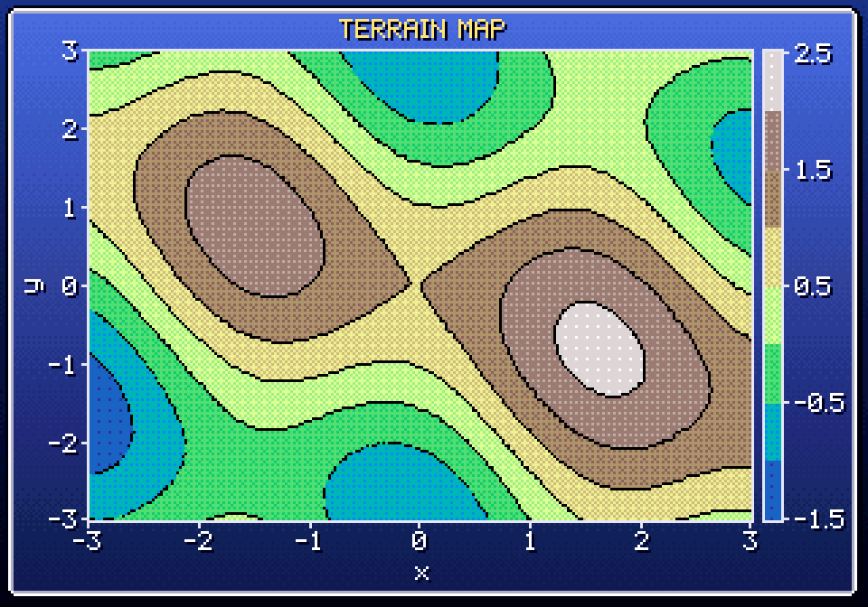
### Filled contours
|
|
446
|
+
|
|
447
|
+
|
|
448
|
+
|
|
449
|
+
```python
|
|
450
|
+
y, x = np.mgrid[-3:3:90j, -3:3:120j]
|
|
451
|
+
z = np.sin(x) ** 2 + np.cos(y + x / 2) + 0.1 * x
|
|
452
|
+
fig, ax = ppl.subplots(style="16bit")
|
|
453
|
+
cs = ax.contourf(x, y, z, levels=8, cmap="terrain")
|
|
454
|
+
ax.contour(x, y, z, levels=8, colors="#000000")
|
|
455
|
+
ax.colorbar(cs)
|
|
456
|
+
ax.set(title="TERRAIN MAP", xlabel="x", ylabel="y")
|
|
457
|
+
fig.save("filled_contours.png")
|
|
458
|
+
```
|
|
459
|
+
|
|
460
|
+
### Vector field (quiver)
|
|
461
|
+
|
|
462
|
+
|
|
463
|
+
|
|
464
|
+
```python
|
|
465
|
+
y, x = np.mgrid[-2:2:9j, -2:2:11j]
|
|
466
|
+
u, v = -y, x
|
|
467
|
+
fig, ax = ppl.subplots(style="8bit")
|
|
468
|
+
ax.quiver(x, y, u, v, C=np.hypot(u, v), cmap="rainbow")
|
|
469
|
+
ax.set(title="VORTEX", xlabel="x", ylabel="y")
|
|
470
|
+
ax.set_aspect("equal")
|
|
471
|
+
fig.save("quiver.png")
|
|
472
|
+
```
|
|
473
|
+
|
|
474
|
+
### Pie chart
|
|
475
|
+
|
|
476
|
+
|
|
477
|
+
|
|
478
|
+
```python
|
|
479
|
+
fig, ax = ppl.subplots(style="16bit")
|
|
480
|
+
ax.pie([45, 25, 20, 10], labels=["HP", "MP", "XP", "GP"], autopct="%d%%")
|
|
481
|
+
ax.set_title("INVENTORY")
|
|
482
|
+
fig.save("pie_chart.png")
|
|
483
|
+
```
|
|
484
|
+
|
|
485
|
+
### Box plot
|
|
486
|
+
|
|
487
|
+
|
|
488
|
+
|
|
489
|
+
```python
|
|
490
|
+
rng = np.random.default_rng(11)
|
|
491
|
+
data = [rng.normal(mu, sd, 200) for mu, sd in [(0, 1), (1, 0.5), (-0.5, 1.5), (2, 0.8)]]
|
|
492
|
+
fig, ax = ppl.subplots(style="cga")
|
|
493
|
+
ax.boxplot(data, labels=["A", "B", "C", "D"])
|
|
494
|
+
ax.set(title="BOX PLOT", ylabel="value")
|
|
495
|
+
fig.save("box_plot.png")
|
|
496
|
+
```
|
|
497
|
+
|
|
498
|
+
### Violin plot
|
|
499
|
+
|
|
500
|
+
|
|
501
|
+
|
|
502
|
+
```python
|
|
503
|
+
rng = np.random.default_rng(12)
|
|
504
|
+
data = [rng.normal(0, 1, 300), np.concatenate([rng.normal(-1.5, 0.5, 150),
|
|
505
|
+
rng.normal(1.5, 0.5, 150)]), rng.gamma(2, 1, 300) - 2]
|
|
506
|
+
fig, ax = ppl.subplots(style="pico8")
|
|
507
|
+
ax.violinplot(data, labels=["normal", "bimodal", "skewed"])
|
|
508
|
+
ax.set(title="VIOLINS", ylabel="value")
|
|
509
|
+
fig.save("violin_plot.png")
|
|
510
|
+
```
|
|
511
|
+
|
|
512
|
+
### Log scales
|
|
513
|
+
|
|
514
|
+
|
|
515
|
+
|
|
516
|
+
```python
|
|
517
|
+
n = np.geomspace(1, 1e4, 40)
|
|
518
|
+
fig, ax = ppl.subplots(style="gameboy")
|
|
519
|
+
ax.plot(n, n, label="O(n)")
|
|
520
|
+
ax.plot(n, n * np.log2(n), label="O(n log n)")
|
|
521
|
+
ax.plot(n, n**1.5, label="O(n^1.5)")
|
|
522
|
+
ax.set(xscale="log", yscale="log", title="COMPLEXITY", xlabel="n", ylabel="ops")
|
|
523
|
+
ax.legend(loc="upper left")
|
|
524
|
+
fig.save("log_scales.png")
|
|
525
|
+
```
|
|
526
|
+
|
|
527
|
+
### Annotations, reference lines and spans
|
|
528
|
+
|
|
529
|
+
|
|
530
|
+
|
|
531
|
+
```python
|
|
532
|
+
x = np.linspace(0, 10, 200)
|
|
533
|
+
y = np.exp(-((x - 6) ** 2)) + 0.3 * np.exp(-((x - 2.5) ** 2) / 0.5)
|
|
534
|
+
fig, ax = ppl.subplots(style="16bit")
|
|
535
|
+
ax.axvspan(5, 7, color="C2", alpha=0.25)
|
|
536
|
+
ax.axhline(0.5, color="C3", linestyle="--")
|
|
537
|
+
ax.plot(x, y)
|
|
538
|
+
ax.annotate("PEAK!", xy=(6, 1.0), xytext=(8.3, 0.85))
|
|
539
|
+
ax.text(2.5, 0.38, "shoulder", ha="center")
|
|
540
|
+
ax.set(title="SPECTRUM", xlabel="energy", ylabel="intensity", ylim=(0, 1.15))
|
|
541
|
+
fig.save("annotations.png")
|
|
542
|
+
```
|
|
543
|
+
|
|
544
|
+
### Subplot grid
|
|
545
|
+
|
|
546
|
+
|
|
547
|
+
|
|
548
|
+
```python
|
|
549
|
+
rng = np.random.default_rng(2)
|
|
550
|
+
fig = ppl.Figure(size=(320, 240), style="16bit")
|
|
551
|
+
fig.suptitle("MISSION REPORT")
|
|
552
|
+
ax1 = fig.add_subplot(2, 2, 1)
|
|
553
|
+
ax1.plot(np.cumsum(rng.normal(size=100)))
|
|
554
|
+
ax1.set_title("walk")
|
|
555
|
+
ax2 = fig.add_subplot(2, 2, 2)
|
|
556
|
+
ax2.bar(["A", "B", "C"], [3, 5, 2])
|
|
557
|
+
ax2.set_title("loot")
|
|
558
|
+
ax3 = fig.add_subplot(2, 2, (3, 4))
|
|
559
|
+
ax3.hist(rng.normal(size=500), bins=30)
|
|
560
|
+
ax3.set_title("damage rolls")
|
|
561
|
+
fig.save("subplot_grid.png")
|
|
562
|
+
```
|
|
563
|
+
|
|
564
|
+
### Animated GIF
|
|
565
|
+
|
|
566
|
+
|
|
567
|
+
|
|
568
|
+
```python
|
|
569
|
+
x = np.linspace(0, 2 * np.pi, 120)
|
|
570
|
+
|
|
571
|
+
def frame(i):
|
|
572
|
+
fig, ax = ppl.subplots(style="gameboy")
|
|
573
|
+
ax.plot(x, np.sin(x + i * np.pi / 8))
|
|
574
|
+
ax.scatter([x[i * 6]], [np.sin(x[i * 6] + i * np.pi / 8)], marker="heart", size=2)
|
|
575
|
+
ax.set(title="ANIMATION", ylim=(-1.2, 1.2))
|
|
576
|
+
return fig
|
|
577
|
+
|
|
578
|
+
ppl.animate(frame, 16, "docs/images/animation.gif", fps=8)
|
|
579
|
+
```
|
|
580
|
+
<!-- gallery:end -->
|
|
581
|
+
|
|
582
|
+
## Colormaps, palettes, fonts and sprites
|
|
583
|
+
|
|
584
|
+
- **Colormaps**: `viridis`, `magma`, `inferno`, `plasma`, `coolwarm`, `gray`, `fire`, `ice`,
|
|
585
|
+
`ocean`, `terrain`, `rainbow`, `gameboy` and `pico`. Colormaps are quantised to
|
|
586
|
+
`Style.cmap_levels` steps and snapped to the style's palette. Register your own with
|
|
587
|
+
`ppl.register_cmap(ppl.Colormap(...))`, or pass any list of colours as `cmap=`.
|
|
588
|
+
- **Palettes** (`ppl.palettes`): `NES`, `PICO8`, `C64`, `CGA`, `GAMEBOY` and `ONE_BIT`.
|
|
589
|
+
- **Fonts**: `ppl.FONT_5X7` (mixed case) and `ppl.FONT_3X5` (tiny, upper case).
|
|
590
|
+
- **Markers** (`ppl.MARKERS`): `o`, `s`, `^`, `v`, `D`, `x`, `+`, `*`, `.`, `p`, plus the sprites
|
|
591
|
+
`heart`, `star`, `skull`, `ufo` and `drop`. Use `size=2` or more to scale a sprite.
|
|
592
|
+
- **`ppl.pixelate(image, palette=..., size=..., dither=True)`** turns any RGB array into
|
|
593
|
+
pixel art.
|
|
594
|
+
|
|
595
|
+
## Development
|
|
596
|
+
|
|
597
|
+
```bash
|
|
598
|
+
uv sync # create .venv with the package and dev tools
|
|
599
|
+
uv run pytest # run the test suite
|
|
600
|
+
uv run ruff check # lint
|
|
601
|
+
uv build # build the sdist and wheel into dist/
|
|
602
|
+
uv run python examples/gallery.py # re-render docs/images and the README gallery
|
|
603
|
+
```
|
|
604
|
+
|
|
605
|
+
`examples/gallery.py` is the single source of truth for the images and snippets in this
|
|
606
|
+
README. Add a function decorated with `@example("Title")` and re-run it to extend the
|
|
607
|
+
gallery. Pass example names to render only those, or `--no-readme` to leave this file
|
|
608
|
+
untouched.
|
|
@@ -0,0 +1,22 @@
|
|
|
1
|
+
pixelplotlib/__init__.py,sha256=LJdGnp_brEFfdDhuUAJFkIxYOy7j7-xy10AsuLZHIwY,1396
|
|
2
|
+
pixelplotlib/animation.py,sha256=iaQKEOo0triRB_WYw-QCOVTiZ5fLSX9ImqgRq5Yyx5Y,2748
|
|
3
|
+
pixelplotlib/artists.py,sha256=yb4V75-yKGJLTGwwuGWQKg7yAVDDVFZnQaRENpMlAHY,51298
|
|
4
|
+
pixelplotlib/axes.py,sha256=v63JATc5xHJC3Wu4fKq2TCejyRUiljpz5GkSySSjxUc,48212
|
|
5
|
+
pixelplotlib/canvas.py,sha256=8DBtC4oROhZVbpPWn9kx2XA4c0bYRvqS_uQr1vA4iic,14523
|
|
6
|
+
pixelplotlib/colormaps.py,sha256=e7UI2VBBII5Z6kI6B2hxpaGjBKeAL_VtoYxFnA1blYI,6589
|
|
7
|
+
pixelplotlib/colors.py,sha256=Dx7H1EBa5rV3ORPP4SCOcqOjFp9u2yclmcWcEjUqaPU,5048
|
|
8
|
+
pixelplotlib/dither.py,sha256=jaBW_MK60Xmh2SK1ro4IwPg7GD5lKF6fM38wdtLmrgQ,3056
|
|
9
|
+
pixelplotlib/figure.py,sha256=jOhnNljBWxOY1guXdbdaVZfeHvNJhqg2uUYWkayKZ8I,9756
|
|
10
|
+
pixelplotlib/fonts.py,sha256=oRTKs0Ah6OfKXKJvkXnVktE9FQqot_fOcEdXFJ-zXkU,13950
|
|
11
|
+
pixelplotlib/markers.py,sha256=nstTJZgo-c5xNjI79GBicvhIJm98sUdNXEZC2aIOSog,2212
|
|
12
|
+
pixelplotlib/palettes.py,sha256=BTkU3CJeGKjScjj6p3hov6zZALO7lnRyk-nHGuW87CQ,2070
|
|
13
|
+
pixelplotlib/pyplot.py,sha256=V0ypxnx12iHC3rImYhUKQZwljR5xACSveCBIiAZ2NTc,3067
|
|
14
|
+
pixelplotlib/rich.py,sha256=bIUaTe5l3DaENkMTwZzL-7FhDTFV6hJQCaI9bmxlZxg,5758
|
|
15
|
+
pixelplotlib/sixel.py,sha256=X_Qh7k5PhGn-DnAYMUqPFB2WVQwKPpVddkkjuIIJFDo,5480
|
|
16
|
+
pixelplotlib/styles.py,sha256=KymJPKDvKj9IOL3WGobZTouM1dKULjEoPobRodhTL-o,9875
|
|
17
|
+
pixelplotlib/textual.py,sha256=Yzqhwh8KgX5MmPj2uswFr5ycpv7Ap514T0-_hrwgOls,2736
|
|
18
|
+
pixelplotlib/ticks.py,sha256=htIqL7tOO6yYp-qOlaRwyNb9mNKz9KB3HG2iqI45vDs,3344
|
|
19
|
+
pixelplotlib-0.1.0.dist-info/METADATA,sha256=OLKfFqRGv9ADvvuzHSztjCddcbtYTqIs9gn-izl4e8A,22030
|
|
20
|
+
pixelplotlib-0.1.0.dist-info/WHEEL,sha256=2iZrJkDIkeDh0k9SikKMqFuRP-ua6mb4Ir1AsER4BEw,87
|
|
21
|
+
pixelplotlib-0.1.0.dist-info/licenses/LICENSE,sha256=MHZozT2R238_ZZrhyEIQnxbjr1OQRlfX7251Sk3Djvs,1074
|
|
22
|
+
pixelplotlib-0.1.0.dist-info/RECORD,,
|
|
@@ -0,0 +1,18 @@
|
|
|
1
|
+
MIT License
|
|
2
|
+
|
|
3
|
+
Copyright (c) 2026 Andreas Poehlmann
|
|
4
|
+
|
|
5
|
+
Permission is hereby granted, free of charge, to any person obtaining a copy of this software and
|
|
6
|
+
associated documentation files (the "Software"), to deal in the Software without restriction, including
|
|
7
|
+
without limitation the rights to use, copy, modify, merge, publish, distribute, sublicense, and/or sell
|
|
8
|
+
copies of the Software, and to permit persons to whom the Software is furnished to do so, subject to the
|
|
9
|
+
following conditions:
|
|
10
|
+
|
|
11
|
+
The above copyright notice and this permission notice shall be included in all copies or substantial
|
|
12
|
+
portions of the Software.
|
|
13
|
+
|
|
14
|
+
THE SOFTWARE IS PROVIDED "AS IS", WITHOUT WARRANTY OF ANY KIND, EXPRESS OR IMPLIED, INCLUDING BUT NOT
|
|
15
|
+
LIMITED TO THE WARRANTIES OF MERCHANTABILITY, FITNESS FOR A PARTICULAR PURPOSE AND NONINFRINGEMENT. IN NO
|
|
16
|
+
EVENT SHALL THE AUTHORS OR COPYRIGHT HOLDERS BE LIABLE FOR ANY CLAIM, DAMAGES OR OTHER LIABILITY, WHETHER
|
|
17
|
+
IN AN ACTION OF CONTRACT, TORT OR OTHERWISE, ARISING FROM, OUT OF OR IN CONNECTION WITH THE SOFTWARE OR THE
|
|
18
|
+
USE OR OTHER DEALINGS IN THE SOFTWARE.
|