memory-graph 0.3.30__py3-none-any.whl
This diff represents the content of publicly available package versions that have been released to one of the supported registries. The information contained in this diff is provided for informational purposes only and reflects changes between package versions as they appear in their respective public registries.
- memory_graph/__init__.py +322 -0
- memory_graph/call_stack.py +9 -0
- memory_graph/config.py +35 -0
- memory_graph/config_default.py +108 -0
- memory_graph/config_helpers.py +56 -0
- memory_graph/extension_numpy.py +30 -0
- memory_graph/extension_pandas.py +26 -0
- memory_graph/html_table.py +137 -0
- memory_graph/list_view.py +57 -0
- memory_graph/memory_to_nodes.py +200 -0
- memory_graph/node_base.py +136 -0
- memory_graph/node_key_value.py +124 -0
- memory_graph/node_leaf.py +23 -0
- memory_graph/node_linear.py +100 -0
- memory_graph/node_table.py +83 -0
- memory_graph/sequence.py +111 -0
- memory_graph/slicer.py +46 -0
- memory_graph/slices.py +163 -0
- memory_graph/slices_iterator.py +55 -0
- memory_graph/slices_table_iterator.py +79 -0
- memory_graph/test.py +245 -0
- memory_graph/test_max_graph_depth.py +27 -0
- memory_graph/test_memory_graph.py +15 -0
- memory_graph/test_memory_to_nodes.py +15 -0
- memory_graph/test_sequence.py +37 -0
- memory_graph/test_slicer.py +50 -0
- memory_graph/test_slices.py +91 -0
- memory_graph/test_slices_iterator.py +28 -0
- memory_graph/utils.py +105 -0
- memory_graph-0.3.30.dist-info/METADATA +897 -0
- memory_graph-0.3.30.dist-info/RECORD +34 -0
- memory_graph-0.3.30.dist-info/WHEEL +5 -0
- memory_graph-0.3.30.dist-info/licenses/LICENSE.txt +25 -0
- memory_graph-0.3.30.dist-info/top_level.txt +1 -0
|
@@ -0,0 +1,897 @@
|
|
|
1
|
+
Metadata-Version: 2.4
|
|
2
|
+
Name: memory-graph
|
|
3
|
+
Version: 0.3.30
|
|
4
|
+
Summary: Teaching tool and debugging aid in context of references, mutable data types, and shallow and deep copy.
|
|
5
|
+
Author-email: Bas Terwijn <bterwijn@gmail.com>
|
|
6
|
+
License-Expression: BSD-2-Clause
|
|
7
|
+
Project-URL: Homepage, https://github.com/bterwijn/memory_graph
|
|
8
|
+
Project-URL: Repository, https://github.com/bterwijn/memory_graph.git
|
|
9
|
+
Classifier: Development Status :: 4 - Beta
|
|
10
|
+
Classifier: Intended Audience :: Education
|
|
11
|
+
Classifier: Intended Audience :: Developers
|
|
12
|
+
Classifier: Programming Language :: Python :: 3
|
|
13
|
+
Classifier: Topic :: Education
|
|
14
|
+
Classifier: Topic :: Software Development :: Debuggers
|
|
15
|
+
Requires-Python: >=3.7
|
|
16
|
+
Description-Content-Type: text/markdown
|
|
17
|
+
License-File: LICENSE.txt
|
|
18
|
+
Requires-Dist: graphviz
|
|
19
|
+
Dynamic: license-file
|
|
20
|
+
|
|
21
|
+
# Installation #
|
|
22
|
+
Install (or upgrade) `memory_graph` using pip:
|
|
23
|
+
```
|
|
24
|
+
pip install --upgrade memory_graph
|
|
25
|
+
```
|
|
26
|
+
Additionally [Graphviz](https://graphviz.org/download/) needs to be installed.
|
|
27
|
+
|
|
28
|
+
# Videos #
|
|
29
|
+
| [](https://www.youtube.com/watch?v=23_bHcr7hqo) | [](https://www.youtube.com/watch?v=pvIJgHCaXhU) |
|
|
30
|
+
|:--:|:--:|
|
|
31
|
+
| [Quick Intro](https://www.youtube.com/watch?v=23_bHcr7hqo) | [Mutability](https://www.youtube.com/watch?v=pvIJgHCaXhU) |
|
|
32
|
+
|
|
33
|
+
# Memory Graph #
|
|
34
|
+
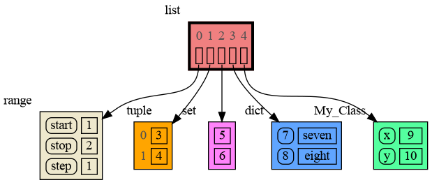
For program understanding and debugging, the [memory_graph](https://pypi.org/project/memory-graph/) package can visualize your data, supporting many different data types, including but not limited to:
|
|
35
|
+
|
|
36
|
+
```python
|
|
37
|
+
import memory_graph as mg
|
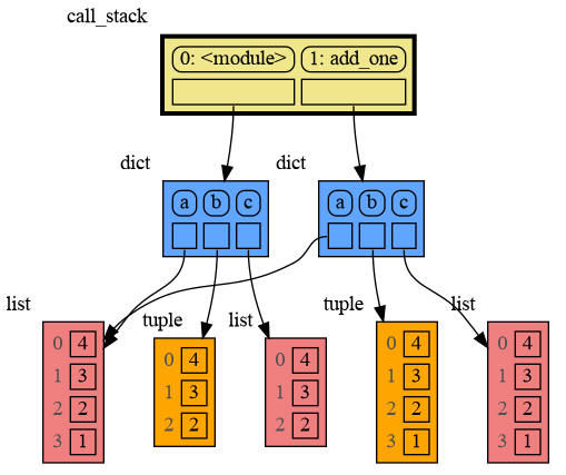
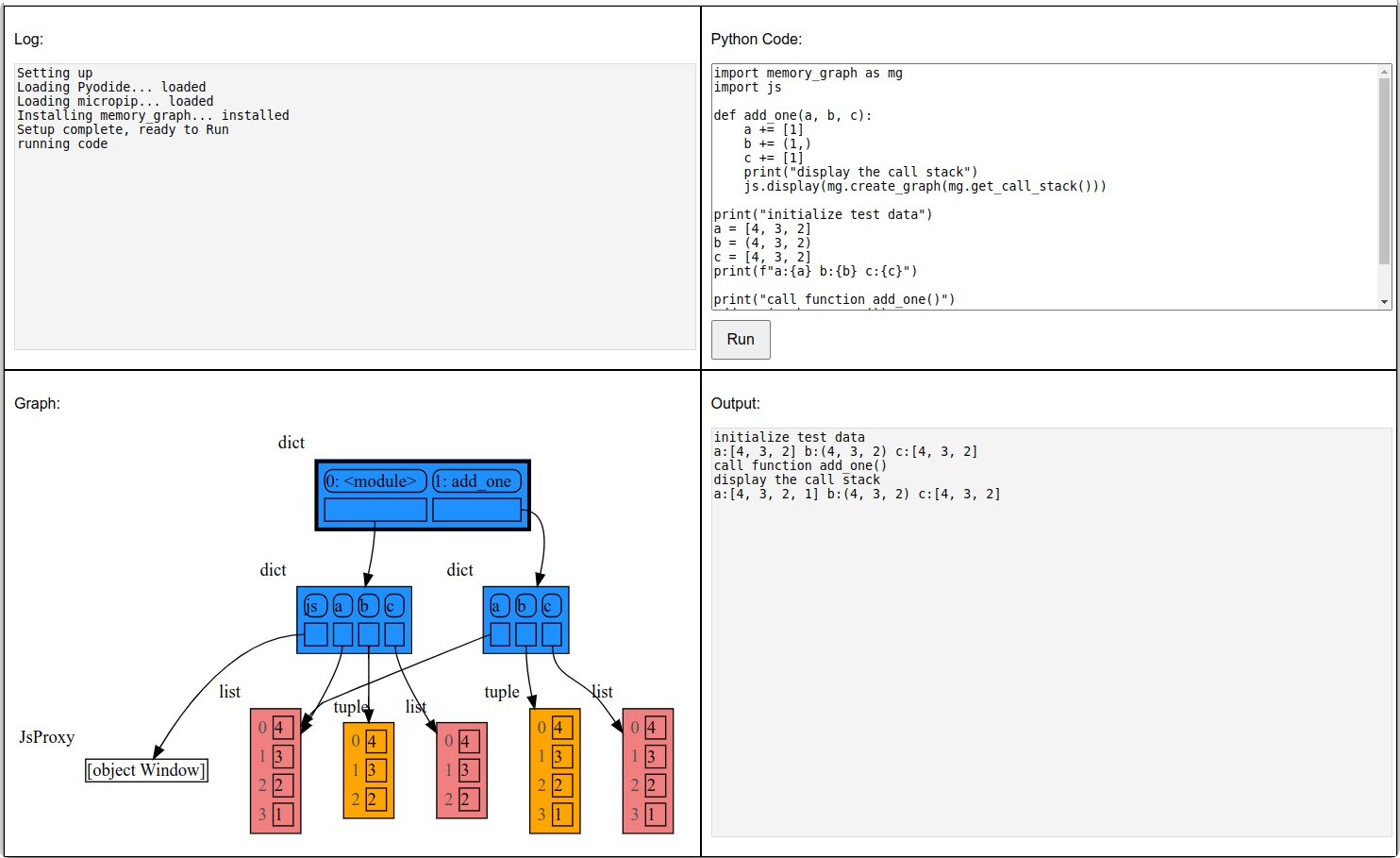
|
38
|
+
|
|
39
|
+
class My_Class:
|
|
40
|
+
|
|
41
|
+
def __init__(self, x, y):
|
|
42
|
+
self.x = x
|
|
43
|
+
self.y = y
|
|
44
|
+
|
|
45
|
+
data = [ range(1, 2), (3, 4), {5, 6}, {7:'seven', 8:'eight'}, My_Class(9, 10) ]
|
|
46
|
+
mg.show(data)
|
|
47
|
+
```
|
|
48
|
+
|
|
49
|
+
|
|
50
|
+
Instead of showing the graph on screen you can also render it to an output file (see [Graphviz Output Formats](https://graphviz.org/docs/outputs/)) using for example:
|
|
51
|
+
|
|
52
|
+
```python
|
|
53
|
+
mg.render(data, "my_graph.pdf")
|
|
54
|
+
mg.render(data, "my_graph.svg")
|
|
55
|
+
mg.render(data, "my_graph.png")
|
|
56
|
+
mg.render(data, "my_graph.gv") # Graphviz DOT file
|
|
57
|
+
mg.render(data) # renders to 'mg.render_filename' with default value: 'memory_graph.pdf'
|
|
58
|
+
```
|
|
59
|
+
|
|
60
|
+
# Sharing Values #
|
|
61
|
+
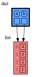
In Python, assigning the list from variable `a` to variable `b` causes both variables to reference the same list value and thus share it. Consequently, any change applied through one variable will impact the other. This behavior can lead to elusive bugs if a programmer incorrectly assumes that list `a` and `b` are independent.
|
|
62
|
+
|
|
63
|
+
<table><tr><td>
|
|
64
|
+
|
|
65
|
+
```python
|
|
66
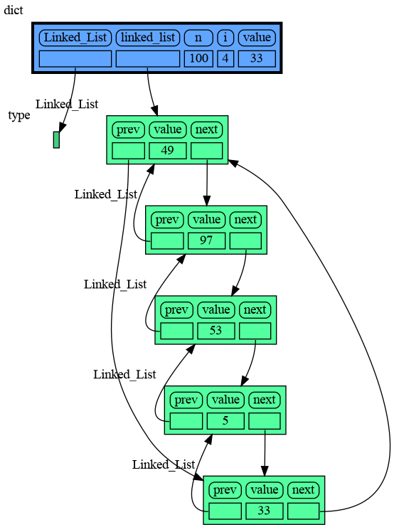
|
+
import memory_graph as mg
|
|
67
|
+
|
|
68
|
+
# create the lists 'a' and 'b'
|
|
69
|
+
a = [4, 3, 2]
|
|
70
|
+
b = a
|
|
71
|
+
b.append(1) # changing 'b' changes 'a'
|
|
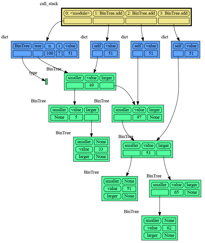
72
|
+
|
|
73
|
+
# print the 'a' and 'b' list
|
|
74
|
+
print('a:', a)
|
|
75
|
+
print('b:', b)
|
|
76
|
+
|
|
77
|
+
# check if 'a' and 'b' share data
|
|
78
|
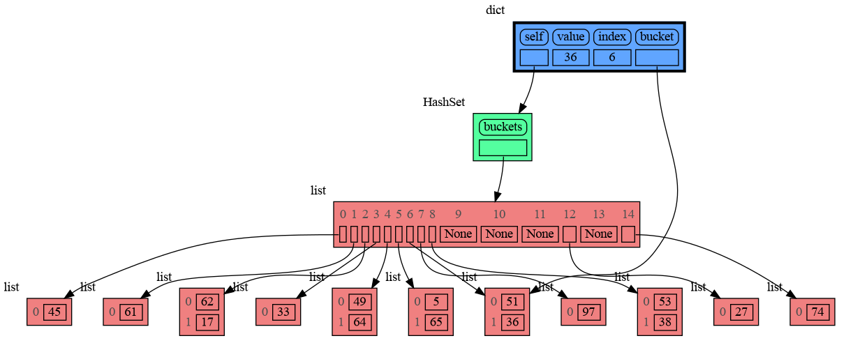
+
print('ids:', id(a), id(b))
|
|
79
|
+
print('identical?:', a is b)
|
|
80
|
+
|
|
81
|
+
# show all local variables in a graph
|
|
82
|
+
mg.show( locals() )
|
|
83
|
+
```
|
|
84
|
+
|
|
85
|
+
</td><td>
|
|
86
|
+
|
|
87
|
+
|
|
88
|
+
|
|
89
|
+
a graph showing `a` and `b` share data
|
|
90
|
+
|
|
91
|
+
</td></tr></table>
|
|
92
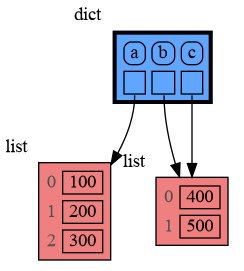
|
+
|
|
93
|
+
The fact that `a` and `b` share data can not be verified by printing the lists. It can be verified by comparing the identity of both variables using the `id()` function or by using the `is` comparison operator as shown in the program output below, but this quickly becomes impractical for larger programs.
|
|
94
|
+
```{verbatim}
|
|
95
|
+
a: 4, 3, 2, 1
|
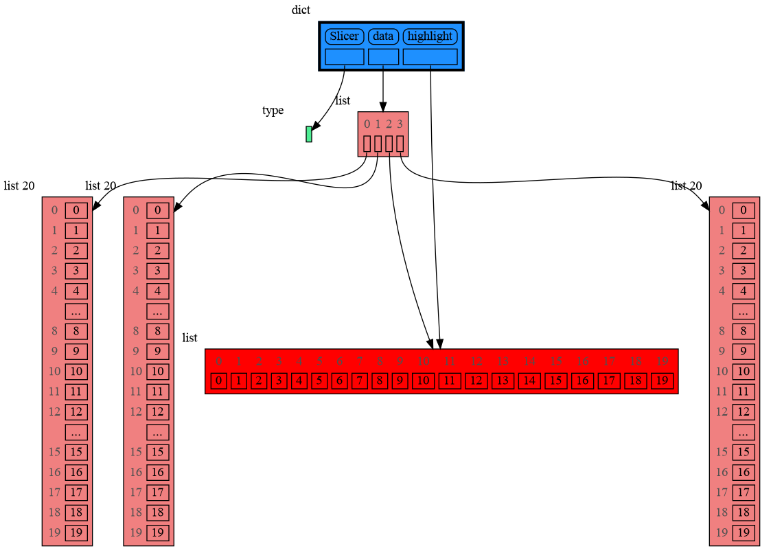
|
96
|
+
b: 4, 3, 2, 1
|
|
97
|
+
ids: 126432214913216 126432214913216
|
|
98
|
+
identical?: True
|
|
99
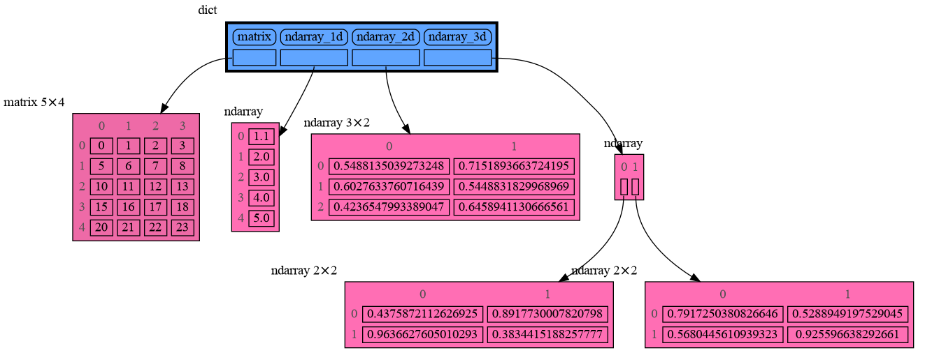
|
+
```
|
|
100
|
+
A better way to understand what data is shared is to draw a graph of the data using the [memory_graph](https://pypi.org/project/memory-graph/) package.
|
|
101
|
+
|
|
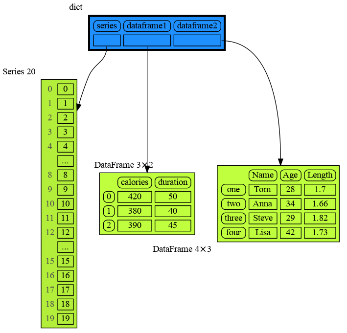
102
|
+
# Chapters #
|
|
103
|
+
|
|
104
|
+
[Python Data Model](#python-data-model)
|
|
105
|
+
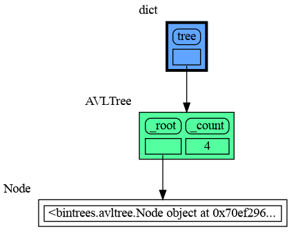
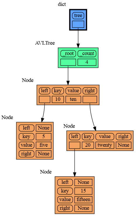
|
|
106
|
+
[Call Stack](#call-stack)
|
|
107
|
+
|
|
108
|
+
[Global Import Trick](#global-import-trick)
|
|
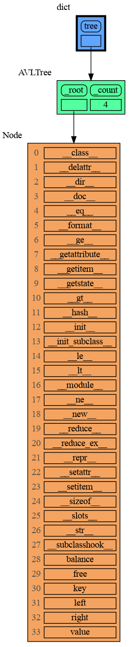
109
|
+
|
|
110
|
+
[Debugging](#debugging)
|
|
111
|
+
|
|
112
|
+
[Data Structure Examples](#data-structure-examples)
|
|
113
|
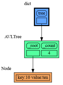
+
|
|
114
|
+
[Configuration](#configuration)
|
|
115
|
+
|
|
116
|
+
[Extensions](#extensions)
|
|
117
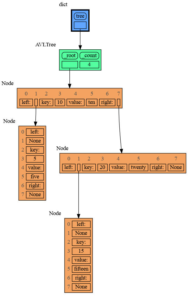
|
+
|
|
118
|
+
[Introspection](#introspection)
|
|
119
|
+
|
|
120
|
+
[Graph Depth](#graph-depth)
|
|
121
|
+
|
|
122
|
+
[Jupyter Notebook](#jupyter-notebook)
|
|
123
|
+
|
|
124
|
+
[ipython](#ipython)
|
|
125
|
+
|
|
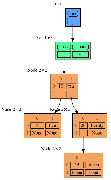
126
|
+
[In the Browser](#in-the-browser)
|
|
127
|
+
|
|
128
|
+
[Animated GIF](#animated-gif)
|
|
129
|
+
|
|
130
|
+
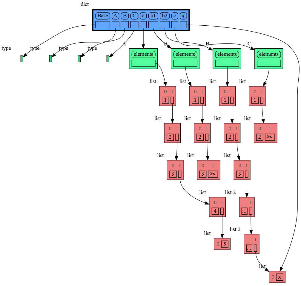
[Troubleshooting](#troubleshooting)
|
|
131
|
+
|
|
132
|
+
|
|
133
|
+
## Author ##
|
|
134
|
+
Bas Terwijn
|
|
135
|
+
|
|
136
|
+
## Inspiration ##
|
|
137
|
+
Inspired by [Python Tutor](https://pythontutor.com/).
|
|
138
|
+
|
|
139
|
+
## Supported by ##
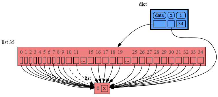
|
|
140
|
+
<img src="https://raw.githubusercontent.com/bterwijn/memory_graph/main/images/uva.png" alt="University of Amsterdam" width="600">
|
|
141
|
+
|
|
142
|
+
___
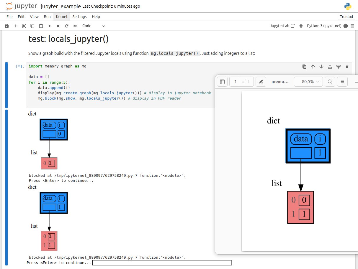
|
|
143
|
+
___
|
|
144
|
+
|
|
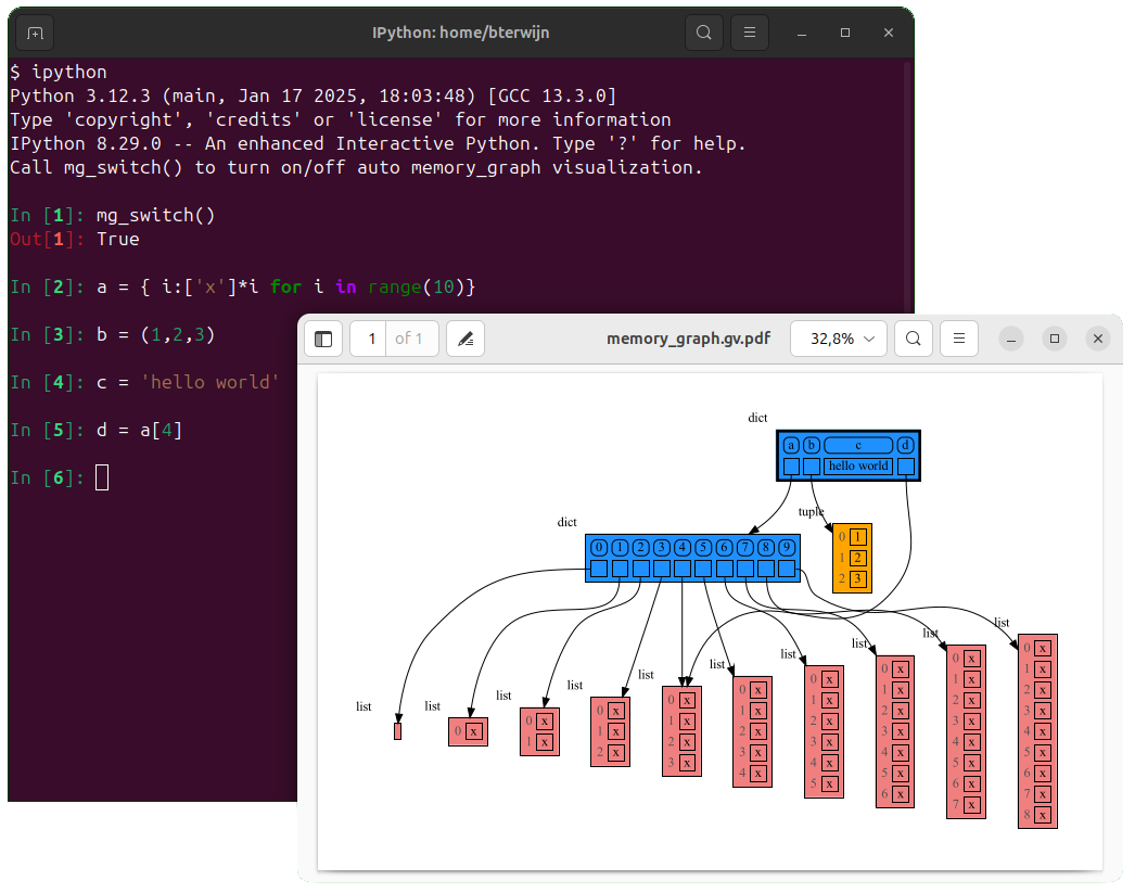
145
|
+
# Python Data Model #
|
|
146
|
+
The [Python Data Model](https://docs.python.org/3/reference/datamodel.html) makes a distiction between immutable and mutable types:
|
|
147
|
+
|
|
148
|
+
* **immutable**: bool, int, float, complex, str, tuple, bytes, frozenset
|
|
149
|
+
* **mutable**: list, set, dict, classes, ... (most other types)
|
|
150
|
+
|
|
151
|
+
|
|
152
|
+
## Immutable Type ##
|
|
153
|
+
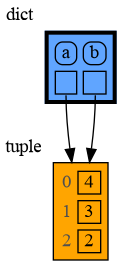
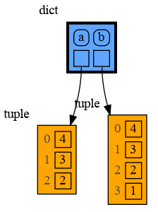
In the code below variable `a` and `b` both reference the same tuple value (4, 3, 2). A tuple is an immutable type and therefore when we change variable `b` its value **cannot** be mutated in place, and thus an automatic copy is made and `a` and `b` reference a different value afterwards.
|
|
154
|
+
|
|
155
|
+
```python
|
|
156
|
+
import memory_graph as mg
|
|
157
|
+
|
|
158
|
+
a = (4, 3, 2)
|
|
159
|
+
b = a
|
|
160
|
+
mg.render(locals(), 'immutable1.png')
|
|
161
|
+
|
|
162
|
+
b += (1,)
|
|
163
|
+
mg.render(locals(), 'immutable2.png')
|
|
164
|
+
```
|
|
165
|
+
|  |  |
|
|
166
|
+
|:-----------------------------------------------------------:|:-------------------------------------------------------------:|
|
|
167
|
+
| immutable1.png | immutable2.png |
|
|
168
|
+
|
|
169
|
+
|
|
170
|
+
## Mutable Type ##
|
|
171
|
+
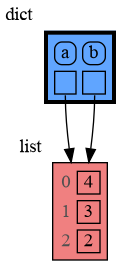
With mutable types the result is different. In the code below variable `a` and `b` both reference the same `list` value [4, 3, 2]. A `list` is a mutable type and therefore when we change variable `b` its value **can** be mutated in place and thus `a` and `b` both reference the same new value afterwards. Thus changing `b` also changes `a` and vice versa. Sometimes we want this but other times we don't and then we will have to make a copy ourselfs so that `a` and `b` are independent.
|
|
172
|
+
|
|
173
|
+
```python
|
|
174
|
+
import memory_graph as mg
|
|
175
|
+
|
|
176
|
+
a = [4, 3, 2]
|
|
177
|
+
b = a
|
|
178
|
+
mg.render(locals(), 'mutable1.png')
|
|
179
|
+
|
|
180
|
+
b += [1] # equivalent to: b.append(1)
|
|
181
|
+
mg.render(locals(), 'mutable2.png')
|
|
182
|
+
```
|
|
183
|
+
|  |  |
|
|
184
|
+
|:-----------------------------------------------------------:|:-------------------------------------------------------------:|
|
|
185
|
+
| mutable1.png | mutable2.png |
|
|
186
|
+
|
|
187
|
+
One practical reason why Python makes the distinction between mutable and immutable types is that a value of a mutable type can be large, making it inefficient to copy each time we change it. Immutable values generally don't need to change as much, or are small making copying less of a concern.
|
|
188
|
+
|
|
189
|
+
## Copying ##
|
|
190
|
+
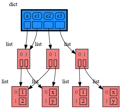
Python offers three different "copy" options that we will demonstrate using a nested list:
|
|
191
|
+
|
|
192
|
+
```python
|
|
193
|
+
import memory_graph as mg
|
|
194
|
+
import copy
|
|
195
|
+
|
|
196
|
+
a = [ [1, 2], ['x', 'y'] ] # a nested list (a list containing lists)
|
|
197
|
+
|
|
198
|
+
# three different ways to make a "copy" of 'a':
|
|
199
|
+
c1 = a
|
|
200
|
+
c2 = copy.copy(a) # equivalent to: a.copy() a[:] list(a)
|
|
201
|
+
c3 = copy.deepcopy(a)
|
|
202
|
+
|
|
203
|
+
mg.show(locals())
|
|
204
|
+
```
|
|
205
|
+
|
|
206
|
+
* `c1` is an **assignment**, nothing is copied, all the values are shared
|
|
207
|
+
* `c2` is a **shallow copy**, only the value referenced by the first reference is copied, all the underlying values are shared
|
|
208
|
+
* `c3` is a **deep copy**, all the values are copied, nothing is shared
|
|
209
|
+
|
|
210
|
+
|
|
211
|
+
|
|
212
|
+
|
|
213
|
+
## Custom Copy ##
|
|
214
|
+
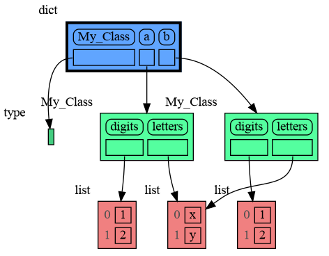
We can write our own custom copy function or method in case the three standard "copy" options don't do what we want. For example, in the code below the copy() method of My_Class copies the `digits` but shares the `letters` between two objects.
|
|
215
|
+
|
|
216
|
+
```python
|
|
217
|
+
import memory_graph as mg
|
|
218
|
+
import copy
|
|
219
|
+
|
|
220
|
+
class My_Class:
|
|
221
|
+
|
|
222
|
+
def __init__(self):
|
|
223
|
+
self.digits = [1, 2]
|
|
224
|
+
self.letters = ['x', 'y']
|
|
225
|
+
|
|
226
|
+
def custom_copy(self):
|
|
227
|
+
""" Copies 'digits' but shares 'letters'. """
|
|
228
|
+
c = copy.copy(self)
|
|
229
|
+
c.digits = copy.copy(self.digits)
|
|
230
|
+
return c
|
|
231
|
+
|
|
232
|
+
a = My_Class()
|
|
233
|
+
b = a.custom_copy()
|
|
234
|
+
|
|
235
|
+
mg.show(locals())
|
|
236
|
+
```
|
|
237
|
+
|
|
238
|
+
|
|
239
|
+
## Name Rebinding ##
|
|
240
|
+
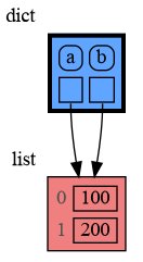
When `a` and `b` share a mutable value, then changing the value of `b` changes the value of `a` and vice versa. However, reassigning `b` does not change `a`. When you reassign `b`, you only rebind the name `b` to a new value without effecting any other variables.
|
|
241
|
+
|
|
242
|
+
```python
|
|
243
|
+
import memory_graph as mg
|
|
244
|
+
|
|
245
|
+
a = [4, 3, 2]
|
|
246
|
+
b = a
|
|
247
|
+
mg.render(locals(), 'rebinding1.png')
|
|
248
|
+
|
|
249
|
+
b += [1] # changes the value of 'b' and 'a'
|
|
250
|
+
b = [100, 200] # rebinds 'b' to a new value, 'a' is uneffected
|
|
251
|
+
mg.render(locals(), 'rebinding2.png')
|
|
252
|
+
```
|
|
253
|
+
|  |  |
|
|
254
|
+
|:-----------------------------------------------------------:|:-------------------------------------------------------------:|
|
|
255
|
+
| rebinding1.png | rebinding2.png |
|
|
256
|
+
|
|
257
|
+
# Call Stack #
|
|
258
|
+
The `mg.stack()` function retrieves the entire call stack, including the local variables for each function on the stack. This enables us to visualize the local variables across all active functions simultaneously. By examining the graph, we can determine whether any local variables from different functions share data. For instance, consider the function `add_one()` which adds the value `1` to each of its parameters `a`, `b`, and `c`.
|
|
259
|
+
|
|
260
|
+
```python
|
|
261
|
+
import memory_graph as mg
|
|
262
|
+
|
|
263
|
+
def add_one(a, b, c):
|
|
264
|
+
a += [1]
|
|
265
|
+
b += (1,)
|
|
266
|
+
c += [1]
|
|
267
|
+
mg.show(mg.stack())
|
|
268
|
+
|
|
269
|
+
a = [4, 3, 2]
|
|
270
|
+
b = (4, 3, 2)
|
|
271
|
+
c = [4, 3, 2]
|
|
272
|
+
|
|
273
|
+
add_one(a, b, c.copy())
|
|
274
|
+
print(f"a:{a} b:{b} c:{c}")
|
|
275
|
+
```
|
|
276
|
+
|
|
277
|
+
|
|
278
|
+
In the printed output only `a` is changed as a result of the function call:
|
|
279
|
+
```
|
|
280
|
+
a:[4, 3, 2, 1] b:(4, 3, 2) c:[4, 3, 2]
|
|
281
|
+
```
|
|
282
|
+
|
|
283
|
+
This is because `b` is of immutable type 'tuple' so its value gets copied automatically when it is changed. And because the function is called with a copy of `c`, its original value is not changed by the function. The value of variable `a` is the only value of mutable type that is shared between the root stack frame **'0: \<module>'** and the **'1: add_one'** stack frame of the function so only that variable is affected as a result of the function call. The other changes remain confined to the local variables of the ```add_one()``` function.
|
|
284
|
+
|
|
285
|
+
## Block ##
|
|
286
|
+
It is often helpful to temporarily block program execution to inspect the graph. For this we can use the `mg.block()` function:
|
|
287
|
+
|
|
288
|
+
```python
|
|
289
|
+
mg.block(fun, arg1, arg2, ...)
|
|
290
|
+
```
|
|
291
|
+
|
|
292
|
+
This function:
|
|
293
|
+
* first executes `fun(arg1, arg2, ...)`
|
|
294
|
+
* then prints the current source location in the program
|
|
295
|
+
* then blocks execution until the <Enter> key is pressed
|
|
296
|
+
* finally returns the value of the `fun()` call
|
|
297
|
+
|
|
298
|
+
To change its behavior:
|
|
299
|
+
* Set `mg.block_prints_location = False` to skip printing the source location.
|
|
300
|
+
* Set `mg.press_enter_message = None` to skip printing "Press <Enter> to continue...".
|
|
301
|
+
|
|
302
|
+
## Recursion ##
|
|
303
|
+
The call stack is also helpful to visualize how recursion works. Here we use `mg.block()` to show each step of how recursively ```factorial(3)``` is computed:
|
|
304
|
+
|
|
305
|
+
```python
|
|
306
|
+
import memory_graph as mg
|
|
307
|
+
|
|
308
|
+
def factorial(n):
|
|
309
|
+
if n==0:
|
|
310
|
+
return 1
|
|
311
|
+
mg.block(mg.show, mg.stack())
|
|
312
|
+
result = n * factorial(n-1)
|
|
313
|
+
mg.block(mg.show, mg.stack())
|
|
314
|
+
return result
|
|
315
|
+
|
|
316
|
+
print(factorial(3))
|
|
317
|
+
```
|
|
318
|
+
|
|
319
|
+
|
|
320
|
+
|
|
321
|
+
and the result is: 1 x 2 x 3 = 6
|
|
322
|
+
|
|
323
|
+
## Power Set ##
|
|
324
|
+
A more interesting recursive example that shows sharing of data is power_set(). A power set is the set of all subsets of a collection of values.
|
|
325
|
+
|
|
326
|
+
```python
|
|
327
|
+
import memory_graph as mg
|
|
328
|
+
|
|
329
|
+
def get_subsets(subsets, data, i, subset):
|
|
330
|
+
mg.block(mg.show, mg.stack())
|
|
331
|
+
if i == len(data):
|
|
332
|
+
subsets.append(subset.copy())
|
|
333
|
+
return
|
|
334
|
+
subset.append(data[i])
|
|
335
|
+
get_subsets(subsets, data, i+1, subset) # do include data[i]
|
|
336
|
+
subset.pop()
|
|
337
|
+
get_subsets(subsets, data, i+1, subset) # don't include data[i]
|
|
338
|
+
mg.block(mg.show, mg.stack())
|
|
339
|
+
|
|
340
|
+
def power_set(data):
|
|
341
|
+
subsets = []
|
|
342
|
+
get_subsets(subsets, data, 0, [])
|
|
343
|
+
return subsets
|
|
344
|
+
|
|
345
|
+
print( power_set(['a', 'b', 'c']) )
|
|
346
|
+
```
|
|
347
|
+
|
|
348
|
+
|
|
349
|
+
```
|
|
350
|
+
[['a', 'b', 'c'], ['a', 'b'], ['a', 'c'], ['a'], ['b', 'c'], ['b'], ['c'], []]
|
|
351
|
+
```
|
|
352
|
+
|
|
353
|
+
# Debugging #
|
|
354
|
+
|
|
355
|
+
For the best debugging experience with memory_graph set for example expression:
|
|
356
|
+
```
|
|
357
|
+
mg.render(locals(), "my_graph.pdf")
|
|
358
|
+
```
|
|
359
|
+
as a *watch* in a debugger tool such as the integrated debugger in Visual Studio Code. Then open the "my_graph.pdf" output file to continuously see all the local variables while debugging. This avoids having to add any memory_graph `show()` or `render()` calls to your code.
|
|
360
|
+
|
|
361
|
+
## Call Stack in Watch Context ##
|
|
362
|
+
The ```mg.stack()``` doesn't work well in *watch* context in most debuggers because debuggers introduce additional stack frames that cause problems. Use these alternative functions for various debuggers to filter out these problematic stack frames:
|
|
363
|
+
|
|
364
|
+
| debugger | function to get the call stack |
|
|
365
|
+
|:---|:---|
|
|
366
|
+
| **pdb, pudb** | `mg.stack_pdb()` |
|
|
367
|
+
| **Visual Studio Code** | `mg.stack_vscode()` |
|
|
368
|
+
| **Cursor AI** | `mg.stack_cursor()` |
|
|
369
|
+
| **PyCharm** | `mg.stack_pycharm()` |
|
|
370
|
+
|
|
371
|
+
|
|
372
|
+
|
|
373
|
+
## Other Debuggers ##
|
|
374
|
+
For other debuggers, invoke this function within the *watch* context. Then, in the "call_stack.txt" file, identify the slice of functions you wish to include as stack frames in the call stack.
|
|
375
|
+
```
|
|
376
|
+
mg.save_call_stack("call_stack.txt")
|
|
377
|
+
```
|
|
378
|
+
Choose 'after' and 'through' what function you want to slice and then call this function to get the desired call stack. The `drop` argument can optionally be used to drop a number of stack frames after the `after_function`:
|
|
379
|
+
```
|
|
380
|
+
mg.stack_after_through(after_function, through_function="<module>", drop=0)
|
|
381
|
+
```
|
|
382
|
+
|
|
383
|
+
## Debugging without Debugger Tool ##
|
|
384
|
+
|
|
385
|
+
To simplify debugging without a debugger tool, we offer these alias functions that you can insert into your code at the point where you want to visualize a graph:
|
|
386
|
+
|
|
387
|
+
| alias | purpose | function call |
|
|
388
|
+
|:---|:---|:---|
|
|
389
|
+
| `mg.sl()` | **s**how **l**ocal variables | `mg.show(locals())` |
|
|
390
|
+
| `mg.ss()` | **s**how the call **s**tack | `mg.show(mg.stack())` |
|
|
391
|
+
| `mg.bsl()` | **b**lock after **s**howing **l**ocal variables | `mg.block(mg.show, locals())` |
|
|
392
|
+
| `mg.bss()` | **b**lock after **s**howing the call **s**tack | `mg.block(mg.show, mg.stack())` |
|
|
393
|
+
| `mg.rl()` | **r**ender **l**ocal variables | `mg.render(locals())` |
|
|
394
|
+
| `mg.rs()` | **r**ender the call **s**tack | `mg.render(mg.stack())` |
|
|
395
|
+
| `mg.brl()` | **b**lock after **r**endering **l**ocal variables | `mg.block(mg.render, locals())` |
|
|
396
|
+
| `mg.brs()` | **b**lock after **r**endering the call **s**tack | `mg.block(mg.render, mg.stack())` |
|
|
397
|
+
| `mg.l()` | same as `mg.bsl()` | |
|
|
398
|
+
| `mg.s()` | same as `mg.bss()` | |
|
|
399
|
+
|
|
400
|
+
For example, executing this program:
|
|
401
|
+
|
|
402
|
+
```python
|
|
403
|
+
from memory_graph as mg
|
|
404
|
+
|
|
405
|
+
squares = []
|
|
406
|
+
squares_collector = []
|
|
407
|
+
for i in range(1, 6):
|
|
408
|
+
squares.append(i**2)
|
|
409
|
+
squares_collector.append(squares.copy())
|
|
410
|
+
mg.l() # block after showing local variables
|
|
411
|
+
```
|
|
412
|
+
and pressing <Enter> a number of times, results in:
|
|
413
|
+
|
|
414
|
+
|
|
415
|
+
|
|
416
|
+
# Data Structure Examples #
|
|
417
|
+
Module memory_graph can be very useful in a course about data structures, some examples:
|
|
418
|
+
|
|
419
|
+
## Circular Doubly Linked List ##
|
|
420
|
+
```python
|
|
421
|
+
import memory_graph as mg
|
|
422
|
+
import random
|
|
423
|
+
random.seed(0) # use same random numbers each run
|
|
424
|
+
|
|
425
|
+
class Linked_List:
|
|
426
|
+
""" Circular doubly linked list """
|
|
427
|
+
|
|
428
|
+
def __init__(self, value=None,
|
|
429
|
+
prev=None, next=None):
|
|
430
|
+
self.prev = prev if prev else self
|
|
431
|
+
self.value = value
|
|
432
|
+
self.next = next if next else self
|
|
433
|
+
|
|
434
|
+
def add_back(self, value):
|
|
435
|
+
if self.value == None:
|
|
436
|
+
self.value = value
|
|
437
|
+
else:
|
|
438
|
+
new_node = Linked_List(value,
|
|
439
|
+
prev=self.prev,
|
|
440
|
+
next=self)
|
|
441
|
+
self.prev.next = new_node
|
|
442
|
+
self.prev = new_node
|
|
443
|
+
|
|
444
|
+
linked_list = Linked_List()
|
|
445
|
+
n = 100
|
|
446
|
+
for i in range(n):
|
|
447
|
+
value = random.randrange(n)
|
|
448
|
+
linked_list.add_back(value)
|
|
449
|
+
mg.block(mg.show, locals()) # <--- draw locals
|
|
450
|
+
```
|
|
451
|
+
|
|
452
|
+
|
|
453
|
+
## Binary Tree ##
|
|
454
|
+
```python
|
|
455
|
+
import memory_graph as mg
|
|
456
|
+
import random
|
|
457
|
+
random.seed(0) # use same random numbers each run
|
|
458
|
+
|
|
459
|
+
class BinTree:
|
|
460
|
+
|
|
461
|
+
def __init__(self, value=None, smaller=None, larger=None):
|
|
462
|
+
self.smaller = smaller
|
|
463
|
+
self.value = value
|
|
464
|
+
self.larger = larger
|
|
465
|
+
|
|
466
|
+
def add(self, value):
|
|
467
|
+
if self.value is None:
|
|
468
|
+
self.value = value
|
|
469
|
+
elif value < self.value:
|
|
470
|
+
if self.smaller is None:
|
|
471
|
+
self.smaller = BinTree(value)
|
|
472
|
+
else:
|
|
473
|
+
self.smaller.add(value)
|
|
474
|
+
else:
|
|
475
|
+
if self.larger is None:
|
|
476
|
+
self.larger = BinTree(value)
|
|
477
|
+
else:
|
|
478
|
+
self.larger.add(value)
|
|
479
|
+
mg.block(mg.show, mg.stack()) # <--- draw stack
|
|
480
|
+
|
|
481
|
+
tree = BinTree()
|
|
482
|
+
n = 100
|
|
483
|
+
for i in range(n):
|
|
484
|
+
value = random.randrange(n)
|
|
485
|
+
tree.add(value)
|
|
486
|
+
```
|
|
487
|
+
|
|
488
|
+
|
|
489
|
+
## Hash Set ##
|
|
490
|
+
```python
|
|
491
|
+
import memory_graph as mg
|
|
492
|
+
import random
|
|
493
|
+
random.seed(0) # use same random numbers each run
|
|
494
|
+
|
|
495
|
+
class HashSet:
|
|
496
|
+
|
|
497
|
+
def __init__(self, capacity=15):
|
|
498
|
+
self.buckets = [None] * capacity
|
|
499
|
+
|
|
500
|
+
def add(self, value):
|
|
501
|
+
index = hash(value) % len(self.buckets)
|
|
502
|
+
if self.buckets[index] is None:
|
|
503
|
+
self.buckets[index] = []
|
|
504
|
+
bucket = self.buckets[index]
|
|
505
|
+
bucket.append(value)
|
|
506
|
+
mg.block(mg.show, locals()) # <--- draw locals
|
|
507
|
+
|
|
508
|
+
def contains(self, value):
|
|
509
|
+
index = hash(value) % len(self.buckets)
|
|
510
|
+
if self.buckets[index] is None:
|
|
511
|
+
return False
|
|
512
|
+
return value in self.buckets[index]
|
|
513
|
+
|
|
514
|
+
def remove(self, value):
|
|
515
|
+
index = hash(value) % len(self.buckets)
|
|
516
|
+
if self.buckets[index] is not None:
|
|
517
|
+
self.buckets[index].remove(value)
|
|
518
|
+
|
|
519
|
+
hash_set = HashSet()
|
|
520
|
+
n = 100
|
|
521
|
+
for i in range(n):
|
|
522
|
+
new_value = random.randrange(n)
|
|
523
|
+
hash_set.add(new_value)
|
|
524
|
+
```
|
|
525
|
+
|
|
526
|
+
|
|
527
|
+
|
|
528
|
+
# Configuration #
|
|
529
|
+
Different aspects of memory_graph can be configured. The default configuration is reset by importing 'memory_graph.config_default'.
|
|
530
|
+
|
|
531
|
+
- ***mg.config.max_string_length*** : int
|
|
532
|
+
- The maximum length of strings shown in the graph. Longer strings will be truncated.
|
|
533
|
+
|
|
534
|
+
- ***mg.config.not_node_types*** : set[type]
|
|
535
|
+
- Holds all types for which no seperate node is drawn but that instead are shown as elements in their parent Node.
|
|
536
|
+
|
|
537
|
+
- ***mg.config.no_child_references_types*** : set[type]
|
|
538
|
+
- The set of key_value types that don't draw references to their direct childeren but have their children shown as elements of their node.
|
|
539
|
+
|
|
540
|
+
- ***mg.config.type_to_node*** : dict[type, fun(data) -> Node]
|
|
541
|
+
- Determines how a data types is converted to a Node (sub)class for visualization in the graph.
|
|
542
|
+
|
|
543
|
+
- ***mg.config.type_to_color*** : dict[type, color]
|
|
544
|
+
- Maps a type to the [graphviz color](https://graphviz.org/doc/info/colors.html) it gets in the graph.
|
|
545
|
+
|
|
546
|
+
- ***mg.config.type_to_vertical_orientation*** : dict[type, bool]
|
|
547
|
+
- Maps a type to its orientation. Use 'True' for vertical and 'False' for horizontal. If not specified Node_Linear and Node_Key_Value are vertical unless they have references to children.
|
|
548
|
+
|
|
549
|
+
- ***mg.config.type_to_slicer*** : dict[type, int]
|
|
550
|
+
- Maps a type to a Slicer. A slicer determines how many elements of a data type are shown in the graph to prevent the graph from getting too big. 'Slicer()' does no slicing, 'Slicer(1,2,3)' shows just 1 element at the beginning, 2 in the middle, and 3 at the end.
|
|
551
|
+
|
|
552
|
+
- ***mg.config.max_graph_depth*** : int
|
|
553
|
+
- The maxium depth of the graph with default value 12.
|
|
554
|
+
|
|
555
|
+
- ***config.graph_cut_symbol*** : str
|
|
556
|
+
- The symbol indicating where the graph is cut short with default `✂`.
|
|
557
|
+
|
|
558
|
+
- ***mg.config.type_to_depth*** : dict[type, int]
|
|
559
|
+
- Maps a type to graph depth to limit the graph size.
|
|
560
|
+
|
|
561
|
+
- ***max_missing_edges*** : int
|
|
562
|
+
- Maximum number of missing edges that are shown with default value 2. Dashed references are used to indicate that there are more references to a node than are shown.
|
|
563
|
+
|
|
564
|
+
|
|
565
|
+
## Simplified Graph ##
|
|
566
|
+
Memory_graph simplifies the visualization (and the viewer's mental model) by **not** showing separate nodes for immutable types like `bool`, `int`, `float`, `complex`, and `str` by default. This simplification can sometimes be slightly misleading. As in the example below, after a shallow copy, lists `a` and `b` technically share their `int` values, but the graph makes it appear as though `a` and `b` each have their own copies. However, since `int` is immutable, this simplification will never lead to unexpected changes (changing `a` won’t affect `b`) so will never result in bugs.
|
|
567
|
+
|
|
568
|
+
The simplification strikes a balance: it is slightly misleading but keeps the graph clean and easy to understand and focuses on the mutable types where unexpected changes can occur. This is why it is the default behavior. If you do want to show separate nodes for `int` values, such as for educational purposes, you can simply remove `int` from the `mg.config.not_node_types` set:
|
|
569
|
+
```python
|
|
570
|
+
import memory_graph as mg
|
|
571
|
+
|
|
572
|
+
a = [100, 200, 300]
|
|
573
|
+
b = a.copy()
|
|
574
|
+
mg.render(locals(), 'not_node_types1.png')
|
|
575
|
+
|
|
576
|
+
mg.config.not_node_types.remove(int) # now show separate nodes for int values
|
|
577
|
+
|
|
578
|
+
mg.render(locals(), 'not_node_types2.png')
|
|
579
|
+
```
|
|
580
|
+
|  |  |
|
|
581
|
+
|:-----------------------------------------------------------:|:-------------------------------------------------------------:|
|
|
582
|
+
| not_node_types1.png — simplified | not_node_types2.png — technically correct |
|
|
583
|
+
|
|
584
|
+
Additionally, the simplification hides away the [reuse of small int values \[-5, 256\]](https://docs.python.org/3/c-api/long.html#c.PyLong_FromLong) in the current CPython implementation, an optimization that might otherwise confuse beginner Python programmers. For instance, after executing `a[1]+=1; b[1]+=1` the `201` value is, maybe surprisingly, still shared between `a` and `b`, whereas executing `a[2]+=1; b[2]+=1` does not result in sharing the `301` value.
|
|
585
|
+
|
|
586
|
+
## Temporary Configuration ##
|
|
587
|
+
In addition to the global configuration, a temporary configuration can be set for a single `show()` or `render()` call to change the colors, orientation, and slicer. This example highlights a particular list element in red, gives it a horizontal orientation, and overwrites the default slicer for lists:
|
|
588
|
+
|
|
589
|
+
```python
|
|
590
|
+
import memory_graph as mg
|
|
591
|
+
from memory_graph.slicer import Slicer
|
|
592
|
+
|
|
593
|
+
data = [ list(range(20)) for i in range(1,5)]
|
|
594
|
+
highlight = data[2]
|
|
595
|
+
|
|
596
|
+
mg.show( locals(),
|
|
597
|
+
colors = {id(highlight): "red" }, # set color to red
|
|
598
|
+
vertical_orientations = {id(highlight): False }, # set horizontal orientation
|
|
599
|
+
slicers = {id(highlight): Slicer()} # set no slicing
|
|
600
|
+
)
|
|
601
|
+
```
|
|
602
|
+
|
|
603
|
+
|
|
604
|
+
# Extensions #
|
|
605
|
+
Different extensions are available for types from other Python packages.
|
|
606
|
+
|
|
607
|
+
## Numpy ##
|
|
608
|
+
Numpy types `array` and `matrix` and `ndarray` can be graphed with "memory_graph.extension_numpy":
|
|
609
|
+
|
|
610
|
+
```python
|
|
611
|
+
import memory_graph as mg
|
|
612
|
+
import numpy as np
|
|
613
|
+
import memory_graph.extension_numpy
|
|
614
|
+
np.random.seed(0) # use same random numbers each run
|
|
615
|
+
|
|
616
|
+
array = np.array([1.1, 2, 3, 4, 5])
|
|
617
|
+
matrix = np.matrix([[i*20+j for j in range(20)] for i in range(20)])
|
|
618
|
+
ndarray = np.random.rand(20,20)
|
|
619
|
+
mg.show(locals())
|
|
620
|
+
```
|
|
621
|
+
|
|
622
|
+
|
|
623
|
+
## Pandas ##
|
|
624
|
+
Pandas types `Series` and `DataFrame` can be graphed with "memory_graph.extension_pandas":
|
|
625
|
+
|
|
626
|
+
```python
|
|
627
|
+
import memory_graph as mg
|
|
628
|
+
import pandas as pd
|
|
629
|
+
import memory_graph.extension_pandas
|
|
630
|
+
|
|
631
|
+
series = pd.Series( [i for i in range(20)] )
|
|
632
|
+
dataframe1 = pd.DataFrame({ "calories": [420, 380, 390],
|
|
633
|
+
"duration": [50, 40, 45] })
|
|
634
|
+
dataframe2 = pd.DataFrame({ 'Name' : [ 'Tom', 'Anna', 'Steve', 'Lisa'],
|
|
635
|
+
'Age' : [ 28, 34, 29, 42],
|
|
636
|
+
'Length' : [ 1.70, 1.66, 1.82, 1.73] },
|
|
637
|
+
index=['one', 'two', 'three', 'four']) # with row names
|
|
638
|
+
mg.show(locals())
|
|
639
|
+
```
|
|
640
|
+
|
|
641
|
+
|
|
642
|
+
# Introspection #
|
|
643
|
+
This section is likely to change. Sometimes the introspection fails or is not as desired. For example the `bintrees.avltree.Node` object doesn't show any attributes in the graph below.
|
|
644
|
+
|
|
645
|
+
```python
|
|
646
|
+
import memory_graph as mg
|
|
647
|
+
import bintrees
|
|
648
|
+
|
|
649
|
+
# Create an AVL tree
|
|
650
|
+
tree = bintrees.AVLTree()
|
|
651
|
+
tree.insert(10, "ten")
|
|
652
|
+
tree.insert(5, "five")
|
|
653
|
+
tree.insert(20, "twenty")
|
|
654
|
+
tree.insert(15, "fifteen")
|
|
655
|
+
|
|
656
|
+
mg.show(locals())
|
|
657
|
+
```
|
|
658
|
+
|
|
659
|
+
|
|
660
|
+
|
|
661
|
+
## All attributes using dir() ##
|
|
662
|
+
A useful start is to give it some color, show the list of all its attributes using `dir()`, and setting an empty Slicer to see the attribute list in full.
|
|
663
|
+
|
|
664
|
+
```python
|
|
665
|
+
import memory_graph as mg
|
|
666
|
+
import bintrees
|
|
667
|
+
|
|
668
|
+
# Create an AVL tree
|
|
669
|
+
tree = bintrees.AVLTree()
|
|
670
|
+
tree.insert(10, "ten")
|
|
671
|
+
tree.insert(5, "five")
|
|
672
|
+
tree.insert(20, "twenty")
|
|
673
|
+
tree.insert(15, "fifteen")
|
|
674
|
+
|
|
675
|
+
mg.config.type_to_color[bintrees.avltree.Node] = "sandybrown"
|
|
676
|
+
mg.config.type_to_node[bintrees.avltree.Node] = lambda data: mg.node_linear.Node_Linear(data,
|
|
677
|
+
dir(data))
|
|
678
|
+
mg.config.type_to_slicer[bintrees.avltree.Node] = mg.slicer.Slicer()
|
|
679
|
+
|
|
680
|
+
mg.show(locals())
|
|
681
|
+
```
|
|
682
|
+
|
|
683
|
+
|
|
684
|
+
Next figure out what are the attributes you want to graph and choose a Node type, there are four options:
|
|
685
|
+
|
|
686
|
+
## 1) Node_Leaf ##
|
|
687
|
+
Node_Leaf is a node with no children and shows just a single value.
|
|
688
|
+
```python
|
|
689
|
+
import memory_graph as mg
|
|
690
|
+
import bintrees
|
|
691
|
+
|
|
692
|
+
# Create an AVL tree
|
|
693
|
+
tree = bintrees.AVLTree()
|
|
694
|
+
tree.insert(10, "ten")
|
|
695
|
+
tree.insert(5, "five")
|
|
696
|
+
tree.insert(20, "twenty")
|
|
697
|
+
tree.insert(15, "fifteen")
|
|
698
|
+
|
|
699
|
+
mg.config.type_to_color[bintrees.avltree.Node] = "sandybrown"
|
|
700
|
+
mg.config.type_to_node[bintrees.avltree.Node] = lambda data: mg.node_leaf.Node_Leaf(data,
|
|
701
|
+
f"key:{data.key} value:{data.value}")
|
|
702
|
+
|
|
703
|
+
mg.show(locals())
|
|
704
|
+
```
|
|
705
|
+
|
|
706
|
+
|
|
707
|
+
## 2) Node_Linear ##
|
|
708
|
+
Node_Linear shows multiple values in a line like a list.
|
|
709
|
+
```python
|
|
710
|
+
import memory_graph as mg
|
|
711
|
+
import bintrees
|
|
712
|
+
|
|
713
|
+
# Create an AVL tree
|
|
714
|
+
tree = bintrees.AVLTree()
|
|
715
|
+
tree.insert(10, "ten")
|
|
716
|
+
tree.insert(5, "five")
|
|
717
|
+
tree.insert(20, "twenty")
|
|
718
|
+
tree.insert(15, "fifteen")
|
|
719
|
+
|
|
720
|
+
mg.config.type_to_color[bintrees.avltree.Node] = "sandybrown"
|
|
721
|
+
mg.config.type_to_node[bintrees.avltree.Node] = lambda data: mg.node_linear.Node_Linear(data,
|
|
722
|
+
['left:', data.left,
|
|
723
|
+
'key:', data.key,
|
|
724
|
+
'value:', data.value,
|
|
725
|
+
'right:', data.right] )
|
|
726
|
+
|
|
727
|
+
mg.show(locals())
|
|
728
|
+
```
|
|
729
|
+
|
|
730
|
+
|
|
731
|
+
## 3) Node_Key_Value ##
|
|
732
|
+
Node_Key_Value shows key-value pairs like a dictionary. Note the required `items()` call at the end.
|
|
733
|
+
```python
|
|
734
|
+
import memory_graph as mg
|
|
735
|
+
import bintrees
|
|
736
|
+
|
|
737
|
+
# Create an AVL tree
|
|
738
|
+
tree = bintrees.AVLTree()
|
|
739
|
+
tree.insert(10, "ten")
|
|
740
|
+
tree.insert(5, "five")
|
|
741
|
+
tree.insert(20, "twenty")
|
|
742
|
+
tree.insert(15, "fifteen")
|
|
743
|
+
|
|
744
|
+
mg.config.type_to_color[bintrees.avltree.Node] = "sandybrown"
|
|
745
|
+
mg.config.type_to_node[bintrees.avltree.Node] = lambda data: mg.node_key_value.Node_Key_Value(data,
|
|
746
|
+
{'left': data.left,
|
|
747
|
+
'key': data.key,
|
|
748
|
+
'value': data.value,
|
|
749
|
+
'right': data.right}.items() )
|
|
750
|
+
|
|
751
|
+
mg.show(locals())
|
|
752
|
+
```
|
|
753
|
+
|
|
754
|
+
|
|
755
|
+
## 4) Node_Table ##
|
|
756
|
+
Node_Table shows all the values as a table.
|
|
757
|
+
```python
|
|
758
|
+
import memory_graph as mg
|
|
759
|
+
import bintrees
|
|
760
|
+
|
|
761
|
+
# Create an AVL tree
|
|
762
|
+
tree = bintrees.AVLTree()
|
|
763
|
+
tree.insert(10, "ten")
|
|
764
|
+
tree.insert(5, "five")
|
|
765
|
+
tree.insert(20, "twenty")
|
|
766
|
+
tree.insert(15, "fifteen")
|
|
767
|
+
|
|
768
|
+
mg.config.type_to_color[bintrees.avltree.Node] = "sandybrown"
|
|
769
|
+
mg.config.type_to_node[bintrees.avltree.Node] = lambda data: mg.node_table.Node_Table(data,
|
|
770
|
+
[[data.key, data.value],
|
|
771
|
+
[data.left, data.right]] )
|
|
772
|
+
|
|
773
|
+
|
|
774
|
+
mg.show(locals())
|
|
775
|
+
```
|
|
776
|
+
|
|
777
|
+
|
|
778
|
+
|
|
779
|
+
# Graph Depth #
|
|
780
|
+
To limit the size of the graph the maximum depth of the graph is set by `mg.config.max_graph_depth`. Additionally for each type a depth can be set to further limit the graph, as is done for type `B` in the example below. Scissors indicate where the graph is cut short. Alternatively the `id()` of a data elements can be used to limit the graph for that specific element, as is done for the value referenced by variable `c`.
|
|
781
|
+
|
|
782
|
+
The value of variable `x` is shown as it is at depth 1 from the root of the graph, but as it can also be reached via `b2`, that path need to be shown as well to avoid confusion, so this overwrites the depth limit set for type `B`.
|
|
783
|
+
|
|
784
|
+
```python
|
|
785
|
+
import memory_graph as mg
|
|
786
|
+
|
|
787
|
+
class Base:
|
|
788
|
+
|
|
789
|
+
def __init__(self, n):
|
|
790
|
+
self.elements = [1]
|
|
791
|
+
iter = self.elements
|
|
792
|
+
for i in range(2,n):
|
|
793
|
+
iter.append([i])
|
|
794
|
+
iter = iter[-1]
|
|
795
|
+
|
|
796
|
+
def get_last(self):
|
|
797
|
+
iter = self.elements
|
|
798
|
+
while len(iter)>1:
|
|
799
|
+
iter = iter[-1]
|
|
800
|
+
return iter
|
|
801
|
+
|
|
802
|
+
class A(Base):
|
|
803
|
+
|
|
804
|
+
def __init__(self, n):
|
|
805
|
+
super().__init__(n)
|
|
806
|
+
|
|
807
|
+
class B(Base):
|
|
808
|
+
|
|
809
|
+
def __init__(self, n):
|
|
810
|
+
super().__init__(n)
|
|
811
|
+
|
|
812
|
+
class C(Base):
|
|
813
|
+
|
|
814
|
+
def __init__(self, n):
|
|
815
|
+
super().__init__(n)
|
|
816
|
+
|
|
817
|
+
a = A(6)
|
|
818
|
+
b1 = B(6)
|
|
819
|
+
b2 = B(6)
|
|
820
|
+
c = C(6)
|
|
821
|
+
|
|
822
|
+
x = ['x']
|
|
823
|
+
b2.get_last().append(x)
|
|
824
|
+
|
|
825
|
+
mg.config.type_to_depth[B] = 3
|
|
826
|
+
mg.config.type_to_depth[id(c)] = 2
|
|
827
|
+
mg.show(locals())
|
|
828
|
+
```
|
|
829
|
+
|
|
830
|
+
|
|
831
|
+
## Hidden Edges ##
|
|
832
|
+
|
|
833
|
+
As the value of `x` is shown in the graph, we would want to show all the references to it, but the default list Slicer hides references by slicing the list to keep the graph small. The `max_missing_edges` variable then determines how many additional hidden references to `x` we show. If there are more references then we show, then theses hidden references are shown with dashed lines to indicate some references are left out.
|
|
834
|
+
|
|
835
|
+
```python
|
|
836
|
+
import memory_graph as mg
|
|
837
|
+
|
|
838
|
+
data = []
|
|
839
|
+
x = ['x']
|
|
840
|
+
for i in range(20):
|
|
841
|
+
data.append(x)
|
|
842
|
+
|
|
843
|
+
mg.show(locals())
|
|
844
|
+
```
|
|
845
|
+
|
|
846
|
+
|
|
847
|
+
# Jupyter Notebook #
|
|
848
|
+
In Jupyter Notebook `locals()` has additional variables that cause problems in the graph, use `mg.locals_jupyter()` to get the local variables with these problematic variables filtered out. Use `mg.stack_jupyter()` to get the whole call stack with these variables filtered out.
|
|
849
|
+
|
|
850
|
+
We can use `mg.show()` and `mg.render()` in a Jupyter Notebook, but alternatively we can also use `mg.create_graph()` to create a graph and the `display()` function to render it inline with for example:
|
|
851
|
+
|
|
852
|
+
```python
|
|
853
|
+
display( mg.create_graph(mg.locals_jupyter()) ) # display the local variables inline
|
|
854
|
+
mg.block(display, mg.create_graph(mg.locals_jupyter()) ) # the same but blocked
|
|
855
|
+
```
|
|
856
|
+
|
|
857
|
+
See for example [jupyter_example.ipynb](https://raw.githubusercontent.com/bterwijn/memory_graph/main/src/jupyter_example.ipynb).
|
|
858
|
+
|
|
859
|
+
|
|
860
|
+
# ipython #
|
|
861
|
+
In ipython `locals()` has additional variables that cause problems in the graph, use `mg.locals_ipython()` to get the local variables with these problematic variables filtered out. Use `mg.stack_ipython()` to get the whole call stack with these variables filtered out.
|
|
862
|
+
|
|
863
|
+
Additionally install file [auto_memory_graph.py](https://raw.githubusercontent.com/bterwijn/memory_graph/main/src/auto_memory_graph.py) in the ipython startup directory:
|
|
864
|
+
* Linux/Mac: `~/.ipython/profile_default/startup/`
|
|
865
|
+
* Windows: `%USERPROFILE%\.ipython\profile_default\startup\`
|
|
866
|
+
|
|
867
|
+
Then after starting 'ipython' call function `mg_switch()` to turn on/off the automatic visualization of local variables after each command.
|
|
868
|
+
|
|
869
|
+
|
|
870
|
+
# In the Browser #
|
|
871
|
+
We can also run memory_graph in the browser: <a href="https://bterwijn.github.io/memory_graph/src/pyodide.html" target="_blank">Pyodide Example</a>
|
|
872
|
+
|
|
873
|
+
|
|
874
|
+
|
|
875
|
+
# Animated GIF #
|
|
876
|
+
To make an animated GIF use for example `mg.show` or `mg.render` like this:
|
|
877
|
+
|
|
878
|
+
* mg.show(locals(), 'animated.png', numbered=True)
|
|
879
|
+
* mg.render(locals(), 'animated.png', numbered=True)
|
|
880
|
+
|
|
881
|
+
in your source or better as a *watch* in a debugger so that stepping through the code generates images:
|
|
882
|
+
|
|
883
|
+
animated0.png, animated1.png, animated2.png, ...
|
|
884
|
+
|
|
885
|
+
Then use these images to make an animated GIF, for example using this Bash script [create_gif.sh](https://raw.githubusercontent.com/bterwijn/memory_graph/main/images/create_gif.sh):
|
|
886
|
+
|
|
887
|
+
```bash
|
|
888
|
+
$ bash create_gif.sh animated
|
|
889
|
+
```
|
|
890
|
+
|
|
891
|
+
# Troubleshooting #
|
|
892
|
+
- Adobe Acrobat Reader [doesn't refresh a PDF file](https://community.adobe.com/t5/acrobat-reader-discussions/reload-refresh-pdfs/td-p/9632292) when it changes on disk and blocks updates which results in an `Could not open 'somefile.pdf' for writing : Permission denied` error. One solution is to install a PDF reader that does refresh ([SumatraPDF](https://www.sumatrapdfreader.org/), [Okular](https://okular.kde.org/), ...) and set it as the default PDF reader. Another solution is to `render()` the graph to a different output format and to open it manually.
|
|
893
|
+
|
|
894
|
+
- When graph edges overlap it can be hard to distinguish them. Using an interactive graphviz viewer, such as [xdot](https://github.com/jrfonseca/xdot.py), on a '*.gv' DOT output file will help.
|
|
895
|
+
|
|
896
|
+
## Invocation_Tree Package ##
|
|
897
|
+
The [memory_graph](https://pypi.org/project/memory-graph/) package visualizes your data. If instead you want to visualize function calls, check out the [invocation_tree](https://pypi.org/project/invocation-tree/) package.
|