geodesicdomes 1.3.3__py3-none-any.whl
This diff represents the content of publicly available package versions that have been released to one of the supported registries. The information contained in this diff is provided for informational purposes only and reflects changes between package versions as they appear in their respective public registries.
- geodesicdomes-1.3.3.dist-info/METADATA +560 -0
- geodesicdomes-1.3.3.dist-info/RECORD +27 -0
- geodesicdomes-1.3.3.dist-info/WHEEL +5 -0
- geodesicdomes-1.3.3.dist-info/licenses/LICENSE +661 -0
- geodesicdomes-1.3.3.dist-info/licenses/NOTICE +60 -0
- geodesicdomes-1.3.3.dist-info/top_level.txt +1 -0
- mt/geodesicdome/__init__.py +26 -0
- mt/geodesicdome/backend.py +580 -0
- mt/geodesicdome/compute.py +129 -0
- mt/geodesicdome/grid/__init__.py +3 -0
- mt/geodesicdome/grid/geodesicdome.py +773 -0
- mt/geodesicdome/grid/plane.py +276 -0
- mt/geodesicdome/grid/polyhedra.py +298 -0
- mt/geodesicdome/interactive/__init__.py +30 -0
- mt/geodesicdome/interactive/mesh.py +27 -0
- mt/geodesicdome/interactive/rotation.py +57 -0
- mt/geodesicdome/interactive/sphere_map.py +257 -0
- mt/geodesicdome/interactive/viewer.py +419 -0
- mt/geodesicdome/manifold.py +91 -0
- mt/geodesicdome/projection/__init__.py +0 -0
- mt/geodesicdome/projection/equal_earth.py +29 -0
- mt/geodesicdome/projection/kavrayskiy.py +17 -0
- mt/geodesicdome/projection/projection.py +78 -0
- mt/geodesicdome/projection/wagner.py +35 -0
- mt/geodesicdome/py.typed +0 -0
- mt/geodesicdome/util.py +88 -0
- mt/geodesicdome/vertex.py +30 -0
|
@@ -0,0 +1,560 @@
|
|
|
1
|
+
Metadata-Version: 2.4
|
|
2
|
+
Name: geodesicdomes
|
|
3
|
+
Version: 1.3.3
|
|
4
|
+
Summary: Geodesic domes (icosahedral, tetrahedral and dodecahedral spherical lattices) with fast neighbour search, flat grids, map projections and an interactive rotatable map viewer -- the lattice layer for spherical self-organising maps.
|
|
5
|
+
Author-email: Masahiro Takatsuka <masa@takatsuka.org>
|
|
6
|
+
Maintainer-email: Masahiro Takatsuka <masa@takatsuka.org>
|
|
7
|
+
License-Expression: AGPL-3.0-or-later
|
|
8
|
+
Project-URL: Homepage, https://github.com/takatsuka/GeodesicDome
|
|
9
|
+
Project-URL: Source, https://github.com/takatsuka/GeodesicDome
|
|
10
|
+
Project-URL: Issues, https://github.com/takatsuka/GeodesicDome/issues
|
|
11
|
+
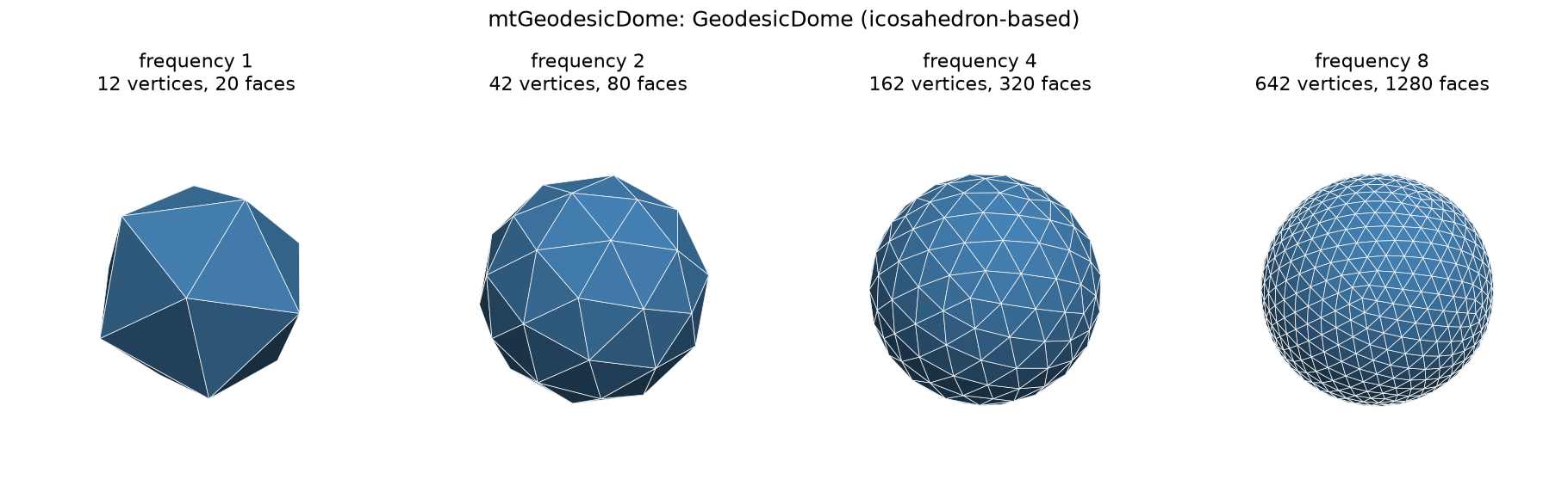
Project-URL: Documentation, https://github.com/takatsuka/GeodesicDome/blob/main/docs/index.md
|
|
12
|
+
Project-URL: Changelog, https://github.com/takatsuka/GeodesicDome/blob/main/CHANGELOG.md
|
|
13
|
+
Project-URL: Paper, https://doi.org/10.1016/j.neunet.2006.05.021
|
|
14
|
+
Keywords: geodesic dome,geodesic sphere,icosahedron,tetrahedron,dodecahedron,spherical grid,icosphere,self-organizing map,spherical SOM,neighbour search,map projection,equal earth,mesh,gpu,cuda
|
|
15
|
+
Classifier: Development Status :: 4 - Beta
|
|
16
|
+
Classifier: Intended Audience :: Science/Research
|
|
17
|
+
Classifier: Intended Audience :: Developers
|
|
18
|
+
Classifier: Operating System :: OS Independent
|
|
19
|
+
Classifier: Programming Language :: Python :: 3
|
|
20
|
+
Classifier: Programming Language :: Python :: 3 :: Only
|
|
21
|
+
Classifier: Programming Language :: Python :: 3.10
|
|
22
|
+
Classifier: Programming Language :: Python :: 3.11
|
|
23
|
+
Classifier: Programming Language :: Python :: 3.12
|
|
24
|
+
Classifier: Programming Language :: Python :: 3.13
|
|
25
|
+
Classifier: Programming Language :: Python :: 3.14
|
|
26
|
+
Classifier: Topic :: Scientific/Engineering :: Mathematics
|
|
27
|
+
Classifier: Topic :: Scientific/Engineering :: Artificial Intelligence
|
|
28
|
+
Classifier: Topic :: Scientific/Engineering :: Visualization
|
|
29
|
+
Classifier: Typing :: Typed
|
|
30
|
+
Requires-Python: >=3.10
|
|
31
|
+
Description-Content-Type: text/markdown
|
|
32
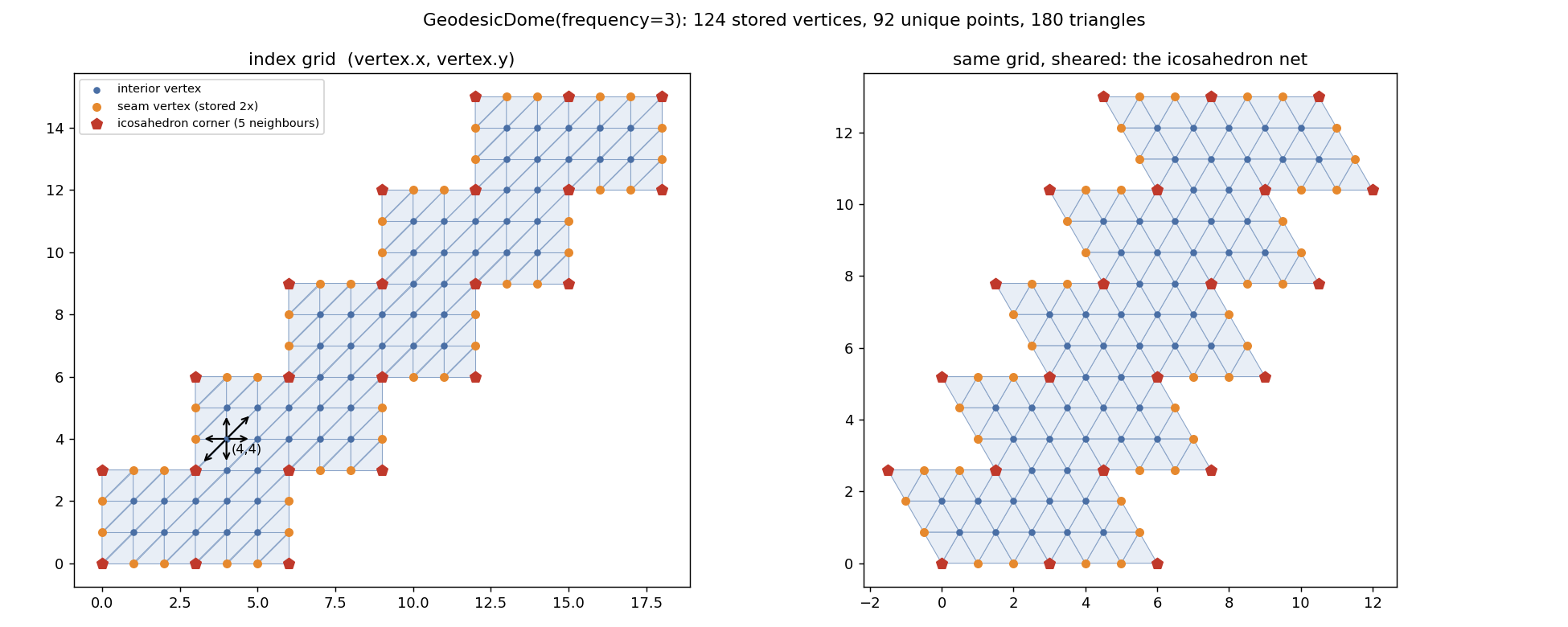
|
+
License-File: LICENSE
|
|
33
|
+
License-File: NOTICE
|
|
34
|
+
Requires-Dist: numpy>=1.23
|
|
35
|
+
Provides-Extra: interactive
|
|
36
|
+
Requires-Dist: matplotlib>=3.6; extra == "interactive"
|
|
37
|
+
Provides-Extra: gpu
|
|
38
|
+
Requires-Dist: torch>=2.1; extra == "gpu"
|
|
39
|
+
Provides-Extra: examples
|
|
40
|
+
Requires-Dist: matplotlib>=3.6; extra == "examples"
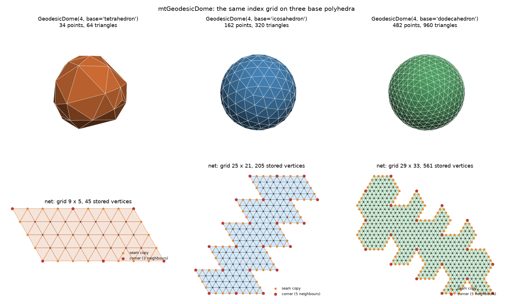
|
|
41
|
+
Requires-Dist: pillow; extra == "examples"
|
|
42
|
+
Provides-Extra: notebooks
|
|
43
|
+
Requires-Dist: matplotlib>=3.6; extra == "notebooks"
|
|
44
|
+
Requires-Dist: pillow; extra == "notebooks"
|
|
45
|
+
Requires-Dist: jupyterlab; extra == "notebooks"
|
|
46
|
+
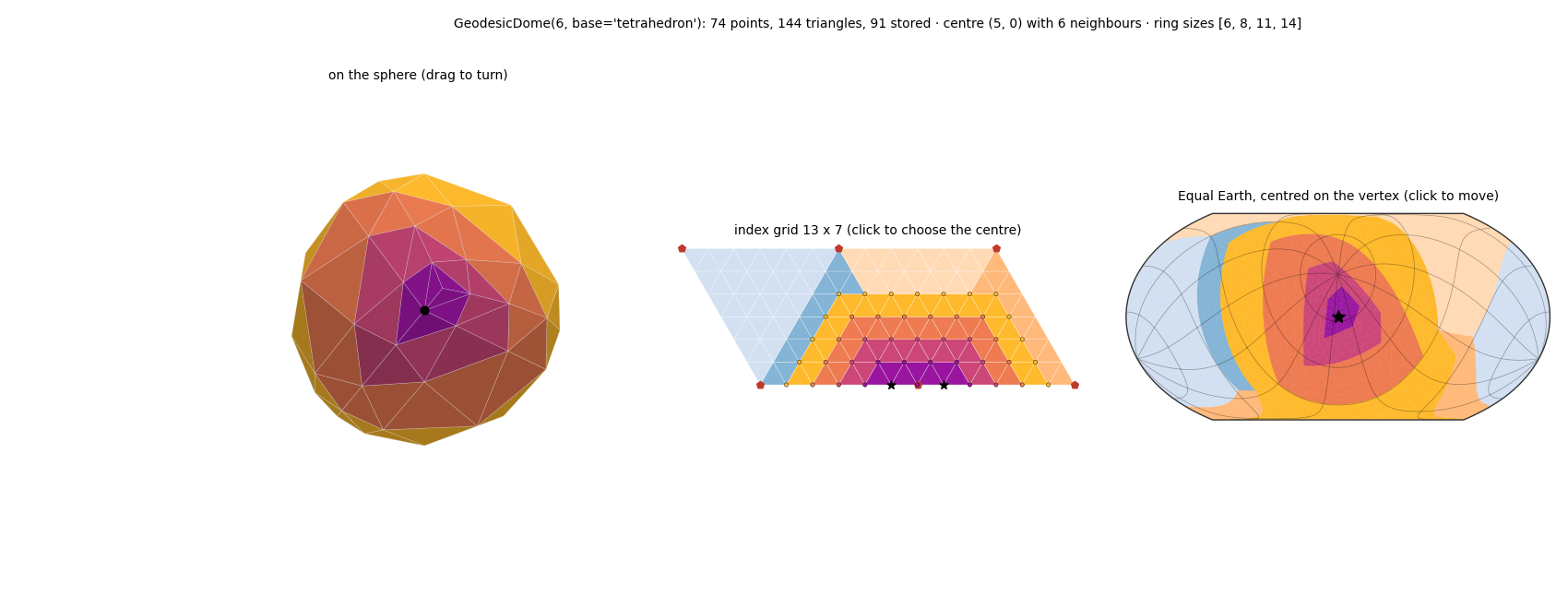
Requires-Dist: ipywidgets>=8; extra == "notebooks"
|
|
47
|
+
Requires-Dist: ipympl; extra == "notebooks"
|
|
48
|
+
Provides-Extra: legacy
|
|
49
|
+
Requires-Dist: plotly; extra == "legacy"
|
|
50
|
+
Requires-Dist: dash; extra == "legacy"
|
|
51
|
+
Provides-Extra: dev
|
|
52
|
+
Requires-Dist: matplotlib>=3.6; extra == "dev"
|
|
53
|
+
Requires-Dist: pytest>=7; extra == "dev"
|
|
54
|
+
Requires-Dist: pytest-cov; extra == "dev"
|
|
55
|
+
Requires-Dist: ruff<0.17,>=0.16; extra == "dev"
|
|
56
|
+
Requires-Dist: build; extra == "dev"
|
|
57
|
+
Requires-Dist: twine; extra == "dev"
|
|
58
|
+
Provides-Extra: all
|
|
59
|
+
Requires-Dist: matplotlib>=3.6; extra == "all"
|
|
60
|
+
Requires-Dist: pillow; extra == "all"
|
|
61
|
+
Requires-Dist: jupyterlab; extra == "all"
|
|
62
|
+
Requires-Dist: ipywidgets>=8; extra == "all"
|
|
63
|
+
Requires-Dist: ipympl; extra == "all"
|
|
64
|
+
Requires-Dist: plotly; extra == "all"
|
|
65
|
+
Requires-Dist: dash; extra == "all"
|
|
66
|
+
Requires-Dist: pytest>=7; extra == "all"
|
|
67
|
+
Requires-Dist: pytest-cov; extra == "all"
|
|
68
|
+
Requires-Dist: ruff<0.17,>=0.16; extra == "all"
|
|
69
|
+
Requires-Dist: build; extra == "all"
|
|
70
|
+
Requires-Dist: twine; extra == "all"
|
|
71
|
+
Dynamic: license-file
|
|
72
|
+
|
|
73
|
+
# GeodesicDome — geodesic domes and grids for Python
|
|
74
|
+
|
|
75
|
+
[](https://pypi.org/project/geodesicdomes/)
|
|
76
|
+
[](https://pypi.org/project/geodesicdomes/)
|
|
77
|
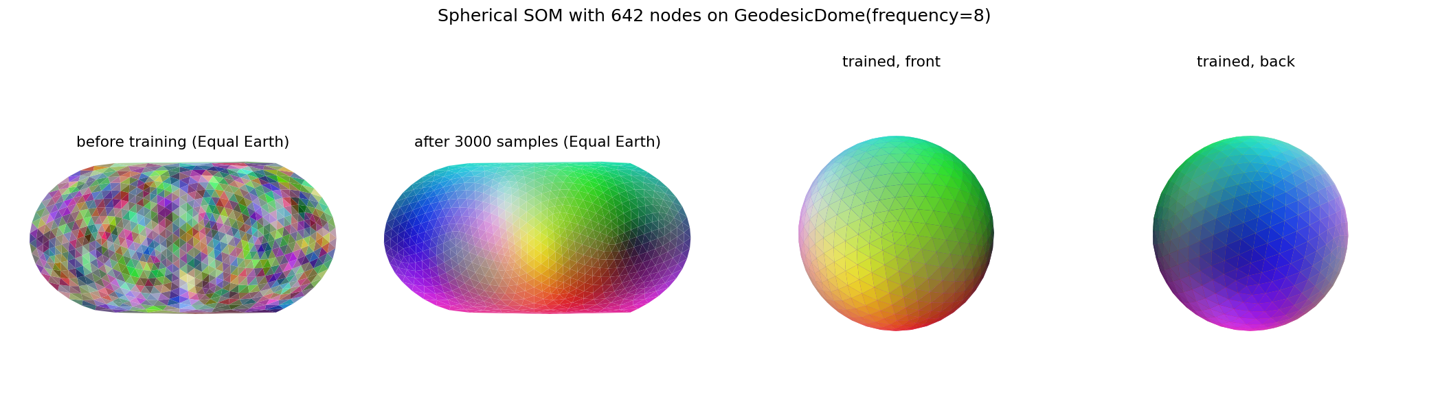
+
[](https://github.com/takatsuka/GeodesicDome/actions/workflows/tests.yml)
|
|
78
|
+
[](https://github.com/takatsuka/GeodesicDome/blob/main/LICENSE)
|
|
79
|
+
|
|
80
|
+
`mt.geodesicdome` builds **geodesic spheres** (domes of any frequency on an icosahedron, tetrahedron or dodecahedron) and
|
|
81
|
+
**flat hexagonal/rectilinear grids**, with fast neighbour search on both. It was written as the
|
|
82
|
+
lattice layer for Self-Organising Maps (SOMs), but it works just as well for meshing,
|
|
83
|
+
sampling points evenly on a sphere, or cellular automata on a globe.
|
|
84
|
+
|
|
85
|
+
| What | Name |
|
|
86
|
+
|---|---|
|
|
87
|
+
| `pip install …` | `geodesicdomes` |
|
|
88
|
+
| Python import | `mt.geodesicdome` (`mt` is a namespace package shared by future `mt.*` libraries) |
|
|
89
|
+
| Repository | [`takatsuka/GeodesicDome`](https://github.com/takatsuka/GeodesicDome) |
|
|
90
|
+
|
|
91
|
+
|
|
92
|
+
|
|
93
|
+
**What you get**
|
|
94
|
+
|
|
95
|
+
| Feature | Where |
|
|
96
|
+
|---|---|
|
|
97
|
+
| Geodesic dome of any frequency *f*: 10f²+2 points, 20f² triangles, all on the unit sphere | `mt.geodesicdome.grid.geodesicdome.GeodesicDome` |
|
|
98
|
+
| Other base solids: tetrahedron (4HSOM array, 2f²+2 points) and dodecahedron (30f²+2 points) | `GeodesicDome(f, base='tetrahedron' / 'dodecahedron')` |
|
|
99
|
+
| Neighbour search and *k*-ring neighbourhoods that continue across the seams of the net | `get_neighbours`, `get_neighbours_in_distance` |
|
|
100
|
+
| NumPy export of points and triangles (outward-facing winding) | `get_all_xyz`, `get_all_triangles` |
|
|
101
|
+
| A data payload per vertex, e.g. SOM weight vectors | `vertex.set_data(...)` / `vertex.data` |
|
|
102
|
+
| Four map projections to flatten the sphere | `mt.geodesicdome.projection` |
|
|
103
|
+
| **Interactive map: drag with the mouse to rotate the sphere inside the projection** | `mt.geodesicdome.interactive.ProjectionViewer` |
|
|
104
|
+
| Flat hexagonal or rectilinear grids, with borders or as a torus | `mt.geodesicdome.grid.plane.Plane` |
|
|
105
|
+
|
|
106
|
+
---
|
|
107
|
+
|
|
108
|
+
## 1. Installation
|
|
109
|
+
|
|
110
|
+
Requires Python ≥ 3.10 and NumPy. The interactive viewer and the examples also need matplotlib.
|
|
111
|
+
|
|
112
|
+
```bash
|
|
113
|
+
pip install geodesicdomes # the library (numpy only)
|
|
114
|
+
pip install "geodesicdomes[interactive]" # + matplotlib, for mt.geodesicdome.interactive
|
|
115
|
+
pip install "geodesicdomes[gpu]" # + torch, to use an NVIDIA (CUDA) or Apple Silicon (MPS) GPU
|
|
116
|
+
```
|
|
117
|
+
|
|
118
|
+
Check that it works:
|
|
119
|
+
|
|
120
|
+
```bash
|
|
121
|
+
python -c "from mt.geodesicdome.grid.geodesicdome import GeodesicDome; print(GeodesicDome(4))"
|
|
122
|
+
# GeodesicDome(frequency=4)
|
|
123
|
+
```
|
|
124
|
+
|
|
125
|
+
The examples, the tests and `setup_env.sh` are in the
|
|
126
|
+
[GitHub repository](https://github.com/takatsuka/GeodesicDome), not in the pip package.
|
|
127
|
+
|
|
128
|
+
### Working on this repository: `setup_env.sh` (recommended)
|
|
129
|
+
|
|
130
|
+
One command creates a virtual environment with everything the project uses: numpy, matplotlib, pillow,
|
|
131
|
+
plotly and dash for the older viewers, and pytest. It also installs this package in editable mode, so any
|
|
132
|
+
`.py` file in any folder of the project can `import mt.geodesicdome`.
|
|
133
|
+
|
|
134
|
+
```bash
|
|
135
|
+
cd GeodesicDome
|
|
136
|
+
./setup_env.sh # once
|
|
137
|
+
python examples/01_quickstart.py # works straight away, in the same terminal
|
|
138
|
+
python examples/09_interactive_projection.py
|
|
139
|
+
```
|
|
140
|
+
|
|
141
|
+
* **It leaves you in a ready shell.** When it finishes, it opens a shell in which the environment is active
|
|
142
|
+
(the prompt starts with `(GeodesicDome)`), so `python` is the project's Python. Type `exit` to return to
|
|
143
|
+
your previous shell. `--no-shell` skips this.
|
|
144
|
+
* **New terminals are ready too.** It adds a small block to `~/.zshrc` (and `~/.bashrc` if you have one) that
|
|
145
|
+
activates the environment whenever you are inside the project and deactivates it when you leave.
|
|
146
|
+
`--no-shell-hook` skips this; `./setup_env.sh --remove-shell-hook` removes it.
|
|
147
|
+
* **The environment lives in `~/.venvs/GeodesicDome`, outside the repository.** This repository sits in Google Drive,
|
|
148
|
+
which syncs every file of a virtual environment and can make them online-only, so imports hang or fail.
|
|
149
|
+
* **Anywhere else**, run `source ~/.venvs/GeodesicDome/bin/activate`, or call the environment's Python
|
|
150
|
+
directly: `~/.venvs/GeodesicDome/bin/python path/to/script.py`.
|
|
151
|
+
* **It is safe to re-run at any time.** A healthy environment is reused, and missing packages are added. A broken
|
|
152
|
+
one, for example after `brew upgrade python`, is rebuilt automatically.
|
|
153
|
+
* **It picks the newest Python ≥ 3.10 it can find.** Use `--python /opt/homebrew/bin/python3.13` to choose one.
|
|
154
|
+
* **It installs the GPU packages this machine can use.** PyTorch with MPS on Apple Silicon; on Linux/Windows with an
|
|
155
|
+
NVIDIA GPU, PyTorch built for the CUDA version the driver supports (read from `nvidia-smi`) plus the matching CuPy;
|
|
156
|
+
PyTorch for ROCm on an AMD GPU. Without a GPU nothing extra is installed and computations use every CPU core. The
|
|
157
|
+
last step checks that the GPU really works. `--gpu torch|cupy|none` narrows or skips this, and
|
|
158
|
+
`--torch-index cu126` (or a URL) overrides the PyTorch wheel index.
|
|
159
|
+
* **Other options:** `--recreate` builds from scratch, `--check` only verifies, `--minimal` installs numpy only
|
|
160
|
+
(and no GPU packages), and `--no-legacy` skips plotly and dash. See `./setup_env.sh --help`.
|
|
161
|
+
* **IDE:** in PyCharm or VS Code, choose `~/.venvs/GeodesicDome/bin/python` as the project interpreter.
|
|
162
|
+
|
|
163
|
+
### Other ways to install
|
|
164
|
+
|
|
165
|
+
```bash
|
|
166
|
+
pip install "git+https://github.com/takatsuka/GeodesicDome.git" # latest development version
|
|
167
|
+
pip install -e ".[interactive]" # from a local checkout, editable
|
|
168
|
+
```
|
|
169
|
+
|
|
170
|
+
Optional extras: `interactive` (matplotlib), `examples` (+ pillow), `legacy` (plotly and dash, for the old
|
|
171
|
+
viewer scripts), `dev` (pytest, ruff, build, twine), and `all`.
|
|
172
|
+
|
|
173
|
+
---
|
|
174
|
+
|
|
175
|
+
## 2. Quick start
|
|
176
|
+
|
|
177
|
+
```python
|
|
178
|
+
import numpy as np
|
|
179
|
+
from mt.geodesicdome.grid.geodesicdome import GeodesicDome
|
|
180
|
+
|
|
181
|
+
dome = GeodesicDome(frequency=8) # icosahedron with each edge cut into 8
|
|
182
|
+
|
|
183
|
+
xyz = dome.get_all_xyz() # (N, 3) unit vectors
|
|
184
|
+
tri = dome.get_all_triangles().reshape(-1, 3) # (20 f², 3) indices into xyz
|
|
185
|
+
print(xyz.shape, tri.shape) # (729, 3) (1280, 3)
|
|
186
|
+
|
|
187
|
+
# neighbours of a vertex, addressed by its (x, y) position on the index grid
|
|
188
|
+
v = dome.get_vertex_at(12, 14)
|
|
189
|
+
dome.unmark_vertices() # always reset before a search
|
|
190
|
+
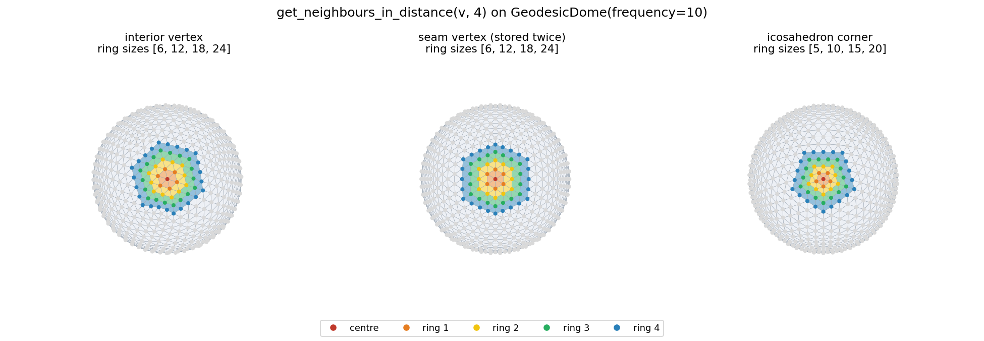
ring1 = dome.get_neighbours(v, False) # 6 neighbours (5 at the 12 corners)
|
|
191
|
+
|
|
192
|
+
dome.unmark_vertices()
|
|
193
|
+
rings = dome.get_neighbours_in_distance(v, 3) # [[ring 1], [ring 2], [ring 3]]
|
|
194
|
+
print([len(r) for r in rings]) # [6, 12, 18]
|
|
195
|
+
|
|
196
|
+
v.set_data(np.zeros(3)) # attach anything to a vertex
|
|
197
|
+
```
|
|
198
|
+
|
|
199
|
+
You can also refine step by step. `split` multiplies the frequency, so
|
|
200
|
+
`GeodesicDome(2).split(3)` gives frequency 6.
|
|
201
|
+
|
|
202
|
+
---
|
|
203
|
+
|
|
204
|
+
## 3. Core concepts
|
|
205
|
+
|
|
206
|
+
### 3.1 Frequency
|
|
207
|
+
|
|
208
|
+
| frequency *f* | unique points 10f²+2 | triangles 20f² | stored vertices | mean edge (unit sphere) |
|
|
209
|
+
|---:|---:|---:|---:|---:|
|
|
210
|
+
| 1 | 12 | 20 | 22 | 1.052 |
|
|
211
|
+
| 2 | 42 | 80 | 63 | 0.582 |
|
|
212
|
+
| 4 | 162 | 320 | 205 | 0.298 |
|
|
213
|
+
| 8 | 642 | 1 280 | 729 | 0.150 |
|
|
214
|
+
| 12 | 1 442 | 2 880 | 1 573 | 0.100 |
|
|
215
|
+
|
|
216
|
+
Every point has 6 neighbours, except the 12 original icosahedron corners, which have 5.
|
|
217
|
+
Rings near a corner are therefore slightly smaller (for example 5, 10, 15 around a corner itself).
|
|
218
|
+
|
|
219
|
+
### 3.2 The unfolded net and seam vertices
|
|
220
|
+
|
|
221
|
+
Internally, the icosahedron is unfolded onto an integer grid. Each vertex has a grid position
|
|
222
|
+
`(vertex.x, vertex.y)`, and its neighbours on the sphere are always the six grid offsets
|
|
223
|
+
`(±1, 0)`, `(0, ±1)`, `(+1, +1)` and `(−1, −1)`. That is what makes neighbour look-ups fast.
|
|
224
|
+
|
|
225
|
+
This indexed geodesic data structure was introduced for the spherical self-organising map in:
|
|
226
|
+
|
|
227
|
+
> Y. Wu and M. Takatsuka, "Spherical self-organizing map using efficient indexed geodesic data structure,"
|
|
228
|
+
> *Neural Networks*, vol. 19, no. 6–7, pp. 900–910, 2006. [doi:10.1016/j.neunet.2006.05.021](https://doi.org/10.1016/j.neunet.2006.05.021)
|
|
229
|
+
|
|
230
|
+
```bibtex
|
|
231
|
+
@article{wu2006spherical,
|
|
232
|
+
author = {Wu, Yingxin and Takatsuka, Masahiro},
|
|
233
|
+
title = {Spherical self-organizing map using efficient indexed geodesic data structure},
|
|
234
|
+
journal = {Neural Networks},
|
|
235
|
+
volume = {19},
|
|
236
|
+
number = {6--7},
|
|
237
|
+
pages = {900--910},
|
|
238
|
+
year = {2006},
|
|
239
|
+
month = {07},
|
|
240
|
+
doi = {10.1016/j.neunet.2006.05.021}
|
|
241
|
+
}
|
|
242
|
+
```
|
|
243
|
+
|
|
244
|
+
|
|
245
|
+
|
|
246
|
+
To fold the net back into a sphere, points on its border are **stored more than once**, and each copy
|
|
247
|
+
lists the others in `vertex.same_vertices`. As a result:
|
|
248
|
+
|
|
249
|
+
* `get_all_vertices()` / `get_all_xyz()` return **N ≥ 10f²+2** entries (for example 729 instead of 642 at f = 8).
|
|
250
|
+
* Neighbour searches already handle the copies, so rings continue across seams and never
|
|
251
|
+
contain the same point twice.
|
|
252
|
+
* To get a clean mesh with each point exactly once, de-duplicate by position.
|
|
253
|
+
`examples/dome_utils.py` has a ready-made `unique_mesh(dome)` that returns
|
|
254
|
+
`(points, faces, index_map)`.
|
|
255
|
+
|
|
256
|
+
### 3.3 The `visited` flag
|
|
257
|
+
|
|
258
|
+
The neighbour searches mark vertices with `vertex.visited = True` so they are not returned twice.
|
|
259
|
+
**Call `dome.unmark_vertices()` before every new query**. Otherwise vertices from the previous
|
|
260
|
+
query will be missing from the result.
|
|
261
|
+
|
|
262
|
+
### 3.4 Coordinates
|
|
263
|
+
|
|
264
|
+
* `vertex.coord` is the unit vector (x, y, z). The dome is built with its poles on the **±y** axis.
|
|
265
|
+
* `vertex.latlon_coord` is `(colatitude from +y, longitude)` in radians.
|
|
266
|
+
* `vertex.id` is the row of the vertex in `get_all_xyz()`. It is assigned when faces are built
|
|
267
|
+
(`get_faces()` / `get_all_triangles()`), so call one of those first.
|
|
268
|
+
* The map projections use **+z** as their north pole (`latitude = arcsin(z)`).
|
|
269
|
+
|
|
270
|
+
### 3.5 Base polyhedra: tetrahedron, icosahedron, dodecahedron
|
|
271
|
+
|
|
272
|
+
The icosahedron is the default. `base=` builds the dome on another solid, with the same index grid, the same
|
|
273
|
+
six neighbour offsets and the same API:
|
|
274
|
+
|
|
275
|
+
```python
|
|
276
|
+
GeodesicDome(8) # icosahedron: 642 points (10f²+2)
|
|
277
|
+
GeodesicDome(8, base='tetrahedron') # tetrahedron: 130 points ( 2f²+2)
|
|
278
|
+
GeodesicDome(8, base='dodecahedron') # dodecahedron: 1922 points (30f²+2)
|
|
279
|
+
```
|
|
280
|
+
|
|
281
|
+
`base` takes `'icosahedron'` / `'icosa'`, `'tetrahedron'` / `'tetra'`, `'dodecahedron'` / `'dodeca'` (any case).
|
|
282
|
+
`GeodesicDome(...)` then returns an `IcosahedronDome`, `TetrahedronDome` or `DodecahedronDome`, all subclasses
|
|
283
|
+
of `GeodesicDome`; `dome.base` says which.
|
|
284
|
+
|
|
285
|
+
| base | unique points | triangles | stored vertices (grid) | corners | net |
|
|
286
|
+
|---|---:|---:|---|---|---|
|
|
287
|
+
| `'tetrahedron'` | 2f²+2 | 4f² | (f+1)(2f+1): an `(f+1) × (2f+1)` array, every cell used | 4, with 3 neighbours | the 4HSOM orthogonal array of de Sousa & Oliveira (2012) |
|
|
288
|
+
| `'icosahedron'` | 10f²+2 | 20f² | 729 at f = 8 | 12, with 5 neighbours | the 5-strip net of Wu & Takatsuka (2006) |
|
|
289
|
+
| `'dodecahedron'` | 30f²+2 | 60f² | 2 081 at f = 8 | 12 pentagon centres, with 5 neighbours | the pentakis dodecahedron on the strip net, cut along pentagon edges |
|
|
290
|
+
|
|
291
|
+
* **Tetrahedron.** Following de Sousa & Oliveira's 4HSOM, the four faces form a parallelogram stored as
|
|
292
|
+
`f + 1` rows (`y = 0..f`) by `2f + 1` columns (`x = 0..2f`). Column `0` and column `2f` are the same points,
|
|
293
|
+
and the bottom and top rows fold about their middle points: `(i, 0) = (2f − i, 0)` and `(i, f) = (2f − i, f)`.
|
|
294
|
+
The four corners are A at `(0, 0)`/`(2f, 0)`, B at `(f, 0)`, C at `(0, f)`/`(2f, f)` and D, the north
|
|
295
|
+
pole, at `(f, f)`. Its cells vary much more in area than the icosahedron's.
|
|
296
|
+
* **Dodecahedron.** Each pentagon is cut into 5 triangles meeting at its centre (the pentakis dodecahedron) and
|
|
297
|
+
each triangle into an *f*-frequency grid on the flat pentagon. Frequency 1 has 32 points: the 20 dodecahedron
|
|
298
|
+
corners (6 neighbours) and the 12 pentagon centres (5 neighbours), which point the same way as the
|
|
299
|
+
icosahedron's corners.
|
|
300
|
+
|
|
301
|
+
For these two solids the net has notches, so each vertex also stores a 6-bit `neighbour_mask` of the grid
|
|
302
|
+
offsets that are real edges; the search is still pure index arithmetic. The nets themselves are in
|
|
303
|
+
`mt.geodesicdome.grid.polyhedra` (`base_net(name)`).
|
|
304
|
+
|
|
305
|
+
|
|
306
|
+
|
|
307
|
+
**Explore them interactively.** `examples/11_interactive_base_polyhedra.py` (and the notebook of the same name)
|
|
308
|
+
shows one dome three ways at once: on the sphere, on its index grid and in a map projection centred on a
|
|
309
|
+
vertex. The vertex's neighbour rings are highlighted in all three, so you can see a neighbourhood
|
|
310
|
+
that is compact on the sphere split across the seams of the net. Click the net or the map to move it.
|
|
311
|
+
It can also colour every cell by its spherical area; compare the tetrahedron with the other two.
|
|
312
|
+
`ProjectionViewer(dome, colors='base')` colours any dome by the faces of its own base solid.
|
|
313
|
+
|
|
314
|
+
|
|
315
|
+
|
|
316
|
+
---
|
|
317
|
+
|
|
318
|
+
## 4. API reference
|
|
319
|
+
|
|
320
|
+
### `GeodesicDome(frequency=1, base='icosahedron')` — `mt.geodesicdome.grid.geodesicdome`
|
|
321
|
+
|
|
322
|
+
| Member | Description |
|
|
323
|
+
|---|---|
|
|
324
|
+
| `base` | `'icosahedron'`, `'tetrahedron'` or `'dodecahedron'` |
|
|
325
|
+
| `frequency`, `x_max`, `y_max` | current frequency and the extent of the index grid |
|
|
326
|
+
| `split(n)` | subdivide every edge into `n` more segments (frequency ×= n) |
|
|
327
|
+
| `get_all_vertices()` | list of `GeodesicVertex`, including seam copies |
|
|
328
|
+
| `get_vertex_at(x, y)` | vertex at a grid position, or `None` |
|
|
329
|
+
| `get_faces()` | flat list of vertices, 3 per triangle (also assigns `vertex.id`) |
|
|
330
|
+
| `get_all_triangles()` | flat `ndarray` of vertex ids; `.reshape(-1, 3)` gives the triangles |
|
|
331
|
+
| `get_all_xyz()` | `(N, 3)` array of coordinates, row = `vertex.id` |
|
|
332
|
+
| `get_number_of_vertices_per_face()` | `3` |
|
|
333
|
+
| `get_neighbours(v, False)` | immediate neighbours of `v` |
|
|
334
|
+
| `get_neighbours_in_distance(v, d)` | list of `d` rings: `[[ring 1], [ring 2], ...]` |
|
|
335
|
+
| `unmark_vertices()` | reset every `visited` flag (do this before each search) |
|
|
336
|
+
|
|
337
|
+
### `GeodesicVertex`
|
|
338
|
+
|
|
339
|
+
`x`, `y` (grid position) · `coord` (xyz) · `latlon_coord` · `id` · `same_vertices` (seam copies or `None`) ·
|
|
340
|
+
`data` / `set_data(obj)` · `visited` · `projected_coord` (set by a projection).
|
|
341
|
+
|
|
342
|
+
### Projections — `mt.geodesicdome.projection`
|
|
343
|
+
|
|
344
|
+
| Class | Module |
|
|
345
|
+
|---|---|
|
|
346
|
+
| `KavrayskiyVII` | `kavrayskiy` |
|
|
347
|
+
| `WagnerVI`, `WagnerIII` | `wagner` |
|
|
348
|
+
| `EqualEarth` | `equal_earth` |
|
|
349
|
+
|
|
350
|
+
```python
|
|
351
|
+
from mt.geodesicdome.projection.equal_earth import EqualEarth
|
|
352
|
+
tri2d = EqualEarth().build(dome) # (M, 3) triangle ids; sets v.projected_coord
|
|
353
|
+
xy = [v.projected_coord for v in dome.get_all_vertices()]
|
|
354
|
+
EqualEarth().xyz_to_2d(np.array([0, 0, 1])) # project a single point
|
|
355
|
+
```
|
|
356
|
+
|
|
357
|
+
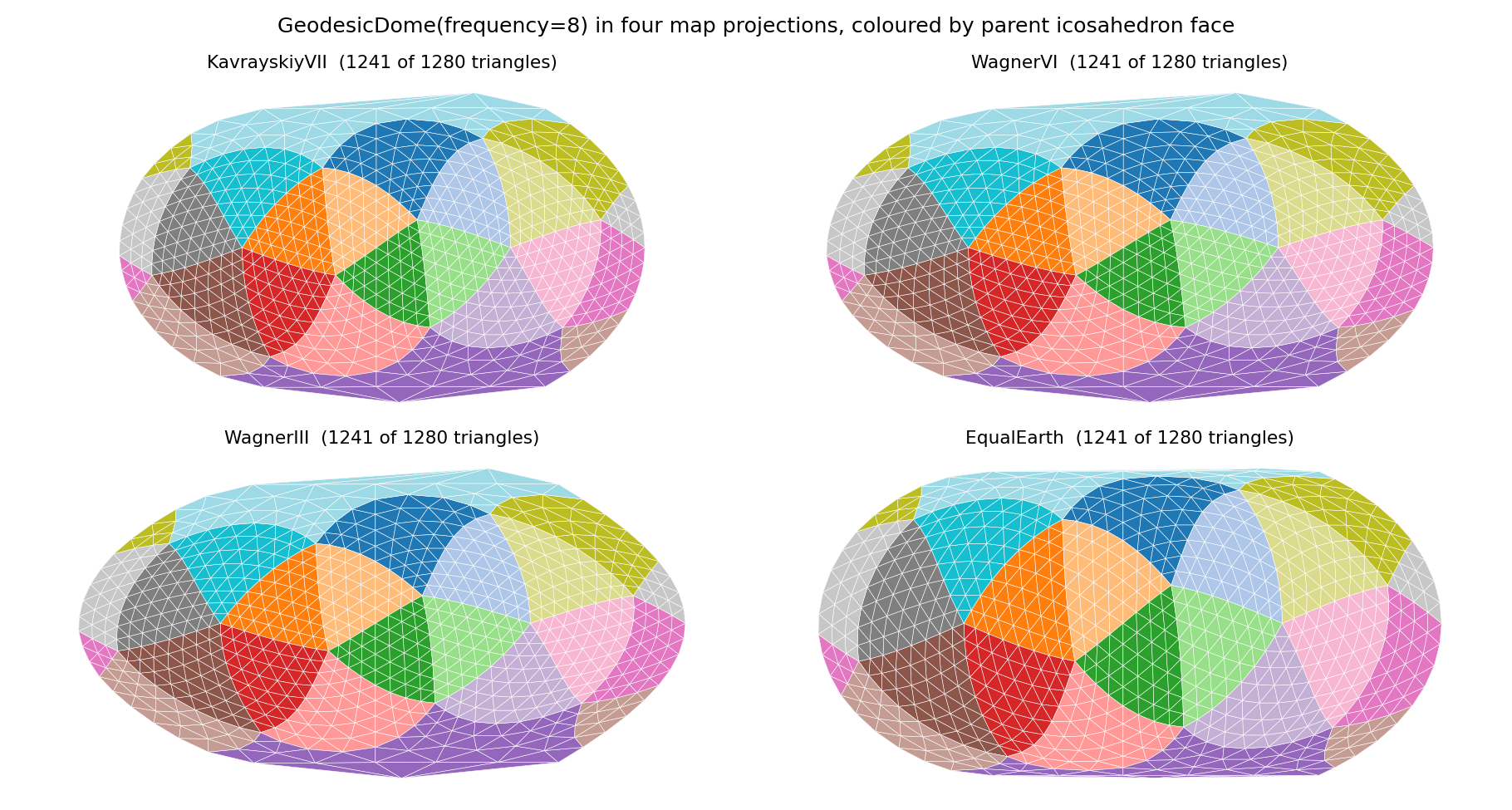
`build` leaves out the few triangles that would wrap across the ±180° meridian, so M < 20f².
|
|
358
|
+
For a complete map, with no missing triangles and any orientation of the sphere, use
|
|
359
|
+
`mt.geodesicdome.interactive` (below).
|
|
360
|
+
|
|
361
|
+
Vectorised helpers on every projection: `latlong_to_2d(lat, lon)` (arrays, radians),
|
|
362
|
+
`xyz_to_2d_many(xyz)` for an `(N, 3)` array, and `outline()`, the map boundary as a polygon.
|
|
363
|
+
|
|
364
|
+
|
|
365
|
+
|
|
366
|
+
### Interactive projection — `mt.geodesicdome.interactive`
|
|
367
|
+
|
|
368
|
+
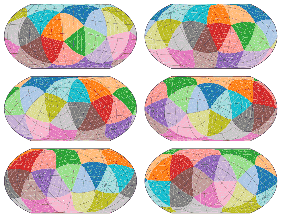
`ProjectionViewer` shows the dome in a map projection that you can rotate. **Click and drag on the map, and the
|
|
369
|
+
sphere turns underneath it**: dragging left or right spins it about the map's polar axis, and dragging up or down
|
|
370
|
+
tilts it. The projection is recomputed on every mouse move.
|
|
371
|
+
|
|
372
|
+
```python
|
|
373
|
+
from mt.geodesicdome.grid.geodesicdome import GeodesicDome
|
|
374
|
+
from mt.geodesicdome.interactive import ProjectionViewer
|
|
375
|
+
|
|
376
|
+
viewer = ProjectionViewer(GeodesicDome(8), 'Equal Earth')
|
|
377
|
+
viewer.show()
|
|
378
|
+
```
|
|
379
|
+
|
|
380
|
+
|
|
381
|
+
|
|
382
|
+
| Mouse / key | Action |
|
|
383
|
+
|---|---|
|
|
384
|
+
| drag (left button) | rotate the sphere (a fast preview is drawn while dragging; full quality returns on release) |
|
|
385
|
+
| arrow keys | rotate by 5° (with shift: 1°) |
|
|
386
|
+
| `,` / `.` | roll the view about the map centre |
|
|
387
|
+
| `r` / *Reset view* button | back to the starting view |
|
|
388
|
+
| `p` / radio buttons | switch projection: Equal Earth, Kavrayskiy VII, Wagner VI, Wagner III |
|
|
389
|
+
| `g` / `e` | show or hide the graticule / the triangle edges |
|
|
390
|
+
|
|
391
|
+
The black graticule shows the latitude and longitude lines *of the original sphere*, so you can see how it has
|
|
392
|
+
turned. The status line gives the original point now at the map centre.
|
|
393
|
+
|
|
394
|
+
**Options and methods**
|
|
395
|
+
|
|
396
|
+
```python
|
|
397
|
+
viewer = ProjectionViewer(
|
|
398
|
+
dome, 'Wagner VI',
|
|
399
|
+
colors='position', # 'position' (default), 'base' (faces of the dome's base solid), 'icosahedron',
|
|
400
|
+
# 'data' (vertex.data), a colour name,
|
|
401
|
+
# or an array per stored vertex / per unique point / per face
|
|
402
|
+
cmap='viridis', # used when colors holds scalars (a colour bar is added)
|
|
403
|
+
edges=None, # triangle edges; default: on for frequency <= 12
|
|
404
|
+
graticule=True,
|
|
405
|
+
view=(-33.9, 151.2), # (lat, lon) in degrees of the original point to put at the centre
|
|
406
|
+
)
|
|
407
|
+
viewer.rotate(d_lon=30, d_lat=-10, roll=0) # degrees, same axes as dragging
|
|
408
|
+
viewer.set_view(lat, lon) # centre the map on an original point
|
|
409
|
+
viewer.set_rotation(R) # any 3x3 rotation matrix (original -> view)
|
|
410
|
+
viewer.set_projection('Kavrayskiy VII')
|
|
411
|
+
viewer.set_colors(values, vmin=0, vmax=1)
|
|
412
|
+
viewer.on_rotate(lambda v: print(v.centre)) # called after every change of the view
|
|
413
|
+
viewer.save('map.png')
|
|
414
|
+
```
|
|
415
|
+
|
|
416
|
+
Colouring by `vertex.data` means a trained spherical SOM (see `examples/06_spherical_som.py`) can be explored
|
|
417
|
+
directly: store each node's weight vector as an RGB colour with `set_data` and pass `colors='data'`.
|
|
418
|
+
|
|
419
|
+
**Running it.** It needs a matplotlib GUI backend. `python examples/09_interactive_projection.py` from a desktop
|
|
420
|
+
terminal or IDE opens a window. In Jupyter, run `%matplotlib widget` first (`pip install ipympl`).
|
|
421
|
+
|
|
422
|
+
**How it works.** `SphereMap` (numpy only) rotates the de-duplicated mesh and projects it. Unlike
|
|
423
|
+
`Projection.build`, it keeps every triangle:
|
|
424
|
+
* a triangle that straddles the ±180° meridian is drawn twice, shifted by ±360° of longitude, and clipped to the
|
|
425
|
+
map outline;
|
|
426
|
+
* the triangle that contains a pole becomes a polygon running along the pole line;
|
|
427
|
+
* exact alignments, such as a pole lying precisely on an edge in the un-rotated view, are broken by a fixed
|
|
428
|
+
10⁻⁶ rad rotation that is invisible on screen.
|
|
429
|
+
|
|
430
|
+
The tests (`tests/test_interactive.py`) render random and deliberately degenerate orientations in all four
|
|
431
|
+
projections and check that no pixel inside the map is left uncovered. `SphereMap.polygons(R)` is also usable on
|
|
432
|
+
its own, for example to draw a rotated map in your own figure.
|
|
433
|
+
|
|
434
|
+
### Compute backends: GPU or all CPU cores — `mt.geodesicdome.backend`, `mt.geodesicdome.compute`
|
|
435
|
+
|
|
436
|
+
Heavy array work runs on a GPU when one is available and otherwise on every CPU core. Nothing extra is required:
|
|
437
|
+
with numpy alone you get the multi-threaded CPU backend; install torch (`pip install "geodesicdomes[gpu]"`) for an
|
|
438
|
+
NVIDIA GPU (CUDA) or the Apple Silicon GPU (MPS), or CuPy for CUDA.
|
|
439
|
+
|
|
440
|
+
```python
|
|
441
|
+
from mt.geodesicdome import backend, compute
|
|
442
|
+
from mt.geodesicdome.grid.geodesicdome import GeodesicDome
|
|
443
|
+
|
|
444
|
+
print(backend.describe()) # what is available, and the default
|
|
445
|
+
b = backend.get_backend() # auto: CUDA -> CuPy -> MPS -> NumPy on all cores
|
|
446
|
+
mesh = compute.DomeArrays.from_dome(GeodesicDome(32))
|
|
447
|
+
rings = compute.ring_distance(mesh) # (10242, 10242) distances in neighbour spacings
|
|
448
|
+
idx = compute.nearest_vertex(mesh.points, queries) # nearest dome vertex of each query direction
|
|
449
|
+
```
|
|
450
|
+
|
|
451
|
+
| Choose | How |
|
|
452
|
+
|---|---|
|
|
453
|
+
| a device | `get_backend('cuda')`, `'cuda:1'`, `'mps'`, `'cupy'`, `'cpu'`/`'numpy'`, `'torch:cpu'`; or pass `backend=` to any function |
|
|
454
|
+
| the default | `backend.set_default_backend('cpu')` or `MTGEODESIC_BACKEND=cpu` |
|
|
455
|
+
| CPU threads | `MTGEODESIC_NUM_THREADS=8` (default: every core) |
|
|
456
|
+
| GPU precision | `MTGEODESIC_DTYPE=float64` (default float32 on a GPU; the Apple GPU is float32 only; the CPU always uses float64) |
|
|
457
|
+
| block size | `MTGEODESIC_MEMORY=512MB` (default: from the free device memory) |
|
|
458
|
+
|
|
459
|
+
A `Backend` offers the few array operations the geodesic libraries need with the same meaning on numpy, cupy and
|
|
460
|
+
torch arrays, plus `block_rows()`/`map_blocks()` to cut work into blocks that fit in memory and run them on all CPU
|
|
461
|
+
cores. mtGeodesicSOM trains on it.
|
|
462
|
+
|
|
463
|
+
### `Plane(x, y, lattice, topology)` — `mt.geodesicdome.grid.plane`
|
|
464
|
+
|
|
465
|
+
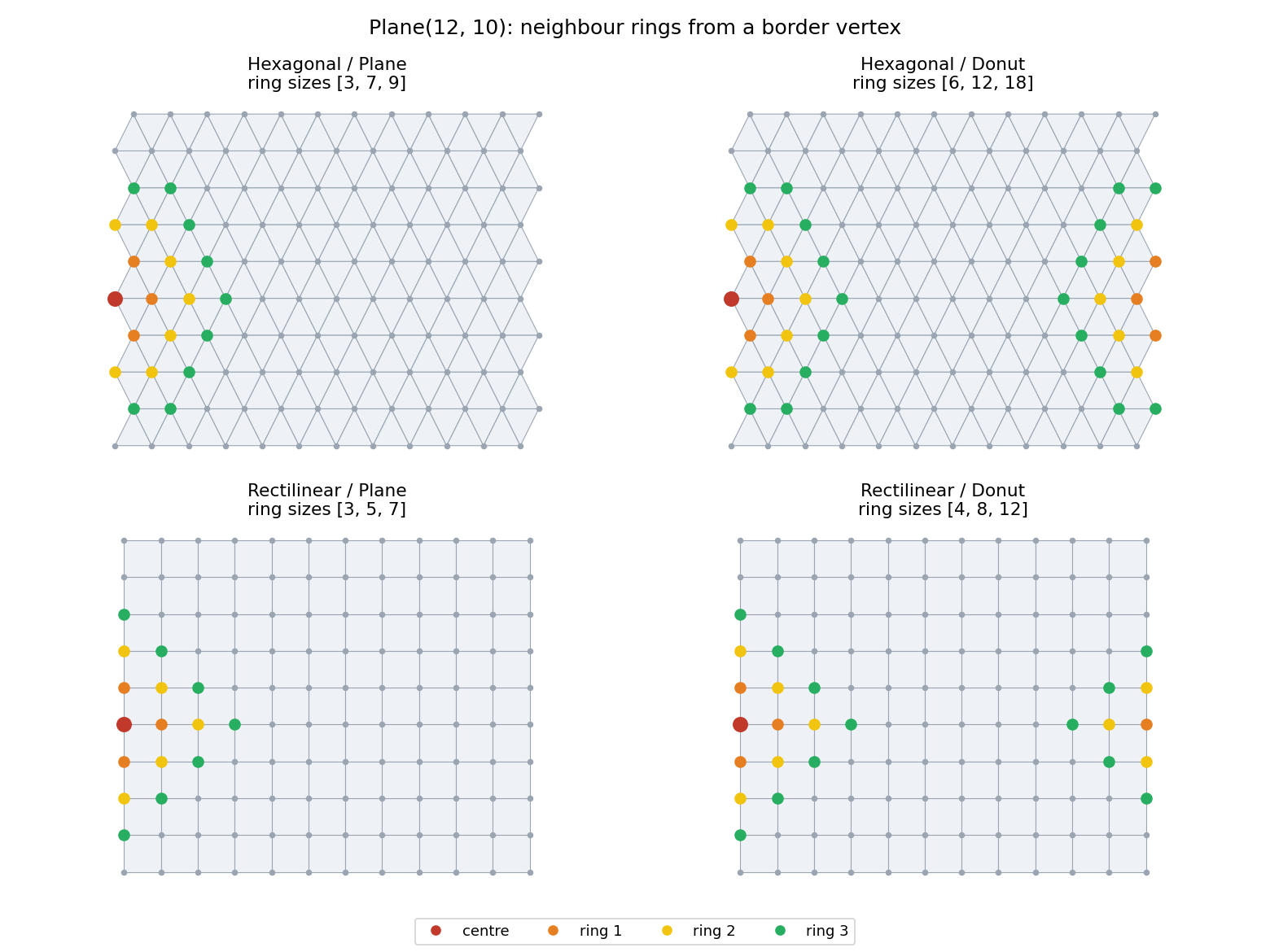
* `lattice`: `Lattice.Hexagonal` (6 neighbours, odd rows shifted by ½) or `Lattice.Rectilinear` (4 neighbours).
|
|
466
|
+
* `topology`: `Topology.Plane` (hard borders) or `Topology.Donut` (wraps around like a torus). Use an even
|
|
467
|
+
height with a hexagonal donut. Faces are not generated across the wrap.
|
|
468
|
+
* It has the same `Manifold` interface as the dome: `get_vertex_at`, `get_neighbours`,
|
|
469
|
+
`get_neighbours_in_distance`, `get_faces` (3 or 4 vertices per face), `get_all_xyz`, `get_all_triangles`, `unmark_vertices`.
|
|
470
|
+
|
|
471
|
+
Because both classes share the `Manifold` interface, code such as a SOM can switch between a flat
|
|
472
|
+
map, a torus and a sphere without changes.
|
|
473
|
+
|
|
474
|
+
|
|
475
|
+
|
|
476
|
+
---
|
|
477
|
+
|
|
478
|
+
## 5. Examples
|
|
479
|
+
|
|
480
|
+
Run them from the repository root, e.g. `python examples/04_neighbours.py`. They work straight
|
|
481
|
+
from a checkout without installing, and their images and files go to `examples/output/`.
|
|
482
|
+
|
|
483
|
+
| Script | Shows |
|
|
484
|
+
|---|---|
|
|
485
|
+
| `01_quickstart.py` | building domes, NumPy export, vertex attributes, a size table for each frequency |
|
|
486
|
+
| `02_plot_dome_3d.py` | shaded 3D renders of frequency 1, 2, 4 and 8 |
|
|
487
|
+
| `03_unfolded_net.py` | the index grid, seam copies and the 12 five-neighbour corners |
|
|
488
|
+
| `04_neighbours.py` | *k*-ring neighbourhoods around an interior, a seam and a corner vertex |
|
|
489
|
+
| `05_map_projections.py` | the four projections, coloured by parent icosahedron face |
|
|
490
|
+
| `06_spherical_som.py` | **showcase:** a Self-Organising Map trained on colours, living on the sphere |
|
|
491
|
+
| `07_export_mesh.py [freq] [radius]` | writing a de-duplicated mesh to `.obj`, `.off` and `.npz` |
|
|
492
|
+
| `08_plane_grids.py` | hexagonal and rectilinear `Plane`, with borders and as a torus |
|
|
493
|
+
| `09_interactive_projection.py` | **interactive:** drag to rotate the sphere in a map projection (`--freq`, `--projection`, `--colors`, `--view`, `--gif`) |
|
|
494
|
+
| `10_base_polyhedra.py` | domes and index-grid nets on the tetrahedron, icosahedron and dodecahedron |
|
|
495
|
+
| `11_interactive_base_polyhedra.py` | **interactive:** explore any dome type — 3-D sphere, index-grid net and a map centred on a vertex, with its neighbour rings across the seams (click to move; `--base`, `--freq`, `--rings`, `--colouring`, `--save`) |
|
|
496
|
+
| `dome_utils.py` | helpers used above: `unique_mesh`, `neighbour_rings`, `output_path` |
|
|
497
|
+
|
|
498
|
+
|
|
499
|
+
|
|
500
|
+
|
|
501
|
+
|
|
502
|
+
**Notebooks.** Every example is also a Jupyter notebook in
|
|
503
|
+
[`examples/notebooks/`](https://github.com/takatsuka/GeodesicDome/tree/main/examples/notebooks), explained step
|
|
504
|
+
by step and ending with sliders and buttons to explore it. With `ipympl` installed the figures are live: 3D plots
|
|
505
|
+
rotate with the mouse and the map viewer can be dragged.
|
|
506
|
+
|
|
507
|
+
```bash
|
|
508
|
+
pip install -e ".[notebooks]" # setup_env.sh already includes it
|
|
509
|
+
jupyter lab examples/notebooks
|
|
510
|
+
```
|
|
511
|
+
|
|
512
|
+
The older interactive viewers in `examples/legacy/` use plotly/dash (`pip install -e ".[legacy]"`).
|
|
513
|
+
|
|
514
|
+
---
|
|
515
|
+
|
|
516
|
+
## 6. Changelog
|
|
517
|
+
|
|
518
|
+
See [CHANGELOG.md](https://github.com/takatsuka/GeodesicDome/blob/main/CHANGELOG.md).
|
|
519
|
+
|
|
520
|
+
---
|
|
521
|
+
|
|
522
|
+
## 7. Citing
|
|
523
|
+
|
|
524
|
+
If you use GeodesicDome in research, please cite the paper that introduced the data structure (BibTeX in
|
|
525
|
+
[section 3.2](#32-the-unfolded-net-and-seam-vertices)):
|
|
526
|
+
|
|
527
|
+
> Y. Wu and M. Takatsuka, "Spherical self-organizing map using efficient indexed geodesic data structure,"
|
|
528
|
+
> *Neural Networks*, vol. 19, no. 6–7, pp. 900–910, 2006. [doi:10.1016/j.neunet.2006.05.021](https://doi.org/10.1016/j.neunet.2006.05.021)
|
|
529
|
+
|
|
530
|
+
The tetrahedral dome (`base='tetrahedron'`) follows the layout of
|
|
531
|
+
|
|
532
|
+
> R. M. de Sousa and R. C. L. Oliveira, "Optimization of geodesic self-organizing map using tessellated
|
|
533
|
+
> tetrahedron as spherical lattice," *Proc. IJCNN 2012*, Brisbane.
|
|
534
|
+
|
|
535
|
+
The repository's `CITATION.cff` also lets GitHub's "Cite this repository" button produce a reference to
|
|
536
|
+
the software itself.
|
|
537
|
+
|
|
538
|
+
---
|
|
539
|
+
|
|
540
|
+
## 8. Licence
|
|
541
|
+
|
|
542
|
+
Copyright © 2022–2026 Masahiro Takatsuka.
|
|
543
|
+
|
|
544
|
+
GeodesicDome is free software under the **GNU Affero General Public License v3.0 or later**
|
|
545
|
+
([LICENSE](https://github.com/takatsuka/GeodesicDome/blob/main/LICENSE)), with an additional attribution term
|
|
546
|
+
([NOTICE](https://github.com/takatsuka/GeodesicDome/blob/main/NOTICE)). In short:
|
|
547
|
+
|
|
548
|
+
* **You may** use, study, modify and share it, including commercially.
|
|
549
|
+
* **If you distribute it,** or a modified version, or software that includes it, **or let people use a
|
|
550
|
+
modified version over a network,** you must release the complete source code of that work under the
|
|
551
|
+
same licence.
|
|
552
|
+
* **You must keep the attribution** to the author and to the 2006 paper, both in the source code and in
|
|
553
|
+
the legal notices your software displays.
|
|
554
|
+
* There is no warranty.
|
|
555
|
+
|
|
556
|
+
**Commercial licence.** To use GeodesicDome in proprietary software without these obligations, contact
|
|
557
|
+
<masa@takatsuka.org> about a commercial licence.
|
|
558
|
+
|
|
559
|
+
**Contributing.** Contributions are welcome under the terms in
|
|
560
|
+
[CONTRIBUTING.md](https://github.com/takatsuka/GeodesicDome/blob/main/CONTRIBUTING.md).
|
|
@@ -0,0 +1,27 @@
|
|
|
1
|
+
geodesicdomes-1.3.3.dist-info/licenses/LICENSE,sha256=V8j_M8nAz8PvAOZQocyRDX7keai8UJ9skgmnwqETmdY,34520
|
|
2
|
+
geodesicdomes-1.3.3.dist-info/licenses/NOTICE,sha256=wDBPo6pMW4zRgzY7U_GUykVNEJ2ttbdbnBpZC2M3K9A,2737
|
|
3
|
+
mt/geodesicdome/__init__.py,sha256=cUHItV_P0nv2nDkxKhRU8UnunLpu2sj2Z1p8blT7Cn0,1325
|
|
4
|
+
mt/geodesicdome/backend.py,sha256=taW0GM-ibXG6vHLgqQ8qXjsfjMAZup_2wRzSzTKsCoQ,22013
|
|
5
|
+
mt/geodesicdome/compute.py,sha256=5PYHAj3a-t_IAawUnMzUTAn8Ibi8MwNL178owdCIyLo,5235
|
|
6
|
+
mt/geodesicdome/manifold.py,sha256=k3clNDN7NjtU4MQVsTOxl4-ujhQVgIQJQ76iSzhcErI,2619
|
|
7
|
+
mt/geodesicdome/py.typed,sha256=47DEQpj8HBSa-_TImW-5JCeuQeRkm5NMpJWZG3hSuFU,0
|
|
8
|
+
mt/geodesicdome/util.py,sha256=TLpD3VJB888qcWCatRaa7jsa3MikAjIc-31ajec5bCo,2697
|
|
9
|
+
mt/geodesicdome/vertex.py,sha256=bOLp0TUw0p6zRUAjxwYgqbUSw066SQMl27rrDJV5pE4,890
|
|
10
|
+
mt/geodesicdome/grid/__init__.py,sha256=V7QLheVnjocCg06FskDoDStxz4DTENDQO9E8aX6zKME,232
|
|
11
|
+
mt/geodesicdome/grid/geodesicdome.py,sha256=piSk0I7iDelSO6nX6YYNgB3sn4dF6Lu5Xyk2nxwJ6QU,31439
|
|
12
|
+
mt/geodesicdome/grid/plane.py,sha256=Fn6LuVXLoNMmgm4LDsznOZlMx2bST53e7iZFG4OntLk,9845
|
|
13
|
+
mt/geodesicdome/grid/polyhedra.py,sha256=y9EJSuMn0nNdXNN-RS2QW0vf8jnJh40T8upJijqATpY,13140
|
|
14
|
+
mt/geodesicdome/interactive/__init__.py,sha256=0s2vTxJDRoXAl0H-PeOIqmwGcZHWGNxGQ1kJ4_cMwYU,1405
|
|
15
|
+
mt/geodesicdome/interactive/mesh.py,sha256=EPlyHVb5_svnEQpWwr8nPKXWes5Ous6mRcL7qeW4IcM,1275
|
|
16
|
+
mt/geodesicdome/interactive/rotation.py,sha256=kPiwo0AbKUl28ys0tVmVXA97Z2fpB1XKb6qL-6wHxNs,2241
|
|
17
|
+
mt/geodesicdome/interactive/sphere_map.py,sha256=5Re3ZfdEgagoNCUNhEbz9NbQSX_X56W0TXx5JhKavX0,13474
|
|
18
|
+
mt/geodesicdome/interactive/viewer.py,sha256=QsozmOD1wYbzMmoWWqLxj7JDkJu0lAHcKoa_j7KNuCg,20865
|
|
19
|
+
mt/geodesicdome/projection/__init__.py,sha256=47DEQpj8HBSa-_TImW-5JCeuQeRkm5NMpJWZG3hSuFU,0
|
|
20
|
+
mt/geodesicdome/projection/equal_earth.py,sha256=0Zb-GhlnkyqVpo_Cno4oso-R2LM1t2HWr_SQJ3FFEJE,1002
|
|
21
|
+
mt/geodesicdome/projection/kavrayskiy.py,sha256=XVmDTtKxbOOUyBcbT8D9JqDNQIGo_3JtBryA8ofRFwQ,605
|
|
22
|
+
mt/geodesicdome/projection/projection.py,sha256=eNkc9J02oD3OIvy_ViTLBpP3WWTyx36vDcVD4eUi--4,3171
|
|
23
|
+
mt/geodesicdome/projection/wagner.py,sha256=AaQ7QXCfM54pmCTEXycPqQPwfxujzfR0DXh2MWAkSIk,1085
|
|
24
|
+
geodesicdomes-1.3.3.dist-info/METADATA,sha256=zgB8HCU7P0vgZHikNRmSXaAZfD7IulhXvzJDZV-K4BE,29839
|
|
25
|
+
geodesicdomes-1.3.3.dist-info/WHEEL,sha256=YVMoNqKzERt-wjUZwJ33xBGAwnFl-4cqbYkTtWa4itE,91
|
|
26
|
+
geodesicdomes-1.3.3.dist-info/top_level.txt,sha256=WcqGFu9cV7iMZg09iam8eNxUvGpLSKKF2Iubf6SJVOo,3
|
|
27
|
+
geodesicdomes-1.3.3.dist-info/RECORD,,
|