eemkit 0.1.0__py3-none-any.whl
This diff represents the content of publicly available package versions that have been released to one of the supported registries. The information contained in this diff is provided for informational purposes only and reflects changes between package versions as they appear in their respective public registries.
- eemkit/__init__.py +51 -0
- eemkit/absorbance.py +216 -0
- eemkit/campaigns.py +276 -0
- eemkit/core/__init__.py +1 -0
- eemkit/core/dataset.py +91 -0
- eemkit/core/grid.py +100 -0
- eemkit/core/history.py +78 -0
- eemkit/corrections/__init__.py +44 -0
- eemkit/corrections/_common.py +58 -0
- eemkit/corrections/blank.py +66 -0
- eemkit/corrections/crop.py +33 -0
- eemkit/corrections/inner_filter.py +123 -0
- eemkit/corrections/raman.py +107 -0
- eemkit/corrections/scatter.py +191 -0
- eemkit/corrections/spectral.py +117 -0
- eemkit/errors.py +37 -0
- eemkit/gui/__init__.py +30 -0
- eemkit/gui/__main__.py +5 -0
- eemkit/gui/campaigns_tab.py +275 -0
- eemkit/gui/common.py +395 -0
- eemkit/gui/corrections_tab.py +334 -0
- eemkit/gui/export_tab.py +137 -0
- eemkit/gui/indices_tab.py +228 -0
- eemkit/gui/main_window.py +258 -0
- eemkit/gui/parafac_tab.py +399 -0
- eemkit/gui/project_tab.py +332 -0
- eemkit/gui/state.py +149 -0
- eemkit/gui/theme.py +125 -0
- eemkit/indices.py +256 -0
- eemkit/io/__init__.py +1 -0
- eemkit/io/_cary_csv.py +174 -0
- eemkit/io/cary60.py +120 -0
- eemkit/io/cary_eclipse.py +140 -0
- eemkit/io/discover.py +176 -0
- eemkit/io/loader.py +158 -0
- eemkit/io/pairing.py +115 -0
- eemkit/parafac/__init__.py +28 -0
- eemkit/parafac/_cp.py +125 -0
- eemkit/parafac/diagnostics.py +56 -0
- eemkit/parafac/export.py +54 -0
- eemkit/parafac/model.py +191 -0
- eemkit/parafac/validation.py +111 -0
- eemkit/pipeline.py +560 -0
- eemkit/plot.py +437 -0
- eemkit-0.1.0.dist-info/METADATA +195 -0
- eemkit-0.1.0.dist-info/RECORD +49 -0
- eemkit-0.1.0.dist-info/WHEEL +4 -0
- eemkit-0.1.0.dist-info/entry_points.txt +2 -0
- eemkit-0.1.0.dist-info/licenses/LICENSE +674 -0
eemkit/plot.py
ADDED
|
@@ -0,0 +1,437 @@
|
|
|
1
|
+
"""Publication figures for EEMs, PARAFAC models and indices (requires matplotlib).
|
|
2
|
+
|
|
3
|
+
Install with ``pip install eemkit[plot]``. Every function draws on matplotlib
|
|
4
|
+
axes and returns the figure, so figures can be adjusted before saving;
|
|
5
|
+
:func:`save` writes a vector PDF and a 300 dpi PNG side by side.
|
|
6
|
+
|
|
7
|
+
Colour rules: EEM intensities use one sequential hue by default (light = low,
|
|
8
|
+
:data:`SEQUENTIAL`); ``cmap="eclipse"`` gives instead the violet-to-red
|
|
9
|
+
rainbow of the Cary Eclipse software (:data:`ECLIPSE`), familiar on screen but
|
|
10
|
+
not perceptually ordered (Crameri et al. 2020). Groups and components use a
|
|
11
|
+
fixed categorical order (:data:`CATEGORICAL`) and also differ in marker or
|
|
12
|
+
line style, so identity never relies on colour alone. Missing cells (removed
|
|
13
|
+
scatter) are shown in light grey.
|
|
14
|
+
"""
|
|
15
|
+
|
|
16
|
+
from __future__ import annotations
|
|
17
|
+
|
|
18
|
+
from collections.abc import Mapping, Sequence
|
|
19
|
+
from contextlib import contextmanager
|
|
20
|
+
from pathlib import Path
|
|
21
|
+
|
|
22
|
+
import numpy as np
|
|
23
|
+
import pandas as pd
|
|
24
|
+
import xarray as xr
|
|
25
|
+
|
|
26
|
+
try:
|
|
27
|
+
import matplotlib as mpl
|
|
28
|
+
import matplotlib.pyplot as plt
|
|
29
|
+
from matplotlib.colors import LinearSegmentedColormap
|
|
30
|
+
from matplotlib.ticker import MaxNLocator
|
|
31
|
+
except ImportError as exc: # pragma: no cover
|
|
32
|
+
raise ImportError("eemkit.plot needs matplotlib: pip install eemkit[plot]") from exc
|
|
33
|
+
|
|
34
|
+
#: Fixed categorical order (colour-vision-deficiency safe for up to 3 entries
|
|
35
|
+
#: in any combination; up to 8 when only neighbours are compared).
|
|
36
|
+
CATEGORICAL = ("#2a78d6", "#eb6834", "#1baf7a", "#eda100", "#e87ba4", "#008300", "#6250d6",
|
|
37
|
+
"#e34948")
|
|
38
|
+
MARKERS = ("o", "s", "^", "D", "v", "P", "X", "*")
|
|
39
|
+
INK, INK_2, MUTED = "#0b0b0b", "#52514e", "#898781"
|
|
40
|
+
GRID, AXIS, MISSING = "#e1e0d9", "#c3c2b7", "#ecebe6"
|
|
41
|
+
_BLUES = ("#ffffff", "#cde2fb", "#9ec5f4", "#6da7ec", "#3987e5", "#256abf", "#184f95",
|
|
42
|
+
"#0d366b")
|
|
43
|
+
#: Sequential colour map for intensities (white -> dark blue).
|
|
44
|
+
SEQUENTIAL = LinearSegmentedColormap.from_list("eemkit_blues", _BLUES)
|
|
45
|
+
_ECLIPSE = ("#4b0f8c", "#2a3bd6", "#1c9be6", "#22b14c", "#b5d334", "#f5e31a", "#f7941d",
|
|
46
|
+
"#d7191c")
|
|
47
|
+
#: Rainbow colour map of the Cary Eclipse contour plots (violet, blue, green, yellow, red).
|
|
48
|
+
ECLIPSE = LinearSegmentedColormap.from_list("eemkit_eclipse", _ECLIPSE)
|
|
49
|
+
#: EEM colour maps by the names used in settings files.
|
|
50
|
+
COLORMAPS = {"blues": SEQUENTIAL, "eclipse": ECLIPSE}
|
|
51
|
+
|
|
52
|
+
#: Figure widths (inches) for one and two journal columns (85 and 180 mm).
|
|
53
|
+
SINGLE_COLUMN, DOUBLE_COLUMN = 85 / 25.4, 180 / 25.4
|
|
54
|
+
|
|
55
|
+
_RC = {
|
|
56
|
+
"font.size": 8, "axes.titlesize": 8, "axes.labelsize": 8, "xtick.labelsize": 7,
|
|
57
|
+
"ytick.labelsize": 7, "legend.fontsize": 7, "legend.frameon": False,
|
|
58
|
+
"axes.edgecolor": AXIS, "axes.labelcolor": INK_2, "axes.linewidth": 0.6,
|
|
59
|
+
"axes.spines.top": False, "axes.spines.right": False, "axes.titlecolor": INK,
|
|
60
|
+
"xtick.color": MUTED, "ytick.color": MUTED, "xtick.labelcolor": INK_2,
|
|
61
|
+
"ytick.labelcolor": INK_2, "xtick.major.width": 0.6, "ytick.major.width": 0.6,
|
|
62
|
+
"axes.grid": False, "grid.color": GRID, "grid.linewidth": 0.5, "lines.linewidth": 1.4,
|
|
63
|
+
"savefig.dpi": 300, "savefig.bbox": "tight", "pdf.fonttype": 42, "svg.fonttype": "none",
|
|
64
|
+
"figure.facecolor": "white", "axes.facecolor": "white",
|
|
65
|
+
}
|
|
66
|
+
|
|
67
|
+
|
|
68
|
+
@contextmanager
|
|
69
|
+
def style():
|
|
70
|
+
"""Context manager applying the eemkit figure style to matplotlib."""
|
|
71
|
+
with mpl.rc_context(_RC):
|
|
72
|
+
yield
|
|
73
|
+
|
|
74
|
+
|
|
75
|
+
def save(fig, path: str | Path, formats: Sequence[str] = ("pdf", "png")) -> list[Path]:
|
|
76
|
+
"""Save ``fig`` as ``path`` with each suffix in ``formats``; returns the paths."""
|
|
77
|
+
path = Path(path)
|
|
78
|
+
path.parent.mkdir(parents=True, exist_ok=True)
|
|
79
|
+
out = [path.with_suffix(f".{f}") for f in formats]
|
|
80
|
+
for p in out:
|
|
81
|
+
fig.savefig(p)
|
|
82
|
+
return out
|
|
83
|
+
|
|
84
|
+
|
|
85
|
+
def _colour(i: int) -> str:
|
|
86
|
+
if i >= len(CATEGORICAL):
|
|
87
|
+
raise ValueError(f"at most {len(CATEGORICAL)} categories can be coloured; "
|
|
88
|
+
"group the rest or use separate panels")
|
|
89
|
+
return CATEGORICAL[i]
|
|
90
|
+
|
|
91
|
+
|
|
92
|
+
# --------------------------------------------------------------------------- #
|
|
93
|
+
# EEMs
|
|
94
|
+
# --------------------------------------------------------------------------- #
|
|
95
|
+
|
|
96
|
+
def add_colorbar(cs, ax, label: str = ""):
|
|
97
|
+
"""A thin colour bar for ``cs`` beside ``ax`` (an axes or a list of axes)."""
|
|
98
|
+
cb = cs.axes.figure.colorbar(cs, ax=ax, shrink=0.9, pad=0.02, aspect=25)
|
|
99
|
+
cb.outline.set_visible(False)
|
|
100
|
+
lo, hi = cs.levels[0], cs.levels[-1]
|
|
101
|
+
ticks = MaxNLocator(5).tick_values(lo, hi)
|
|
102
|
+
cb.set_ticks(ticks[(ticks >= lo) & (ticks <= hi + 1e-12 * abs(hi))])
|
|
103
|
+
cb.ax.tick_params(labelsize=6)
|
|
104
|
+
if label:
|
|
105
|
+
cb.set_label(label, fontsize=7)
|
|
106
|
+
return cb
|
|
107
|
+
|
|
108
|
+
|
|
109
|
+
def _cmap(cmap):
|
|
110
|
+
if not isinstance(cmap, str):
|
|
111
|
+
return cmap
|
|
112
|
+
if cmap not in COLORMAPS:
|
|
113
|
+
raise ValueError(f"unknown EEM colour map {cmap!r}; choose one of {sorted(COLORMAPS)}")
|
|
114
|
+
return COLORMAPS[cmap]
|
|
115
|
+
|
|
116
|
+
|
|
117
|
+
def eem(ax, da: xr.DataArray, *, vmax: float | None = None, levels: int = 16,
|
|
118
|
+
colorbar: bool = True, label: str | None = None, cmap="blues"):
|
|
119
|
+
"""Filled contours of one EEM (dims ``ex``, ``em``): emission on x, excitation on y.
|
|
120
|
+
|
|
121
|
+
The colour scale runs from 0 to ``vmax`` (default: the EEM maximum); values
|
|
122
|
+
outside share the end colours, so a ``vmax`` below the scatter peaks keeps
|
|
123
|
+
the fluorescence readable. NaN cells (removed scatter) stay grey.
|
|
124
|
+
``cmap`` is a name in :data:`COLORMAPS` or a matplotlib colour map.
|
|
125
|
+
Returns the contour set.
|
|
126
|
+
"""
|
|
127
|
+
da = da.transpose("ex", "em")
|
|
128
|
+
vmax = float(da.max()) if vmax is None else vmax
|
|
129
|
+
ax.set_facecolor(MISSING)
|
|
130
|
+
cs = ax.contourf(da["em"], da["ex"], da.values, levels=np.linspace(0, vmax, levels + 1),
|
|
131
|
+
cmap=_cmap(cmap), extend="both")
|
|
132
|
+
ax.set_xlabel("Emission (nm)")
|
|
133
|
+
ax.set_ylabel("Excitation (nm)")
|
|
134
|
+
if colorbar:
|
|
135
|
+
add_colorbar(cs, ax, label if label is not None else da.attrs.get("units", ""))
|
|
136
|
+
return cs
|
|
137
|
+
|
|
138
|
+
|
|
139
|
+
def eems(panels: Mapping[str, xr.DataArray], *, ncols: int = 3, shared_scale: bool = False,
|
|
140
|
+
vmax: float | Mapping[str, float] | None = None, width: float = DOUBLE_COLUMN,
|
|
141
|
+
cmap="blues"):
|
|
142
|
+
"""Small multiples of EEMs, one titled panel per mapping entry.
|
|
143
|
+
|
|
144
|
+
``vmax`` (one value, or one per panel title) caps the colour scale;
|
|
145
|
+
``shared_scale`` uses the largest maximum for every panel instead.
|
|
146
|
+
"""
|
|
147
|
+
n = len(panels)
|
|
148
|
+
nrows = int(np.ceil(n / ncols))
|
|
149
|
+
with style():
|
|
150
|
+
fig, axes = plt.subplots(nrows, ncols, figsize=(width, width / ncols * 0.85 * nrows),
|
|
151
|
+
squeeze=False, layout="constrained")
|
|
152
|
+
if shared_scale:
|
|
153
|
+
vmax = max(float(d.max()) for d in panels.values())
|
|
154
|
+
one_scale = vmax is not None and not isinstance(vmax, Mapping)
|
|
155
|
+
for ax, (title, da) in zip(axes.flat, panels.items(), strict=False):
|
|
156
|
+
cs = eem(ax, da, vmax=vmax.get(title) if isinstance(vmax, Mapping) else vmax,
|
|
157
|
+
colorbar=not one_scale, cmap=cmap)
|
|
158
|
+
ax.set_title(title, loc="left")
|
|
159
|
+
if one_scale:
|
|
160
|
+
add_colorbar(cs, list(axes.flat[:n]),
|
|
161
|
+
next(iter(panels.values())).attrs.get("units", ""))
|
|
162
|
+
for ax in axes.flat[n:]:
|
|
163
|
+
ax.set_visible(False)
|
|
164
|
+
return fig
|
|
165
|
+
|
|
166
|
+
|
|
167
|
+
def spectral_factors(ds: xr.Dataset, *, width: float = SINGLE_COLUMN):
|
|
168
|
+
"""The excitation and emission correction factors applied to ``ds``.
|
|
169
|
+
|
|
170
|
+
Needs the ``spectral_correction_ex`` and ``spectral_correction_em``
|
|
171
|
+
variables written by :func:`eemkit.corrections.apply_spectral_correction`.
|
|
172
|
+
"""
|
|
173
|
+
with style():
|
|
174
|
+
fig, ax = plt.subplots(figsize=(width, width * 0.7), layout="constrained")
|
|
175
|
+
for k, (dim, label, ls) in enumerate((("ex", "Excitation", (0, (3, 1.5))),
|
|
176
|
+
("em", "Emission", "-"))):
|
|
177
|
+
f = ds[f"spectral_correction_{dim}"]
|
|
178
|
+
ax.plot(f[dim], f, color=_colour(k), ls=ls, label=label)
|
|
179
|
+
ax.set_xlabel("Wavelength (nm)")
|
|
180
|
+
ax.set_ylabel("Correction factor (multiplier)")
|
|
181
|
+
ax.yaxis.grid(True)
|
|
182
|
+
ax.legend()
|
|
183
|
+
return fig
|
|
184
|
+
|
|
185
|
+
|
|
186
|
+
# --------------------------------------------------------------------------- #
|
|
187
|
+
# PARAFAC
|
|
188
|
+
# --------------------------------------------------------------------------- #
|
|
189
|
+
|
|
190
|
+
def _halves_aligned(model: xr.Dataset, split: xr.Dataset) -> tuple[np.ndarray, np.ndarray]:
|
|
191
|
+
"""Split-half loadings reordered to the components of ``model``."""
|
|
192
|
+
from eemkit.parafac.diagnostics import match_components
|
|
193
|
+
|
|
194
|
+
ex_out, em_out = [], []
|
|
195
|
+
for h in range(split.sizes["half"]):
|
|
196
|
+
ex_h = split["half_ex_loadings"].values[h]
|
|
197
|
+
em_h = split["half_em_loadings"].values[h]
|
|
198
|
+
order, _, _ = match_components(model["ex_loadings"].values, model["em_loadings"].values,
|
|
199
|
+
ex_h, em_h)
|
|
200
|
+
ex_out.append(ex_h[:, order])
|
|
201
|
+
em_out.append(em_h[:, order])
|
|
202
|
+
return np.array(ex_out), np.array(em_out)
|
|
203
|
+
|
|
204
|
+
|
|
205
|
+
def components(model: xr.Dataset, split_half: xr.Dataset | None = None, *,
|
|
206
|
+
names: Sequence[str] | None = None, width: float = DOUBLE_COLUMN,
|
|
207
|
+
cmap="blues"):
|
|
208
|
+
"""One column per component: its EEM (top) and its loadings (bottom).
|
|
209
|
+
|
|
210
|
+
Loadings are scaled to a maximum of 1; with ``split_half``, the loadings of
|
|
211
|
+
every half-model are drawn as thin grey lines behind the final model.
|
|
212
|
+
"""
|
|
213
|
+
r = model.sizes["component"]
|
|
214
|
+
names = list(names) if names is not None else [f"C{c + 1}" for c in range(r)]
|
|
215
|
+
ex, em = model["ex"].values, model["em"].values
|
|
216
|
+
exl, eml = model["ex_loadings"].values, model["em_loadings"].values
|
|
217
|
+
exl, eml = exl / exl.max(0), eml / eml.max(0)
|
|
218
|
+
halves = _halves_aligned(model, split_half) if split_half is not None else None
|
|
219
|
+
with style():
|
|
220
|
+
fig, axes = plt.subplots(2, r, figsize=(width, width / r * 1.9), squeeze=False,
|
|
221
|
+
layout="constrained", height_ratios=[1.1, 1])
|
|
222
|
+
for f in range(r):
|
|
223
|
+
ax = axes[0, f]
|
|
224
|
+
comp = xr.DataArray(np.outer(exl[:, f], eml[:, f]), dims=("ex", "em"),
|
|
225
|
+
coords={"ex": ex, "em": em})
|
|
226
|
+
cs = eem(ax, comp, vmax=1.0, colorbar=False, cmap=cmap)
|
|
227
|
+
ax.set_title(names[f], loc="left")
|
|
228
|
+
if f:
|
|
229
|
+
ax.set_ylabel("")
|
|
230
|
+
ax = axes[1, f]
|
|
231
|
+
if halves is not None:
|
|
232
|
+
for h in range(halves[0].shape[0]):
|
|
233
|
+
hx, hm = halves[0][h][:, f], halves[1][h][:, f]
|
|
234
|
+
ax.plot(ex, hx / hx.max(), color=AXIS, lw=0.6, zorder=1)
|
|
235
|
+
ax.plot(em, hm / hm.max(), color=AXIS, lw=0.6, zorder=1)
|
|
236
|
+
ax.plot(ex, exl[:, f], color=_colour(f), ls=(0, (3, 1.5)), label="Excitation",
|
|
237
|
+
zorder=2)
|
|
238
|
+
ax.plot(em, eml[:, f], color=_colour(f), label="Emission", zorder=2)
|
|
239
|
+
ax.set_ylim(0, 1.05)
|
|
240
|
+
ax.set_xlabel("Wavelength (nm)")
|
|
241
|
+
ax.set_ylabel("Loading (max = 1)" if f == 0 else "")
|
|
242
|
+
ax.yaxis.grid(True)
|
|
243
|
+
add_colorbar(cs, list(axes[0]), "Relative intensity")
|
|
244
|
+
handles = [mpl.lines.Line2D([], [], color=INK_2, ls=(0, (3, 1.5)), label="Excitation"),
|
|
245
|
+
mpl.lines.Line2D([], [], color=INK_2, label="Emission")]
|
|
246
|
+
if halves is not None:
|
|
247
|
+
handles.append(mpl.lines.Line2D([], [], color=AXIS, lw=0.8,
|
|
248
|
+
label="Split-half models"))
|
|
249
|
+
fig.legend(handles=handles, loc="outside lower center", ncols=len(handles))
|
|
250
|
+
return fig
|
|
251
|
+
|
|
252
|
+
|
|
253
|
+
def rank_diagnostics(table: pd.DataFrame, *, threshold: float = 0.95,
|
|
254
|
+
chosen: int | None = None, width: float = DOUBLE_COLUMN):
|
|
255
|
+
"""Explained variance, core consistency and split-half congruence against rank.
|
|
256
|
+
|
|
257
|
+
``table`` is indexed by rank with columns ``explained_pct``,
|
|
258
|
+
``core_consistency_pct`` and ``split_half_min_tcc`` (as written by
|
|
259
|
+
:func:`eemkit.parafac.summary_table` plus the split-half results, e.g.
|
|
260
|
+
:func:`eemkit.pipeline.explore`). One panel per measure: no shared
|
|
261
|
+
y-axis between different quantities.
|
|
262
|
+
"""
|
|
263
|
+
cols = [("explained_pct", "Explained variance (%)"),
|
|
264
|
+
("core_consistency_pct", "Core consistency (%)"),
|
|
265
|
+
("split_half_min_tcc", "Split-half min. Tucker congruence")]
|
|
266
|
+
ranks = table.index.values
|
|
267
|
+
with style():
|
|
268
|
+
fig, axes = plt.subplots(1, 3, figsize=(width, width / 3.3), layout="constrained")
|
|
269
|
+
for ax, (col, title) in zip(axes, cols, strict=True):
|
|
270
|
+
y = table[col].values
|
|
271
|
+
ax.plot(ranks, y, color=CATEGORICAL[0], marker="o", ms=4)
|
|
272
|
+
ax.set_title(title, loc="left")
|
|
273
|
+
ax.set_xlabel("Number of components")
|
|
274
|
+
ax.set_xticks(ranks)
|
|
275
|
+
ax.yaxis.grid(True)
|
|
276
|
+
if chosen is not None and chosen in ranks:
|
|
277
|
+
ax.plot([chosen], table.loc[chosen, col], marker="o", ms=8, mfc="none",
|
|
278
|
+
mec=INK, mew=1)
|
|
279
|
+
lowest = float(np.nanmin(table["core_consistency_pct"]))
|
|
280
|
+
axes[1].set_ylim(max(-100, lowest - 5), 105)
|
|
281
|
+
if lowest < -100:
|
|
282
|
+
axes[1].text(0.98, 0.97, "values below −100 %\nare off the axis", ha="right",
|
|
283
|
+
va="top", transform=axes[1].transAxes, color=MUTED, fontsize=6)
|
|
284
|
+
axes[2].axhline(threshold, color=INK_2, lw=0.8, zorder=1)
|
|
285
|
+
axes[2].text(0.98, threshold - 0.02, f"validation threshold {threshold}", ha="right",
|
|
286
|
+
va="top", transform=axes[2].get_yaxis_transform(), color=INK_2,
|
|
287
|
+
fontsize=6)
|
|
288
|
+
axes[2].set_ylim(0, 1.02)
|
|
289
|
+
return fig
|
|
290
|
+
|
|
291
|
+
|
|
292
|
+
def _groups(values: np.ndarray) -> list:
|
|
293
|
+
return list(pd.unique(pd.Series(values).astype(str)))
|
|
294
|
+
|
|
295
|
+
|
|
296
|
+
def _stagger(ax, points: list[tuple[float, float, str]], min_gap_pt: float = 8.0) -> None:
|
|
297
|
+
"""Annotate points, pushing labels upward so that none overlap vertically."""
|
|
298
|
+
to_pt = ax.transData.transform
|
|
299
|
+
placed: list[tuple[float, float]] = []
|
|
300
|
+
for x, y, text in sorted(points, key=lambda p: p[1]):
|
|
301
|
+
px, py = to_pt((x, y))
|
|
302
|
+
dy = 2.0
|
|
303
|
+
while any(abs(px - qx) < 90 and abs(py + dy - qy) < min_gap_pt for qx, qy in placed):
|
|
304
|
+
dy += min_gap_pt
|
|
305
|
+
placed.append((px, py + dy))
|
|
306
|
+
ax.annotate(text, (x, y), xytext=(4, dy), textcoords="offset points", fontsize=6,
|
|
307
|
+
color=INK_2, va="bottom",
|
|
308
|
+
arrowprops={"arrowstyle": "-", "color": AXIS, "lw": 0.5} if dy > 2 else None)
|
|
309
|
+
|
|
310
|
+
|
|
311
|
+
def leverage(model: xr.Dataset, *, by: str | None = None, n_label: int = 5,
|
|
312
|
+
width: float = SINGLE_COLUMN):
|
|
313
|
+
"""Sample leverage against normalised residual sum of squares (outlier check).
|
|
314
|
+
|
|
315
|
+
The ``n_label`` samples furthest out (leverage and residual each scaled to
|
|
316
|
+
their maximum) are labelled.
|
|
317
|
+
"""
|
|
318
|
+
lev = model["leverage_sample"].values
|
|
319
|
+
sse = model["sse_sample_normalized"].values
|
|
320
|
+
with style():
|
|
321
|
+
fig, ax = plt.subplots(figsize=(width, width * 0.85), layout="constrained")
|
|
322
|
+
groups = model[by].values.astype(str) if by else np.full(lev.size, "")
|
|
323
|
+
for k, g in enumerate(_groups(groups)):
|
|
324
|
+
sel = groups == g
|
|
325
|
+
ax.scatter(lev[sel], sse[sel], s=14, color=_colour(k), marker=MARKERS[k],
|
|
326
|
+
edgecolors="white", linewidths=0.5, label=g or None)
|
|
327
|
+
ax.set_xlabel("Sample leverage")
|
|
328
|
+
ax.set_ylabel("Residual sum of squares (normalised)")
|
|
329
|
+
ax.set_xlim(left=0)
|
|
330
|
+
ax.set_ylim(bottom=0)
|
|
331
|
+
ax.grid(True)
|
|
332
|
+
fig.canvas.draw() # fixes the data -> points transform used for label spacing
|
|
333
|
+
score = lev / lev.max() + sse / sse.max()
|
|
334
|
+
_stagger(ax, [(lev[i], sse[i], str(model["sample"].values[i]))
|
|
335
|
+
for i in np.argsort(-score)[:n_label]])
|
|
336
|
+
if by:
|
|
337
|
+
fig.legend(loc="outside upper center", ncols=len(_groups(groups)))
|
|
338
|
+
return fig
|
|
339
|
+
|
|
340
|
+
|
|
341
|
+
def campaign_series(units: pd.DataFrame, value: str, *, group: str, time: str,
|
|
342
|
+
width: float = SINGLE_COLUMN * 1.4):
|
|
343
|
+
"""``value`` over time, one line per group: mean +/- SD across sites.
|
|
344
|
+
|
|
345
|
+
``units`` holds one row per site and time (replicate means, as returned by
|
|
346
|
+
:func:`eemkit.campaigns.site_means`); its points are drawn behind the means.
|
|
347
|
+
"""
|
|
348
|
+
return scores_over(units, [value], x=time, by=group, width=width, ncols=1, xlabel=time)
|
|
349
|
+
|
|
350
|
+
|
|
351
|
+
def along_sites(units: pd.DataFrame, value: str, position: str, *, group: str,
|
|
352
|
+
width: float = SINGLE_COLUMN * 1.4):
|
|
353
|
+
"""``value`` against site position (e.g. distance from the source), one series per group."""
|
|
354
|
+
groups = _groups(units[group].values)
|
|
355
|
+
with style():
|
|
356
|
+
fig, ax = plt.subplots(figsize=(width, width * 0.7), layout="constrained")
|
|
357
|
+
for k, g in enumerate(groups):
|
|
358
|
+
sub = units[units[group].astype(str) == g].sort_values(position)
|
|
359
|
+
ax.scatter(sub[position], sub[value], s=14, color=_colour(k), marker=MARKERS[k],
|
|
360
|
+
edgecolors="white", linewidths=0.5, label=g)
|
|
361
|
+
ax.set_xlabel(position)
|
|
362
|
+
ax.set_ylabel(value)
|
|
363
|
+
ax.yaxis.grid(True)
|
|
364
|
+
fig.legend(loc="outside upper center", ncols=len(groups))
|
|
365
|
+
return fig
|
|
366
|
+
|
|
367
|
+
|
|
368
|
+
def composition(units: pd.DataFrame, pct_columns: Sequence[str], *, group: str, time: str,
|
|
369
|
+
width: float = DOUBLE_COLUMN):
|
|
370
|
+
"""Mean share (%) of each PARAFAC component per time, one panel per group (stacked bars)."""
|
|
371
|
+
groups = _groups(units[group].values)
|
|
372
|
+
with style():
|
|
373
|
+
fig, axes = plt.subplots(1, len(groups), figsize=(width, width / 3.2), squeeze=False,
|
|
374
|
+
layout="constrained", sharey=True)
|
|
375
|
+
for ax, g in zip(axes.flat, groups, strict=True):
|
|
376
|
+
sub = units[units[group].astype(str) == g]
|
|
377
|
+
mean = sub.groupby(sub[time].astype(str))[list(pct_columns)].mean().sort_index()
|
|
378
|
+
bottom = np.zeros(len(mean))
|
|
379
|
+
for k, col in enumerate(pct_columns):
|
|
380
|
+
ax.bar(range(len(mean)), mean[col], bottom=bottom, color=_colour(k), width=0.7,
|
|
381
|
+
edgecolor="white", linewidth=0.5, label=col.removesuffix("_pct"))
|
|
382
|
+
bottom += mean[col].fillna(0).to_numpy()
|
|
383
|
+
ax.set_xticks(range(len(mean)), mean.index, rotation=45, ha="right")
|
|
384
|
+
ax.set_title(g, loc="left")
|
|
385
|
+
ax.set_ylim(0, 100)
|
|
386
|
+
axes[0, 0].set_ylabel("Share of total Fmax (%)")
|
|
387
|
+
handles, labels = axes[0, 0].get_legend_handles_labels()
|
|
388
|
+
fig.legend(handles, labels, loc="outside upper center", ncols=len(pct_columns))
|
|
389
|
+
return fig
|
|
390
|
+
|
|
391
|
+
|
|
392
|
+
def scores_over(df: pd.DataFrame, columns: Sequence[str], *, x: str, by: str,
|
|
393
|
+
titles: Sequence[str] | None = None, ylabel: str = "",
|
|
394
|
+
x_order: Sequence | None = None, x_labels: Mapping[str, str] | None = None,
|
|
395
|
+
xlabel: str = "", width: float = DOUBLE_COLUMN, ncols: int | None = None):
|
|
396
|
+
"""Mean +/- standard deviation of each column per (x, by) group, one panel per column.
|
|
397
|
+
|
|
398
|
+
Typical use: Fmax or indices over sampling campaigns (``x``), one line per
|
|
399
|
+
river (``by``). Replicates and sites are pooled in each group; individual
|
|
400
|
+
samples are drawn as faint points behind the means. ``x_labels`` maps
|
|
401
|
+
x values to shorter tick labels.
|
|
402
|
+
"""
|
|
403
|
+
titles = list(titles) if titles is not None else list(columns)
|
|
404
|
+
x_order = list(x_order) if x_order is not None else sorted(df[x].astype(str).unique())
|
|
405
|
+
ticks = [(x_labels or {}).get(v, v) for v in x_order]
|
|
406
|
+
pos = {v: i for i, v in enumerate(x_order)}
|
|
407
|
+
groups = _groups(df[by].values)
|
|
408
|
+
ncols = ncols or len(columns)
|
|
409
|
+
nrows = int(np.ceil(len(columns) / ncols))
|
|
410
|
+
with style():
|
|
411
|
+
fig, axes = plt.subplots(nrows, ncols, figsize=(width, width / ncols * 0.9 * nrows),
|
|
412
|
+
squeeze=False, layout="constrained")
|
|
413
|
+
offs = np.linspace(-0.12, 0.12, len(groups)) if len(groups) > 1 else [0.0]
|
|
414
|
+
for ax, col, title in zip(axes.flat, columns, titles, strict=False):
|
|
415
|
+
for k, g in enumerate(groups):
|
|
416
|
+
sub = df[df[by].astype(str) == g]
|
|
417
|
+
xs = sub[x].astype(str).map(pos).to_numpy(float) + offs[k]
|
|
418
|
+
ax.scatter(xs, sub[col], s=5, color=_colour(k), alpha=0.25, linewidths=0)
|
|
419
|
+
stats = sub.groupby(sub[x].astype(str))[col].agg(["mean", "std"])
|
|
420
|
+
stats = stats.reindex([v for v in x_order if v in stats.index])
|
|
421
|
+
xm = stats.index.map(pos).to_numpy(float) + offs[k]
|
|
422
|
+
ax.errorbar(xm, stats["mean"], yerr=stats["std"], color=_colour(k),
|
|
423
|
+
marker=MARKERS[k], ms=4, lw=1.2, capsize=0, elinewidth=0.8,
|
|
424
|
+
mec="white", mew=0.5, label=g)
|
|
425
|
+
ax.set_title(title, loc="left")
|
|
426
|
+
long = max(len(t) for t in ticks) > 4
|
|
427
|
+
ax.set_xticks(range(len(x_order)), ticks, rotation=45 if long else 0,
|
|
428
|
+
ha="right" if long else "center")
|
|
429
|
+
ax.set_xlabel(xlabel)
|
|
430
|
+
ax.set_ylabel(ylabel)
|
|
431
|
+
ax.set_ylim(bottom=0)
|
|
432
|
+
ax.yaxis.grid(True)
|
|
433
|
+
for ax in axes.flat[len(columns):]:
|
|
434
|
+
ax.set_visible(False)
|
|
435
|
+
handles, labels = axes.flat[0].get_legend_handles_labels()
|
|
436
|
+
fig.legend(handles, labels, loc="outside upper center", ncols=len(groups))
|
|
437
|
+
return fig
|
|
@@ -0,0 +1,195 @@
|
|
|
1
|
+
Metadata-Version: 2.5
|
|
2
|
+
Name: eemkit
|
|
3
|
+
Version: 0.1.0
|
|
4
|
+
Summary: Excitation-emission matrix (EEM) processing and PARAFAC modelling of dissolved organic matter fluorescence
|
|
5
|
+
Project-URL: Homepage, https://github.com/LowCostSensor/eemkit
|
|
6
|
+
Project-URL: Documentation, https://lowcostsensor.github.io/eemkit/
|
|
7
|
+
Project-URL: Issues, https://github.com/LowCostSensor/eemkit/issues
|
|
8
|
+
Project-URL: Changelog, https://github.com/LowCostSensor/eemkit/blob/main/CHANGELOG.md
|
|
9
|
+
Author: Riccardo Gaetano Cirrone
|
|
10
|
+
License-Expression: GPL-3.0-or-later
|
|
11
|
+
License-File: LICENSE
|
|
12
|
+
Keywords: CDOM,DOM,EEM,PARAFAC,dissolved organic matter,fDOM,fluorescence,spectroscopy
|
|
13
|
+
Classifier: Development Status :: 4 - Beta
|
|
14
|
+
Classifier: Intended Audience :: Science/Research
|
|
15
|
+
Classifier: Operating System :: OS Independent
|
|
16
|
+
Classifier: Programming Language :: Python :: 3
|
|
17
|
+
Classifier: Programming Language :: Python :: 3.11
|
|
18
|
+
Classifier: Programming Language :: Python :: 3.12
|
|
19
|
+
Classifier: Programming Language :: Python :: 3.13
|
|
20
|
+
Classifier: Topic :: Scientific/Engineering :: Chemistry
|
|
21
|
+
Classifier: Topic :: Scientific/Engineering :: Hydrology
|
|
22
|
+
Requires-Python: >=3.11
|
|
23
|
+
Requires-Dist: numpy>=1.24
|
|
24
|
+
Requires-Dist: pandas>=2.0
|
|
25
|
+
Requires-Dist: scipy>=1.10
|
|
26
|
+
Requires-Dist: xarray>=2023.1
|
|
27
|
+
Provides-Extra: dev
|
|
28
|
+
Requires-Dist: matplotlib>=3.8; extra == 'dev'
|
|
29
|
+
Requires-Dist: pyside6>=6.6; extra == 'dev'
|
|
30
|
+
Requires-Dist: pytest-cov; extra == 'dev'
|
|
31
|
+
Requires-Dist: pytest-qt; extra == 'dev'
|
|
32
|
+
Requires-Dist: pytest>=7; extra == 'dev'
|
|
33
|
+
Requires-Dist: ruff; extra == 'dev'
|
|
34
|
+
Requires-Dist: tensorly; extra == 'dev'
|
|
35
|
+
Provides-Extra: docs
|
|
36
|
+
Requires-Dist: mkdocs-material>=9.5; extra == 'docs'
|
|
37
|
+
Requires-Dist: mkdocstrings[python]>=0.26; extra == 'docs'
|
|
38
|
+
Provides-Extra: gui
|
|
39
|
+
Requires-Dist: matplotlib>=3.8; extra == 'gui'
|
|
40
|
+
Requires-Dist: pyside6>=6.6; extra == 'gui'
|
|
41
|
+
Provides-Extra: plot
|
|
42
|
+
Requires-Dist: matplotlib>=3.8; extra == 'plot'
|
|
43
|
+
Description-Content-Type: text/markdown
|
|
44
|
+
|
|
45
|
+
# eemkit
|
|
46
|
+
|
|
47
|
+
[](https://github.com/LowCostSensor/eemkit/actions/workflows/tests.yml)
|
|
48
|
+
[](https://lowcostsensor.github.io/eemkit/)
|
|
49
|
+
[](https://github.com/LowCostSensor/eemkit/blob/main/LICENSE)
|
|
50
|
+
|
|
51
|
+
Python tools and a desktop application for fluorescence excitation-emission
|
|
52
|
+
matrices (EEMs) of dissolved organic matter: instrument import, corrections,
|
|
53
|
+
fluorescence indices and validated PARAFAC modelling, with every processing
|
|
54
|
+
step recorded so that an analysis can be repeated exactly.
|
|
55
|
+
|
|
56
|
+
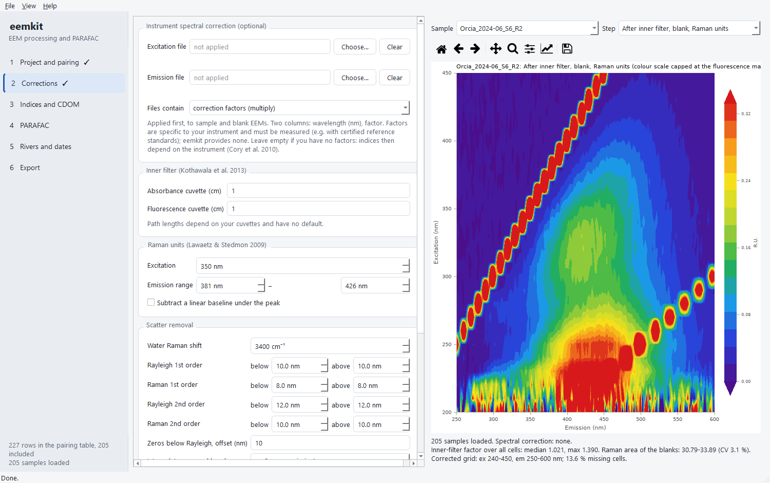
|
|
57
|
+
|
|
58
|
+
## What it does
|
|
59
|
+
|
|
60
|
+
* **Import** Agilent Cary Eclipse 3-D EEMs and Cary 60 absorbance spectra
|
|
61
|
+
(CSV "ASCII with log"), with the instrument settings from the file log.
|
|
62
|
+
Samples, blanks and absorbance spectra are paired through an explicit,
|
|
63
|
+
hand-editable table: nothing is matched silently.
|
|
64
|
+
* **Correct** in a fixed, enforced order: instrument spectral correction
|
|
65
|
+
(optional), absorbance blank, inner-filter effect (Kothawala et al. 2013),
|
|
66
|
+
blank subtraction, Raman units (Lawaetz & Stedmon 2009), Rayleigh and Raman
|
|
67
|
+
scatter removal, crop. Values that depend on the measurement, such as cuvette
|
|
68
|
+
path lengths, have no defaults.
|
|
69
|
+
* **Indices**: fluorescence index, humification and biological indices, Coble
|
|
70
|
+
peaks.
|
|
71
|
+
* **CDOM metrics** from the absorbance spectra: a254, a350, spectral slopes
|
|
72
|
+
S275–295 and S350–400, slope ratio (Helms et al. 2008), E2:E3 and SUVA254,
|
|
73
|
+
after a baseline correction; values the signal cannot support are left
|
|
74
|
+
empty with the reason.
|
|
75
|
+
* **PARAFAC** with non-negativity and missing values, random starts, core
|
|
76
|
+
consistency, leverage and residuals, split-half validation (Murphy et al.
|
|
77
|
+
2013) and export to OpenFluor.
|
|
78
|
+
* **Rivers, sites and dates**: any index, CDOM metric or PARAFAC component
|
|
79
|
+
compared between sampling campaigns within each river (replicates averaged
|
|
80
|
+
per site, Kruskal–Wallis and Dunn tests), along the river and against
|
|
81
|
+
covariates such as discharge or rainfall, with a warning when rivers and
|
|
82
|
+
dates cannot be separated.
|
|
83
|
+
* **Figures** for publication, and a **desktop application** (PySide6, light
|
|
84
|
+
and dark themes) that drives the whole chain without code.
|
|
85
|
+
* **Provenance**: data are `xarray` datasets that carry their metadata and the
|
|
86
|
+
full processing history; one settings file drives both scripts and the
|
|
87
|
+
application.
|
|
88
|
+
|
|
89
|
+
## Install
|
|
90
|
+
|
|
91
|
+
You need Python 3.11 or later (on Windows, tick *Add python.exe to PATH* when
|
|
92
|
+
installing it). The `[gui]` part adds the desktop application and the
|
|
93
|
+
figures:
|
|
94
|
+
|
|
95
|
+
```bash
|
|
96
|
+
python -m pip install "eemkit[gui]"
|
|
97
|
+
```
|
|
98
|
+
|
|
99
|
+
Then start the application with:
|
|
100
|
+
|
|
101
|
+
```bash
|
|
102
|
+
python -m eemkit.gui
|
|
103
|
+
```
|
|
104
|
+
|
|
105
|
+
For the library alone, leave out `[gui]` (or use `[plot]` for figures
|
|
106
|
+
without the application). A stand-alone Windows build of the application,
|
|
107
|
+
which needs no Python, is attached to each
|
|
108
|
+
[release](https://github.com/LowCostSensor/eemkit/releases).
|
|
109
|
+
|
|
110
|
+
To update to the latest release:
|
|
111
|
+
|
|
112
|
+
```bash
|
|
113
|
+
python -m pip install --upgrade "eemkit[gui]"
|
|
114
|
+
```
|
|
115
|
+
|
|
116
|
+
The development version, with changes not yet released, installs from GitHub:
|
|
117
|
+
|
|
118
|
+
```bash
|
|
119
|
+
python -m pip install --force-reinstall "eemkit[gui] @ https://github.com/LowCostSensor/eemkit/archive/refs/heads/main.zip"
|
|
120
|
+
```
|
|
121
|
+
|
|
122
|
+
`python -m pip show eemkit` tells which version is installed; the changes of
|
|
123
|
+
each version are in the
|
|
124
|
+
[changelog](https://github.com/LowCostSensor/eemkit/blob/main/CHANGELOG.md).
|
|
125
|
+
|
|
126
|
+
## Quick start
|
|
127
|
+
|
|
128
|
+
```python
|
|
129
|
+
from eemkit import pipeline
|
|
130
|
+
|
|
131
|
+
s = pipeline.load_settings("project.toml") # data folder, pairing table, parameters
|
|
132
|
+
raw = pipeline.load(s, base=".")
|
|
133
|
+
after_raman = pipeline.correct_until_raman(raw, s, base=".")
|
|
134
|
+
corrected = pipeline.finish_corrections(after_raman, s)
|
|
135
|
+
indices = pipeline.compute_indices(after_raman, s)
|
|
136
|
+
|
|
137
|
+
ds = pipeline.parafac_input(corrected, s)
|
|
138
|
+
exploration = pipeline.explore(ds, s) # 2..7 components, split-half validation
|
|
139
|
+
model, split = pipeline.fit_final(ds, s) # the number of components you chose
|
|
140
|
+
pipeline.export_results("results", s, corrected=corrected, indices=indices,
|
|
141
|
+
exploration=exploration, model=model, split=split)
|
|
142
|
+
```
|
|
143
|
+
|
|
144
|
+
Or start the application (`python -m eemkit.gui`) and open the same
|
|
145
|
+
`project.toml`.
|
|
146
|
+
|
|
147
|
+
Every function can also be used on its own; see the
|
|
148
|
+
[documentation](https://lowcostsensor.github.io/eemkit/).
|
|
149
|
+
|
|
150
|
+
## Validation
|
|
151
|
+
|
|
152
|
+
On 205 river-water samples (Ombrone basin, Italy; Polvani et al. 2026) eemkit
|
|
153
|
+
was compared with the R package staRdom 1.1.32 (Pucher et al. 2019):
|
|
154
|
+
|
|
155
|
+
* corrected EEMs agree to a median relative difference of 2.2 × 10⁻⁴ (the
|
|
156
|
+
remainder is the numerical integration of the Raman area);
|
|
157
|
+
* FI, BIX and Coble peaks agree to machine precision, HIX to 3 × 10⁻⁴;
|
|
158
|
+
* the 3-component PARAFAC models have Tucker congruence ≥ 0.999 for every
|
|
159
|
+
excitation and emission loading.
|
|
160
|
+
|
|
161
|
+
The scripts and the full report are in
|
|
162
|
+
[ombrone-fdom](https://github.com/LowCostSensor/ombrone-fdom).
|
|
163
|
+
|
|
164
|
+
## Development
|
|
165
|
+
|
|
166
|
+
```bash
|
|
167
|
+
git clone https://github.com/LowCostSensor/eemkit
|
|
168
|
+
cd eemkit
|
|
169
|
+
pip install -e ".[dev]"
|
|
170
|
+
pytest
|
|
171
|
+
```
|
|
172
|
+
|
|
173
|
+
Tests that need the real dataset are skipped unless `EEMKIT_TEST_DATA` points
|
|
174
|
+
to its root folder. Contributions and bug reports are welcome: see
|
|
175
|
+
[CONTRIBUTING.md](https://github.com/LowCostSensor/eemkit/blob/main/CONTRIBUTING.md).
|
|
176
|
+
|
|
177
|
+
## Citation
|
|
178
|
+
|
|
179
|
+
If you use eemkit, please cite it (see
|
|
180
|
+
[CITATION.cff](https://github.com/LowCostSensor/eemkit/blob/main/CITATION.cff); a DOI is
|
|
181
|
+
issued on Zenodo for every release) and the methods it implements, listed in
|
|
182
|
+
the documentation of each step.
|
|
183
|
+
|
|
184
|
+
## License
|
|
185
|
+
|
|
186
|
+
GNU General Public License v3.0 or later. See
|
|
187
|
+
[LICENSE](https://github.com/LowCostSensor/eemkit/blob/main/LICENSE).
|
|
188
|
+
|
|
189
|
+
## References
|
|
190
|
+
|
|
191
|
+
Kothawala et al. (2013) *Limnol. Oceanogr. Methods* 11, 616–630 ·
|
|
192
|
+
Lawaetz & Stedmon (2009) *Appl. Spectrosc.* 63, 936–940 ·
|
|
193
|
+
Murphy et al. (2013) *Anal. Methods* 5, 6557–6566 ·
|
|
194
|
+
Polvani et al. (2026) *Environ. Pollut.* 396, 127858 ·
|
|
195
|
+
Pucher et al. (2019) *Water* 11, 2366.
|