divinity-forecast 0.2.0__py3-none-any.whl
This diff represents the content of publicly available package versions that have been released to one of the supported registries. The information contained in this diff is provided for informational purposes only and reflects changes between package versions as they appear in their respective public registries.
- divinity/__init__.py +32 -0
- divinity/features.py +93 -0
- divinity/forecaster.py +466 -0
- divinity/legacy.py +138 -0
- divinity/periods.py +106 -0
- divinity/plotting.py +77 -0
- divinity/residuals.py +146 -0
- divinity/selection.py +157 -0
- divinity/synthetic.py +217 -0
- divinity_forecast-0.2.0.dist-info/METADATA +251 -0
- divinity_forecast-0.2.0.dist-info/RECORD +14 -0
- divinity_forecast-0.2.0.dist-info/WHEEL +5 -0
- divinity_forecast-0.2.0.dist-info/licenses/LICENSE +201 -0
- divinity_forecast-0.2.0.dist-info/top_level.txt +1 -0
divinity/synthetic.py
ADDED
|
@@ -0,0 +1,217 @@
|
|
|
1
|
+
"""
|
|
2
|
+
Synthetic test series with known structure, split into history and future.
|
|
3
|
+
|
|
4
|
+
These are used by the tests, the README figures and the demo notebook, and
|
|
5
|
+
are handy for experimenting. Every scenario is reproducible from its seed.
|
|
6
|
+
"""
|
|
7
|
+
|
|
8
|
+
from dataclasses import dataclass, field
|
|
9
|
+
|
|
10
|
+
import numpy as np
|
|
11
|
+
import pandas as pd
|
|
12
|
+
|
|
13
|
+
|
|
14
|
+
@dataclass
|
|
15
|
+
class Scenario:
|
|
16
|
+
"""
|
|
17
|
+
A synthetic forecasting problem.
|
|
18
|
+
|
|
19
|
+
:param name: short identifier.
|
|
20
|
+
:param description: what the series contains and what a good model
|
|
21
|
+
should do with it.
|
|
22
|
+
:param history: training series.
|
|
23
|
+
:param future: true values over the forecast horizon.
|
|
24
|
+
:param options: Forecaster arguments this scenario calls for.
|
|
25
|
+
"""
|
|
26
|
+
|
|
27
|
+
name: str
|
|
28
|
+
description: str
|
|
29
|
+
history: pd.Series
|
|
30
|
+
future: pd.Series
|
|
31
|
+
options: dict = field(default_factory=dict)
|
|
32
|
+
|
|
33
|
+
@property
|
|
34
|
+
def steps(self):
|
|
35
|
+
return len(self.future)
|
|
36
|
+
|
|
37
|
+
|
|
38
|
+
def _split(y, horizon):
|
|
39
|
+
return y.iloc[:-horizon], y.iloc[-horizon:]
|
|
40
|
+
|
|
41
|
+
|
|
42
|
+
def trend_seasonal(seed=0, n=200, horizon=40):
|
|
43
|
+
rng = np.random.default_rng(seed)
|
|
44
|
+
t = np.arange(n + horizon)
|
|
45
|
+
y = 0.05 * t + 2 * np.sin(2 * np.pi * t / 20) + rng.normal(0, 0.5, len(t))
|
|
46
|
+
history, future = _split(pd.Series(y), horizon)
|
|
47
|
+
return Scenario(
|
|
48
|
+
"trend_seasonal",
|
|
49
|
+
"Linear trend plus a period 20 cycle and noise. The standard case.",
|
|
50
|
+
history,
|
|
51
|
+
future,
|
|
52
|
+
)
|
|
53
|
+
|
|
54
|
+
|
|
55
|
+
def daily_multi_seasonal(seed=0, years=3, horizon=90):
|
|
56
|
+
rng = np.random.default_rng(seed)
|
|
57
|
+
dates = pd.date_range("2022-01-01", periods=int(365.25 * years) + horizon, freq="D")
|
|
58
|
+
t = np.arange(len(dates))
|
|
59
|
+
weekly = np.where(dates.day_of_week >= 5, -3.0, 0.6) # sharp weekend dip
|
|
60
|
+
yearly = 4 * np.sin(2 * np.pi * t / 365.25)
|
|
61
|
+
y = 50 + 0.01 * t + weekly + yearly + rng.normal(0, 1.0, len(t))
|
|
62
|
+
history, future = _split(pd.Series(y, index=dates), horizon)
|
|
63
|
+
return Scenario(
|
|
64
|
+
"daily_multi_seasonal",
|
|
65
|
+
"Daily data with a square weekend dip and a yearly cycle. Weekly and "
|
|
66
|
+
"yearly periods come from the date frequency.",
|
|
67
|
+
history,
|
|
68
|
+
future,
|
|
69
|
+
)
|
|
70
|
+
|
|
71
|
+
|
|
72
|
+
def monthly_multiplicative(seed=0, years=12, horizon=24):
|
|
73
|
+
rng = np.random.default_rng(seed)
|
|
74
|
+
dates = pd.date_range("2012-01-01", periods=12 * years + horizon, freq="MS")
|
|
75
|
+
t = np.arange(len(dates))
|
|
76
|
+
log_y = (
|
|
77
|
+
np.log(100)
|
|
78
|
+
+ 0.01 * t
|
|
79
|
+
+ 0.2 * np.sin(2 * np.pi * t / 12)
|
|
80
|
+
+ 0.1 * np.cos(4 * np.pi * t / 12)
|
|
81
|
+
+ rng.normal(0, 0.04, len(t))
|
|
82
|
+
)
|
|
83
|
+
history, future = _split(pd.Series(np.exp(log_y), index=dates), horizon)
|
|
84
|
+
return Scenario(
|
|
85
|
+
"monthly_multiplicative",
|
|
86
|
+
"Monthly growth series whose seasonal swing grows with its level. "
|
|
87
|
+
"Fitted on the log scale.",
|
|
88
|
+
history,
|
|
89
|
+
future,
|
|
90
|
+
{"log": True},
|
|
91
|
+
)
|
|
92
|
+
|
|
93
|
+
|
|
94
|
+
def white_noise(seed=0, n=200, horizon=50):
|
|
95
|
+
rng = np.random.default_rng(seed)
|
|
96
|
+
history, future = _split(pd.Series(10 + rng.normal(0, 1, n + horizon)), horizon)
|
|
97
|
+
return Scenario(
|
|
98
|
+
"white_noise",
|
|
99
|
+
"Pure noise around a constant. There is nothing to find, so the "
|
|
100
|
+
"forecast should be flat with no invented seasonality or trend.",
|
|
101
|
+
history,
|
|
102
|
+
future,
|
|
103
|
+
)
|
|
104
|
+
|
|
105
|
+
|
|
106
|
+
def random_walk(seed=0, n=300, horizon=60):
|
|
107
|
+
rng = np.random.default_rng(seed)
|
|
108
|
+
y = np.cumsum(rng.normal(0, 1, n + horizon))
|
|
109
|
+
history, future = _split(pd.Series(y), horizon)
|
|
110
|
+
return Scenario(
|
|
111
|
+
"random_walk",
|
|
112
|
+
"A random walk. It wanders and looks trendy by chance, so the model "
|
|
113
|
+
"should not extrapolate a confident trend and its interval should "
|
|
114
|
+
"widen with the horizon.",
|
|
115
|
+
history,
|
|
116
|
+
future,
|
|
117
|
+
)
|
|
118
|
+
|
|
119
|
+
|
|
120
|
+
def ar1(seed=0, n=200, horizon=50, phi=0.85):
|
|
121
|
+
rng = np.random.default_rng(seed)
|
|
122
|
+
e = rng.normal(0, 1, n + horizon + 100)
|
|
123
|
+
u = np.zeros_like(e)
|
|
124
|
+
for i in range(1, len(e)):
|
|
125
|
+
u[i] = phi * u[i - 1] + e[i]
|
|
126
|
+
history, future = _split(pd.Series(20 + u[100:]), horizon)
|
|
127
|
+
return Scenario(
|
|
128
|
+
"ar1",
|
|
129
|
+
"Strongly autocorrelated but stationary. Forecast should decay back "
|
|
130
|
+
"towards the mean rather than run off as if it were a random walk.",
|
|
131
|
+
history,
|
|
132
|
+
future,
|
|
133
|
+
)
|
|
134
|
+
|
|
135
|
+
|
|
136
|
+
def missing_data(seed=0, n=200, horizon=40):
|
|
137
|
+
base = trend_seasonal(seed, n, horizon)
|
|
138
|
+
rng = np.random.default_rng(seed + 1000)
|
|
139
|
+
history = base.history.copy()
|
|
140
|
+
history[rng.random(n) < 0.15] = np.nan
|
|
141
|
+
history.iloc[90:115] = np.nan
|
|
142
|
+
return Scenario(
|
|
143
|
+
"missing_data",
|
|
144
|
+
"The standard case with 15% of points missing at random and a " "25 step gap.",
|
|
145
|
+
history,
|
|
146
|
+
base.future,
|
|
147
|
+
)
|
|
148
|
+
|
|
149
|
+
|
|
150
|
+
def unknown_period(seed=0, n=240, horizon=60):
|
|
151
|
+
rng = np.random.default_rng(seed)
|
|
152
|
+
t = np.arange(n + horizon)
|
|
153
|
+
y = 3 * np.sin(2 * np.pi * t / 17.3) + rng.normal(0, 1, len(t))
|
|
154
|
+
history, future = _split(pd.Series(y), horizon)
|
|
155
|
+
return Scenario(
|
|
156
|
+
"unknown_period",
|
|
157
|
+
"A period of 17.3 steps that nobody told the model about. It has to "
|
|
158
|
+
"find it in the periodogram.",
|
|
159
|
+
history,
|
|
160
|
+
future,
|
|
161
|
+
)
|
|
162
|
+
|
|
163
|
+
|
|
164
|
+
def outliers(seed=0, n=200, horizon=40):
|
|
165
|
+
base = trend_seasonal(seed, n, horizon)
|
|
166
|
+
history = base.history.copy()
|
|
167
|
+
history.iloc[[40, 120, 170]] += np.array([15.0, -12.0, 18.0])
|
|
168
|
+
return Scenario(
|
|
169
|
+
"outliers",
|
|
170
|
+
"The standard case with three large one-off spikes.",
|
|
171
|
+
history,
|
|
172
|
+
base.future,
|
|
173
|
+
)
|
|
174
|
+
|
|
175
|
+
|
|
176
|
+
def short_daily(seed=0, days=35, horizon=14):
|
|
177
|
+
rng = np.random.default_rng(seed)
|
|
178
|
+
dates = pd.date_range("2024-03-01", periods=days + horizon, freq="D")
|
|
179
|
+
weekly = np.where(dates.day_of_week >= 5, 5.0, 0.0)
|
|
180
|
+
y = 20 + weekly + rng.normal(0, 1, len(dates))
|
|
181
|
+
history, future = _split(pd.Series(y, index=dates), horizon)
|
|
182
|
+
return Scenario(
|
|
183
|
+
"short_daily",
|
|
184
|
+
"Only five weeks of daily data. The yearly default period cannot be "
|
|
185
|
+
"estimated and must be ignored, while the weekly cycle is still used.",
|
|
186
|
+
history,
|
|
187
|
+
future,
|
|
188
|
+
)
|
|
189
|
+
|
|
190
|
+
|
|
191
|
+
SCENARIOS = {
|
|
192
|
+
f.__name__: f
|
|
193
|
+
for f in (
|
|
194
|
+
trend_seasonal,
|
|
195
|
+
daily_multi_seasonal,
|
|
196
|
+
monthly_multiplicative,
|
|
197
|
+
white_noise,
|
|
198
|
+
random_walk,
|
|
199
|
+
ar1,
|
|
200
|
+
missing_data,
|
|
201
|
+
unknown_period,
|
|
202
|
+
outliers,
|
|
203
|
+
short_daily,
|
|
204
|
+
)
|
|
205
|
+
}
|
|
206
|
+
|
|
207
|
+
|
|
208
|
+
def make(name, seed=0, **kwargs):
|
|
209
|
+
"""
|
|
210
|
+
Build a scenario by name, e.g. ``make("random_walk", seed=3)``.
|
|
211
|
+
"""
|
|
212
|
+
try:
|
|
213
|
+
return SCENARIOS[name](seed=seed, **kwargs)
|
|
214
|
+
except KeyError:
|
|
215
|
+
raise ValueError(
|
|
216
|
+
"unknown scenario {!r}, choose from {}".format(name, sorted(SCENARIOS))
|
|
217
|
+
) from None
|
|
@@ -0,0 +1,251 @@
|
|
|
1
|
+
Metadata-Version: 2.4
|
|
2
|
+
Name: divinity-forecast
|
|
3
|
+
Version: 0.2.0
|
|
4
|
+
Summary: Automatic timeseries forecasting with honest prediction intervals
|
|
5
|
+
Author-email: dstarkey23 <drds.gh1@gmail.com>
|
|
6
|
+
License-Expression: Apache-2.0
|
|
7
|
+
Project-URL: Homepage, https://github.com/drds1/divinity
|
|
8
|
+
Requires-Python: >=3.10
|
|
9
|
+
Description-Content-Type: text/markdown
|
|
10
|
+
License-File: LICENSE
|
|
11
|
+
Requires-Dist: numpy>=1.24
|
|
12
|
+
Requires-Dist: pandas>=2.0
|
|
13
|
+
Requires-Dist: scipy>=1.10
|
|
14
|
+
Requires-Dist: statsmodels>=0.14
|
|
15
|
+
Requires-Dist: matplotlib>=3.7
|
|
16
|
+
Provides-Extra: dev
|
|
17
|
+
Requires-Dist: pytest>=8; extra == "dev"
|
|
18
|
+
Requires-Dist: pre-commit>=3; extra == "dev"
|
|
19
|
+
Requires-Dist: nbclient>=0.10; extra == "dev"
|
|
20
|
+
Requires-Dist: nbformat>=5.10; extra == "dev"
|
|
21
|
+
Requires-Dist: ipykernel>=6; extra == "dev"
|
|
22
|
+
Dynamic: license-file
|
|
23
|
+
|
|
24
|
+
# Divinity
|
|
25
|
+
|
|
26
|
+
[](https://github.com/psf/black)
|
|
27
|
+
|
|
28
|
+
Automatic timeseries forecasting with prediction intervals you can trust.
|
|
29
|
+
|
|
30
|
+
Give it a series and a horizon. Divinity decides whether there is a trend, which seasonal cycles are real and how much autocorrelation is left over. It returns a forecast with an interval that widens as much as the data say it should, and no more.
|
|
31
|
+
|
|
32
|
+
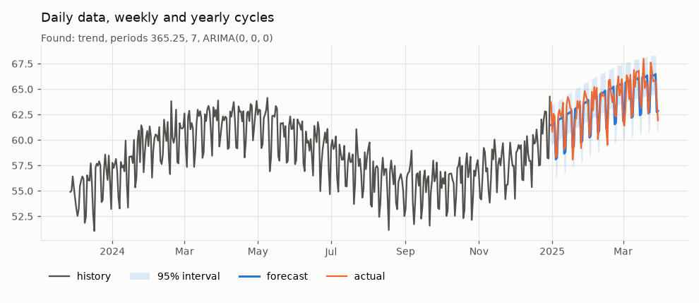
|
|
33
|
+
|
|
34
|
+
## Install
|
|
35
|
+
|
|
36
|
+
```bash
|
|
37
|
+
pip install divinity-forecast
|
|
38
|
+
```
|
|
39
|
+
|
|
40
|
+
The package installs as `divinity-forecast` but is imported as `divinity`. Version 0.1 was published as `divinity` and is no longer maintained there.
|
|
41
|
+
|
|
42
|
+
Or from a clone, with the development tools
|
|
43
|
+
|
|
44
|
+
```bash
|
|
45
|
+
pip install -e ".[dev]"
|
|
46
|
+
```
|
|
47
|
+
|
|
48
|
+
Python 3.10 or later.
|
|
49
|
+
|
|
50
|
+
## Quick start
|
|
51
|
+
|
|
52
|
+
```python
|
|
53
|
+
import divinity as dv
|
|
54
|
+
|
|
55
|
+
model = dv.Forecaster().fit(y) # y is a pandas Series, numpy array or list
|
|
56
|
+
result = model.predict(steps=30) # DataFrame with forecast, lower, upper
|
|
57
|
+
print(model.summary())
|
|
58
|
+
model.plot(result)
|
|
59
|
+
```
|
|
60
|
+
|
|
61
|
+
```text
|
|
62
|
+
Divinity forecaster
|
|
63
|
+
observations 1095
|
|
64
|
+
frequency D
|
|
65
|
+
log scale no
|
|
66
|
+
trend linear
|
|
67
|
+
seasonality 365.25 (1 harmonic), 7 (3 harmonics)
|
|
68
|
+
residuals ARIMA(0, 0, 0)
|
|
69
|
+
```
|
|
70
|
+
|
|
71
|
+
Or in one line
|
|
72
|
+
|
|
73
|
+
```python
|
|
74
|
+
result = dv.forecast(y, steps=30)
|
|
75
|
+
```
|
|
76
|
+
|
|
77
|
+
`result` is indexed by future time. A Series with a `DatetimeIndex` gives future dates, anything else gives integer steps following on from the data.
|
|
78
|
+
|
|
79
|
+
```text
|
|
80
|
+
forecast lower upper
|
|
81
|
+
2024-12-31 61.48 59.55 63.41
|
|
82
|
+
2025-01-01 61.55 59.62 63.49
|
|
83
|
+
...
|
|
84
|
+
```
|
|
85
|
+
|
|
86
|
+
The [demo notebook](https://github.com/drds1/divinity/blob/master/notebooks/demo.ipynb) walks through everything below with live examples.
|
|
87
|
+
|
|
88
|
+
## How it works
|
|
89
|
+
|
|
90
|
+
The series is modelled as a constant, plus an optional linear trend, plus Fourier terms for each seasonal period, plus ARIMA errors (regression with ARIMA errors).
|
|
91
|
+
|
|
92
|
+
1. **Candidate periods.** These come from the date frequency (7 and 365.25 for daily data, 12 for monthly, 24 and 168 for hourly and so on) and from peaks in the periodogram, so a cycle nobody mentioned can still be found. A period is only considered if the data cover at least two full cycles.
|
|
93
|
+
2. **Feature selection.** Trend and seasonal terms are added one at a time while they improve BIC. Extra harmonics of a period (for sharper, non-sinusoidal shapes) are only tried once the lower harmonic is in. There is an additional penalty for searching over many candidates. Without it, testing dozens of periods on noise will find one by chance.
|
|
94
|
+
3. **Random walk or not?** Before choosing any features, an augmented Dickey-Fuller test is run on what is left after removing the trend and the known periods. Detected periods are left out because they might be spurious. Testing first matters. On a random walk, spurious features soak up the wander and make the leftovers look stationary, so a test afterwards confirms its own mistake.
|
|
95
|
+
4. **Allowing for autocorrelation.** Least squares assumes independent errors, and on a random walk it declares almost any trend "significant". If the series has a unit root, features are selected on differenced data. Otherwise the autocorrelation of the residuals is estimated and features are reselected on quasi-differenced data (feasible GLS), repeating until the choice settles. The ARIMA order for what remains is chosen by BIC over a small grid.
|
|
96
|
+
5. **Joint fit and intervals.** Features and ARIMA errors are fitted together by maximum likelihood. Forecast intervals combine the ARIMA forecast variance with the uncertainty in the trend and seasonal coefficients, which matters most when extrapolating a trend a long way. Student t quantiles allow for the noise level being estimated, which matters for short series.
|
|
97
|
+
|
|
98
|
+
The fitted model does not depend on the forecast horizon, so `predict(10)` is exactly the first ten rows of `predict(100)`.
|
|
99
|
+
|
|
100
|
+
## Can it be fooled?
|
|
101
|
+
|
|
102
|
+
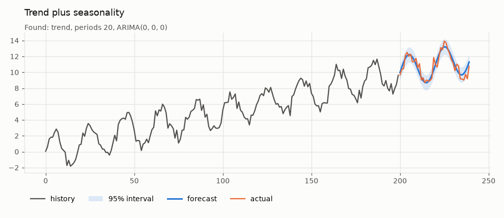
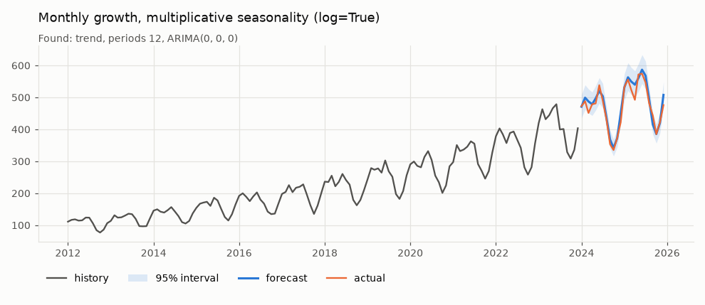
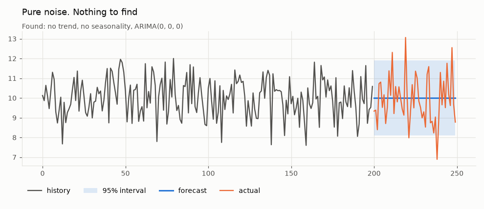
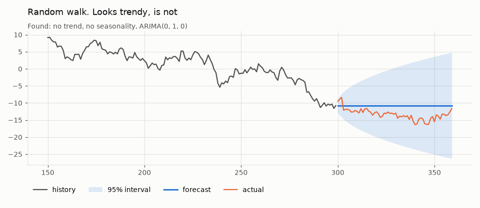
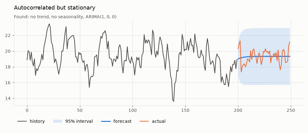
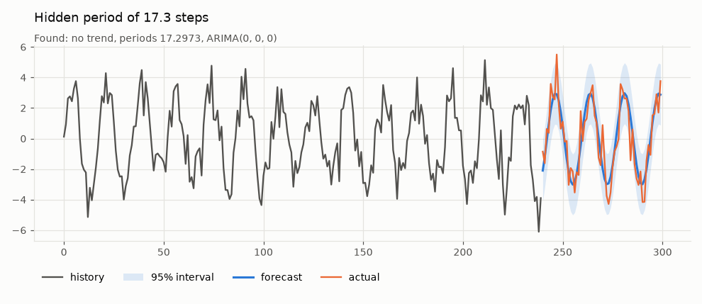
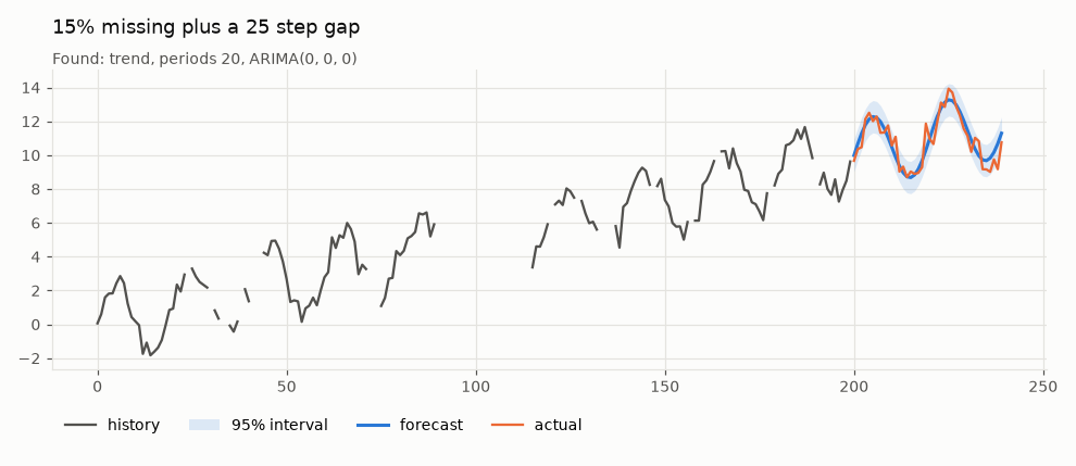
The cases below are built to catch out a naive forecaster. Each was generated by [`divinity.synthetic`](https://github.com/drds1/divinity/blob/master/divinity/synthetic.py) with seed 0, the same seed the smoke tests use, so none of them were picked because they looked good. In every chart the orange line is the true future, which the model never saw.
|
|
103
|
+
|
|
104
|
+
### The standard case
|
|
105
|
+
|
|
106
|
+
A linear trend, a 20 step cycle and noise. Neither component is specified.
|
|
107
|
+
|
|
108
|
+
|
|
109
|
+
|
|
110
|
+
### Multiplicative seasonality
|
|
111
|
+
|
|
112
|
+
The seasonal swing grows with the level. Fitting with `log=True` handles this.
|
|
113
|
+
|
|
114
|
+
|
|
115
|
+
|
|
116
|
+
### Pure noise
|
|
117
|
+
|
|
118
|
+
There is nothing to find. A model that looks hard enough for structure will find some anyway. Divinity returns a flat forecast at the mean.
|
|
119
|
+
|
|
120
|
+
|
|
121
|
+
|
|
122
|
+
### A random walk
|
|
123
|
+
|
|
124
|
+
Random walks look trendy. Ordinary least squares picks a "significant" trend in the large majority of them, which is then extrapolated with false confidence. Divinity finds no trend or seasonality, switches to a differenced model and lets the interval fan out.
|
|
125
|
+
|
|
126
|
+
|
|
127
|
+
|
|
128
|
+
### Autocorrelated but stationary
|
|
129
|
+
|
|
130
|
+
The opposite trap. The series wanders but always returns to its mean. The forecast decays back towards the mean rather than treating it as a random walk.
|
|
131
|
+
|
|
132
|
+
|
|
133
|
+
|
|
134
|
+
### A period nobody mentioned
|
|
135
|
+
|
|
136
|
+
A cycle of 17.3 steps on integer data with no frequency. It is found from the periodogram, including the fractional part.
|
|
137
|
+
|
|
138
|
+
|
|
139
|
+
|
|
140
|
+
### Missing data
|
|
141
|
+
|
|
142
|
+
15% of values missing at random plus a 25 step gap. Gaps are handled natively, with no interpolation needed.
|
|
143
|
+
|
|
144
|
+
|
|
145
|
+
|
|
146
|
+
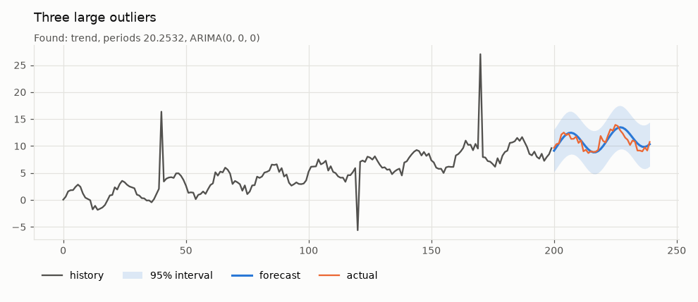
### Outliers
|
|
147
|
+
|
|
148
|
+
Three large one-off spikes.
|
|
149
|
+
|
|
150
|
+
|
|
151
|
+
|
|
152
|
+
### Very short history
|
|
153
|
+
|
|
154
|
+
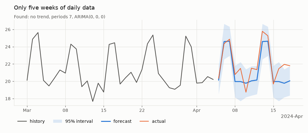
Five weeks of daily data. The yearly default period cannot be estimated from that and is dropped automatically, while the weekly cycle is kept.
|
|
155
|
+
|
|
156
|
+
|
|
157
|
+
|
|
158
|
+
### Across 100 random seeds per case
|
|
159
|
+
|
|
160
|
+
One chart per case could still be luck, so [`benchmarks/coverage.py`](https://github.com/drds1/divinity/blob/master/benchmarks/coverage.py) refits every scenario on 100 different seeds. *Interval coverage* is how often the true future falls inside the 95% interval, so it should be close to 95%. *Structure found* is how often the model chose the components the series was built with (for example no seasonality on noise, differencing on a random walk, period 17.3 when it is hidden). *RMSE vs naive* compares the error with simply repeating the last observed value, where below 1 is better.
|
|
161
|
+
|
|
162
|
+
| scenario | runs | 95% interval coverage | structure found | RMSE vs naive |
|
|
163
|
+
|---|---:|---:|---:|---:|
|
|
164
|
+
| `trend_seasonal` | 100 | 94.3% | 100% | 0.24 |
|
|
165
|
+
| `daily_multi_seasonal` | 100 | 95.1% | 100% | 0.32 |
|
|
166
|
+
| `monthly_multiplicative` | 100 | 93.9% | 97% | 0.20 |
|
|
167
|
+
| `white_noise` | 100 | 94.8% | 98% | 0.75 |
|
|
168
|
+
| `random_walk` | 100 | 93.9% | 94% | 1.04 |
|
|
169
|
+
| `ar1` | 100 | 91.8% | 88% | 0.82 |
|
|
170
|
+
| `missing_data` | 100 | 93.9% | 100% | 0.23 |
|
|
171
|
+
| `unknown_period` | 100 | 95.0% | 100% | 0.27 |
|
|
172
|
+
| `outliers` | 100 | 100.0% | 100% | 0.43 |
|
|
173
|
+
| `short_daily` | 100 | 91.4% | 100% | 0.38 |
|
|
174
|
+
|
|
175
|
+
How to read the weaker rows
|
|
176
|
+
|
|
177
|
+
- **`ar1` (91.8%).** Autoregressive coefficients estimated from 200 points are biased slightly towards zero, so the intervals come out a little narrow. In 12% of runs the model reads the series as a random walk or adds a small trend. Both are hard to tell apart from a strongly autocorrelated series of this length.
|
|
178
|
+
- **`random_walk` (RMSE 1.04).** For a random walk the naive forecast is the best possible point forecast, so about 1.0 is the floor. What matters here is the interval, and 94% coverage means the fan is honest.
|
|
179
|
+
- **`short_daily` (91.4%).** 35 points carrying seven seasonal coefficients leaves little to estimate the noise from, even with t quantiles.
|
|
180
|
+
- **`outliers` (100%).** The spikes inflate the estimated noise, so the intervals are wider than they need to be. This errs in the safe direction.
|
|
181
|
+
|
|
182
|
+
Regenerate it with
|
|
183
|
+
|
|
184
|
+
```bash
|
|
185
|
+
python benchmarks/coverage.py --seeds 100
|
|
186
|
+
```
|
|
187
|
+
|
|
188
|
+
## Options
|
|
189
|
+
|
|
190
|
+
```python
|
|
191
|
+
dv.Forecaster(
|
|
192
|
+
seasonal_periods="auto", # "auto" (from the frequency), a list of periods, or None
|
|
193
|
+
detect_periods=True, # also look for periods in the data
|
|
194
|
+
max_detected_periods=3,
|
|
195
|
+
max_harmonics=3, # Fourier harmonics per period, more allow sharper shapes
|
|
196
|
+
trend="auto", # "auto", "linear" or None
|
|
197
|
+
arima="auto", # "auto", a (p, d, q) tuple, or None for white noise
|
|
198
|
+
log=False, # fit on the log scale, for growth with growing seasonality
|
|
199
|
+
interval=0.95, # default interval coverage
|
|
200
|
+
search_penalty=1.0, # higher is more reluctant to add seasonality, 0 is plain BIC
|
|
201
|
+
)
|
|
202
|
+
```
|
|
203
|
+
|
|
204
|
+
Useful things on a fitted model
|
|
205
|
+
|
|
206
|
+
| | |
|
|
207
|
+
|---|---|
|
|
208
|
+
| `predict(steps, interval=None)` | forecast DataFrame (`forecast`, `lower`, `upper`) |
|
|
209
|
+
| `plot(forecast, actual=None, history=None)` | chart, returns the matplotlib Axes |
|
|
210
|
+
| `summary()` | readable description of what was chosen |
|
|
211
|
+
| `components_` | the same as a dict |
|
|
212
|
+
| `fitted_` | in-sample one step ahead predictions |
|
|
213
|
+
|
|
214
|
+
If dates are missing entirely from a `DatetimeIndex` the frequency cannot be inferred. Pass it, for example `fit(y, freq="D")`, and the gaps become missing values.
|
|
215
|
+
|
|
216
|
+
## Limitations
|
|
217
|
+
|
|
218
|
+
- Trends are linear. A curve or saturation will be extrapolated as a straight line.
|
|
219
|
+
- Level shifts and regime changes are not modelled.
|
|
220
|
+
- Outliers are not removed. They widen the interval a little instead.
|
|
221
|
+
- Seasonal shape is fixed (or proportional to the level with `log=True`).
|
|
222
|
+
- One series at a time, with no external regressors.
|
|
223
|
+
|
|
224
|
+
## Development
|
|
225
|
+
|
|
226
|
+
```bash
|
|
227
|
+
pip install -e ".[dev]"
|
|
228
|
+
pre-commit install
|
|
229
|
+
pytest -m "not slow" # fast unit and smoke tests
|
|
230
|
+
pytest # also the coverage checks over many seeds (a few minutes)
|
|
231
|
+
python docs/make_figures.py
|
|
232
|
+
```
|
|
233
|
+
|
|
234
|
+
The code is in [`divinity/`](https://github.com/drds1/divinity/tree/master/divinity/), with one module per stage: `periods.py` (candidate periods), `features.py` (trend and Fourier terms), `selection.py` (feature selection), `residuals.py` (ARIMA order) and `forecaster.py` (the `Forecaster` class tying them together). `synthetic.py` holds the test scenarios.
|
|
235
|
+
|
|
236
|
+
### Upgrading from 0.1
|
|
237
|
+
|
|
238
|
+
The old `divinity.divinity(forecast_length=...)` class still works but is deprecated and now runs the new model underneath. Replace
|
|
239
|
+
|
|
240
|
+
```python
|
|
241
|
+
model = dv.divinity(forecast_length=20)
|
|
242
|
+
model.fit(y)
|
|
243
|
+
y_pred = model.predict()
|
|
244
|
+
```
|
|
245
|
+
|
|
246
|
+
with
|
|
247
|
+
|
|
248
|
+
```python
|
|
249
|
+
result = dv.Forecaster().fit(y).predict(20)
|
|
250
|
+
y_pred = result["forecast"]
|
|
251
|
+
```
|
|
@@ -0,0 +1,14 @@
|
|
|
1
|
+
divinity/__init__.py,sha256=IY4Z0aZa_uYUvWy0uxhjgXNLNXlb1P6HKBbcsX3majo,556
|
|
2
|
+
divinity/features.py,sha256=b2B6u9WbLmucjA-30f59QV7N1t1icKOCMtN7PRIbiJE,3063
|
|
3
|
+
divinity/forecaster.py,sha256=C9qFqpBlsXCugOyNctdb2cKtT0ohGesY_AHVlBCtEmo,18108
|
|
4
|
+
divinity/legacy.py,sha256=OYZvniAnJqi38FxBvjdg3jJS3qOLkjAaU-Ksh7xyQfw,4385
|
|
5
|
+
divinity/periods.py,sha256=u5UDf6zdF8DAfBrnOxYEoe7pCCbBrxIzo_4czAM5iNY,3394
|
|
6
|
+
divinity/plotting.py,sha256=daAyOPcYjcXzCHmUAa0GnsZkQ5qhsV-qne7zwMx_Z_k,2483
|
|
7
|
+
divinity/residuals.py,sha256=1DR4ah8yQ2IAGHwJ4BYIxuIkpYs-hYh1dvayXEXgGe0,5088
|
|
8
|
+
divinity/selection.py,sha256=fj3KTk70BNP5k_44yCj9roIkIqcGcPhBIUEPHlPU3Do,5305
|
|
9
|
+
divinity/synthetic.py,sha256=W0ob316wuFw188bX1ie9jwfEmI42KLBnUD1SngBNmR0,6535
|
|
10
|
+
divinity_forecast-0.2.0.dist-info/licenses/LICENSE,sha256=xx0jnfkXJvxRnG63LTGOxlggYnIysveWIZ6H3PNdCrQ,11357
|
|
11
|
+
divinity_forecast-0.2.0.dist-info/METADATA,sha256=kwOocw5PHWn75jyLBhgVqZ30RgTIYFApBgaiiUsBvu4,12058
|
|
12
|
+
divinity_forecast-0.2.0.dist-info/WHEEL,sha256=mOdXR9C3wMVov7cSY8PY-XCzo3SmmWCHvGQr5csJoao,91
|
|
13
|
+
divinity_forecast-0.2.0.dist-info/top_level.txt,sha256=s36saxd77ypggF7o4cQ1KM2WfKBY6b0MqDzaNbG7DZw,9
|
|
14
|
+
divinity_forecast-0.2.0.dist-info/RECORD,,
|