dependence-maps 0.1.1__py3-none-any.whl

dependence_maps-0.1.1.dist-info/METADATA

@@ -0,0 +1,183 @@
+Metadata-Version: 2.4
+Name: dependence-maps
+Version: 0.1.1
+Summary: Dependence maps: signed, standardized deviations of the empirical copula from independence
+Author: Ivan Medovikov
+License-Expression: MIT
+Project-URL: Homepage, https://github.com/Brainologist/dependence-maps
+Project-URL: Source, https://github.com/Brainologist/dependence-maps
+Project-URL: Issues, https://github.com/Brainologist/dependence-maps/issues
+Keywords: copula,dependence,empirical copula,independence test,nonparametric statistics,visualization,tail dependence
+Classifier: Development Status :: 4 - Beta
+Classifier: Intended Audience :: Science/Research
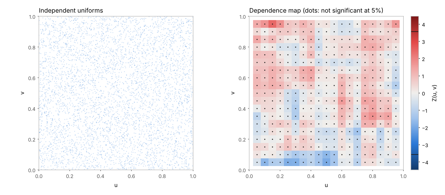
+Classifier: Operating System :: OS Independent
+Classifier: Programming Language :: Python :: 3
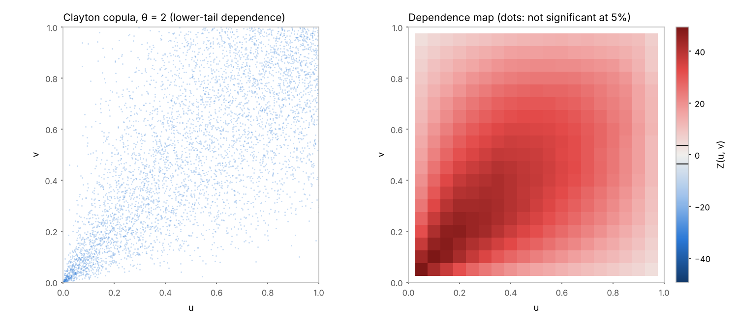
+Classifier: Topic :: Scientific/Engineering :: Mathematics
+Classifier: Topic :: Scientific/Engineering :: Visualization
+Requires-Python: >=3.9
+Description-Content-Type: text/markdown
+License-File: LICENSE
+Requires-Dist: numpy>=1.22
+Requires-Dist: scipy>=1.8
+Requires-Dist: matplotlib>=3.5
+Provides-Extra: pandas
+Requires-Dist: pandas>=1.4; extra == "pandas"
+Provides-Extra: test
+Requires-Dist: pytest>=7; extra == "test"
+Requires-Dist: pandas>=1.4; extra == "test"
+Dynamic: license-file
+
+# dependence-maps
+
+Dependence maps: a graphical tool for visualizing dependence between two scalar random variables.
+
+A dependence map shows, on a grid of quantile levels (u, v), the signed and standardized deviation of the empirical copula from the independence copula. It indicates where in the joint distribution two variables depart from independence: around the median, in the joint upper or lower tail, or in the off-diagonal corners. The method was presented at CFE-CMStatistics 2024 ([slides](https://github.com/Brainologist/dependence-maps/blob/main/docs/CFE2024_dependence_maps_slides.pdf)).
+
+![Dependence map of simulated hourly temperature and power price](https://raw.githubusercontent.com/Brainologist/dependence-maps/main/docs/images/example4_u_shape.png)
+
+## Installation
+
+```bash
+pip install dependence-maps
+```
+
+The package is imported as `depmaps` (the name `depmap` was already taken on PyPI). It requires Python 3.9 or later, NumPy, SciPy and Matplotlib. pandas is optional and is only needed for `to_frame()` and the `data=` argument:
+
+```bash
+pip install "dependence-maps[pandas]"
+```
+
+For the development version, clone [the repository](https://github.com/Brainologist/dependence-maps) and run `pip install -e ".[test]"`, then `pytest`.
+
+## Quickstart
+
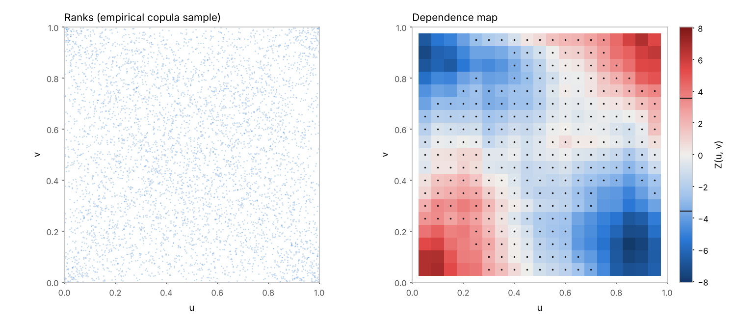
+The data below follow a Student t copula with zero correlation and three degrees of freedom. The correlation coefficient is close to zero, but the two variables are far from independent.
+
+```python
+import matplotlib.pyplot as plt
+import depmaps as dpm
+from depmaps.simulate import t_copula
+
+uv = t_copula(5000, rho=0.0, df=3, rng=1)
+x, y = uv[:, 0], uv[:, 1]
+
+dm = dpm.dependence_map(x, y, grid=19)   # quantile levels 0.05, ..., 0.95
+dm.simultaneous_band(alpha=0.05)          # critical value for max |Z| over the grid
+print(dm.global_pvalue)                   # p-value of the test of independence
+
+dm.plot()                                 # dots mark cells that are not significant
+plt.show()
+```
+
+![Student t copula with zero correlation](https://raw.githubusercontent.com/Brainologist/dependence-maps/main/docs/images/quickstart.png)
+
+`x` and `y` can be NumPy arrays, lists or pandas Series of equal length. Pairs with a missing value are dropped. Columns of a DataFrame can be passed by name, as in `dpm.dependence_map("load", "price", data=df)`.
+
+## Examples from the CFE 2024 talk
+
+[`examples/cfe2024_examples.py`](https://github.com/Brainologist/dependence-maps/blob/main/examples/cfe2024_examples.py) reproduces the examples of the talk with simulated data and writes the figures below. Slide numbers refer to the [slides](https://github.com/Brainologist/dependence-maps/blob/main/docs/CFE2024_dependence_maps_slides.pdf).
+
+### Linear dependence (Example 1, slides 3 and 19–20)
+
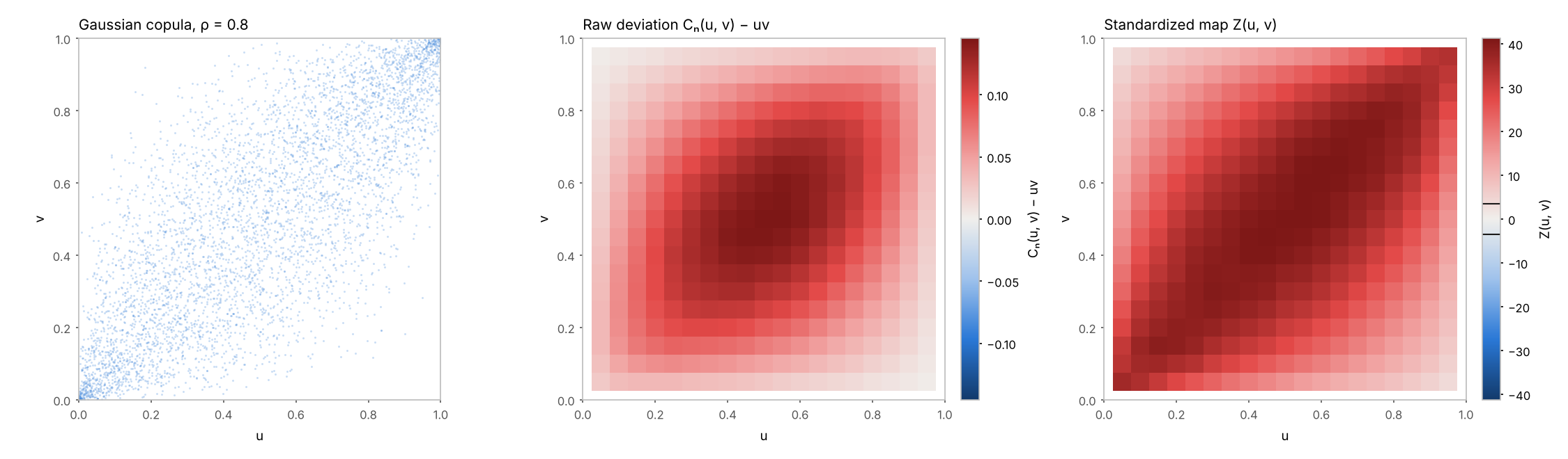
+Gaussian copula with ρ = 0.8. The raw deviation Cₙ(u, v) − uv (middle panel) is largest at the median, but only because it must vanish at the edges of the unit square. The standardized map (right) shows dependence of similar strength along the whole diagonal.
+
+![Gaussian copula: raw and standardized maps](https://raw.githubusercontent.com/Brainologist/dependence-maps/main/docs/images/example1_gaussian.png)
+
+### Tail dependence without correlation (Example 2, slides 4 and 21–23)
+
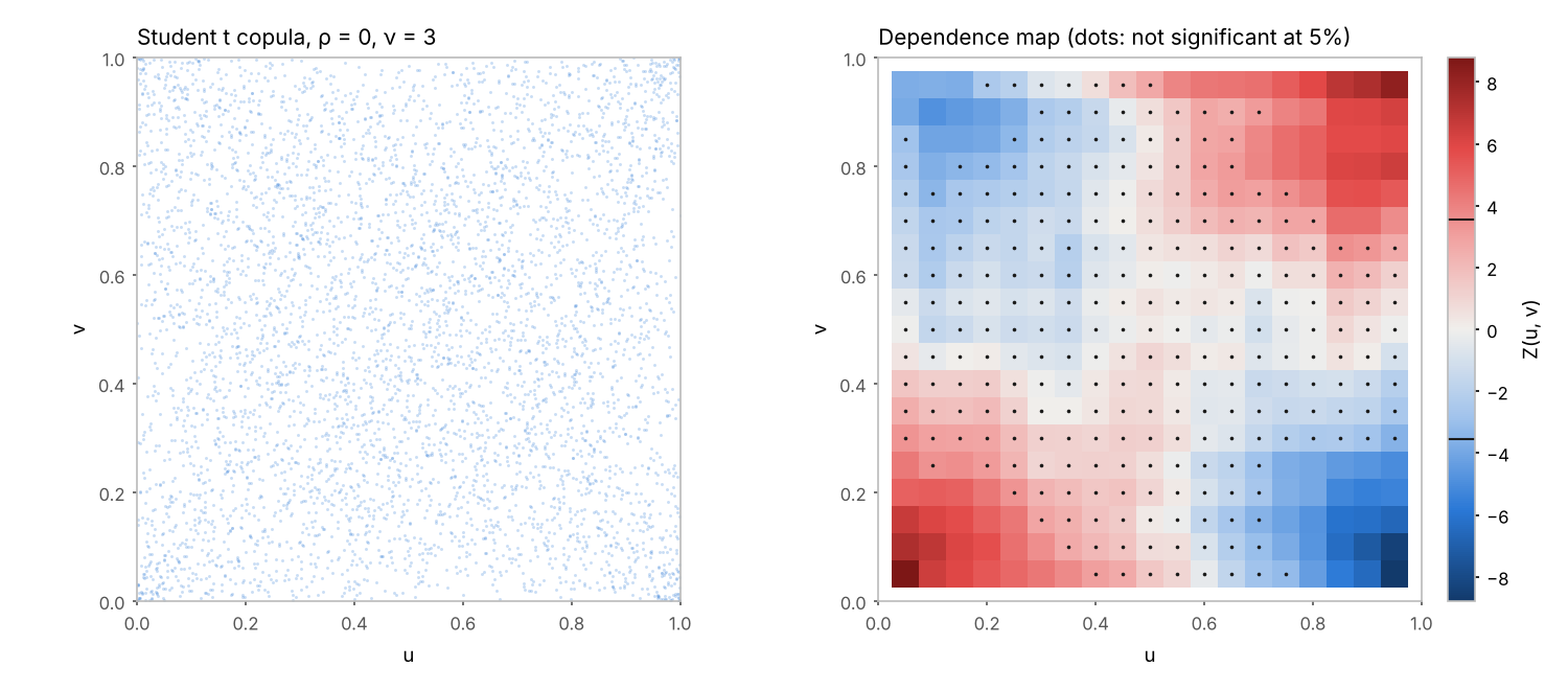
+Student t copula with ρ = 0 and three degrees of freedom. Joint extremes of the same sign occur more often than under independence (red corners) and extremes of opposite sign less often (blue corners). The centre of the map shows nothing.
+
+![Student t copula](https://raw.githubusercontent.com/Brainologist/dependence-maps/main/docs/images/example2_t_tail_dependence.png)
+
+### Independence (slides 16–18)
+
+Even under independence the map shows streaks, since neighbouring cells are strongly correlated. Significance is therefore judged against a simultaneous critical value, about 3.5 for a 19×19 grid, rather than the pointwise 1.96.
+
+![Independence](https://raw.githubusercontent.com/Brainologist/dependence-maps/main/docs/images/example3_independence.png)
+
+### U-shaped dependence in a time series (compare slides 31–33)
+
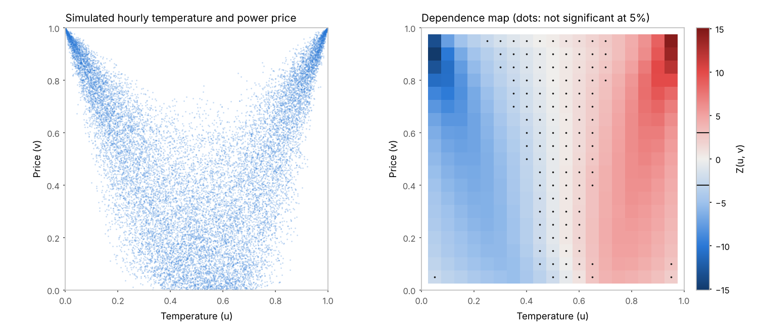
+Simulated hourly temperature and power price, with the price rising in both cold and hot weather, much as in the temperature and day-ahead price application of the talk. The map is blue on the cold side and red on the hot side, whereas a map of absolute deviations would show both sides as a single region of strong dependence. Both series are strongly autocorrelated, so the map is computed with `serial="hac"`. This is the figure at the top of the page.
+
+### Lower-tail dependence (compare slides 34–36)
+
+Clayton copula with θ = 2, where dependence is strongest in the joint lower tail. The load and day-ahead price application of the talk shows a similar asymmetry.
+
+![Clayton copula](https://raw.githubusercontent.com/Brainologist/dependence-maps/main/docs/images/example5_lower_tail.png)
+
+## The statistic
+
+For a sample (X₁, Y₁), …, (Xₙ, Yₙ) with empirical copula Cₙ, the map is
+
+    Z(u, v) = √n (Cₙ(u, v) − uv) / √(u(1 − u) v(1 − v)).
+
+When there are ties, u and v are replaced by the largest attainable marginal levels not exceeding them, which keeps the statistic exact.
+
+The map is intuitive and easy to read since:
+
+1. Z(u, v) is a statistic for a 2×2 table. If X is dichotomized at its u-quantile and Y at its v-quantile, then Z(u, v) = √n φ(u, v), where φ is the phi coefficient of the resulting table, and Z² is its Pearson χ² statistic. φ does not depend on the sample size and is available as `dm.phi`. Note, however, that the margins of the table bound |φ| from above. The bound equals 1 on the diagonal u = v but falls quickly away from it, and at (0.1, 0.9) φ cannot exceed 1/9 even under perfect dependence. `dm.phi_rel` = φ/φ_max corrects for this and equals ±1 everywhere under perfect positive or negative dependence.
+2. Under independence and i.i.d. sampling, Z(u, v) is asymptotically N(0, 1) at every point, and the map as a whole converges to a Gaussian field with covariance ρ(u, u′)ρ(v, v′), where ρ(s, t) = (s∧t − st)/√(s(1 − s)t(1 − t)). This covariance contains no unknown quantities, so simultaneous critical values can be obtained by simulation, without resampling. Continuous margins are not required.
+3. The sign carries information. Red cells indicate positive quadrant dependence at (u, v), meaning that the joint lower and joint upper orthants contain more observations than under independence, while blue cells indicate the opposite. A map of |Z| cannot distinguish the two and shows a U-shaped relationship as a single region of strong dependence.
+
+The raw deviation Cₙ − uv is also available (`which="raw"`), but we do not recommend using it on its own. By the Fréchet bounds it tends to zero at the edges of the unit square regardless of the strength of dependence, which exaggerates dependence near the median.
+
+## Usage
+
+```python
+import depmaps as dpm
+
+dm = dpm.dependence_map(x, y, grid=19)          # levels 0.05, ..., 0.95
+dm.simultaneous_band(alpha=0.05)                 # critical value for max |Z|
+dm.plot()                                        # signed map; dots mark non-significant cells
+dm.plot(which="phi_rel")                         # effect size relative to its bound
+dm.to_frame()                                    # map as a table (needs pandas)
+dm.global_pvalue                                 # sup-norm test of independence
+
+# serially dependent data
+dm = dpm.dependence_map("load", "price", data=df, grid=19,
+                        serial="hac")               # lag by the Andrews (1991) rule
+dm = dpm.dependence_map("load", "price", data=df, grid=19,
+                        serial="hac", max_lag=168)  # or a fixed lag
+dm.simultaneous_band(method="gaussian")          # HAC Gaussian null
+dm.simultaneous_band(method="shift")             # circular shifts of Y
+```
+
+## Inference
+
+Simultaneous critical values can be computed in four ways:
+
+| method | null distribution | valid for |
+|---|---|---|
+| `gaussian` | Gaussian field with known covariance | i.i.d. data |
+| `gaussian` with `serial="hac"` | Gaussian field with covariance Σ_h w_h Γ_A(h) ⊗ Γ_B(h), estimated | stationary, weakly dependent series |
+| `permutation` | random permutations of Y | i.i.d. data, exact under ties |
+| `shift` | random circular shifts of Y | stationary series |
+
+The HAC Gaussian null uses a dense covariance matrix over all pairs of grid cells and is therefore limited to 2,500 cells (a 49×49 grid). For finer grids, use `shift`.
+
+Under serial dependence, the pointwise null variance of √n(Cₙ − uv) equals Σ_h γ_A(h)γ_B(h), where A_t = 1{U_t ≤ u} − u and B_t = 1{V_t ≤ v} − v are centred indicator series. With `serial="hac"`, the ratio κ(u, v) of this long-run variance to its i.i.d. counterpart is estimated with Bartlett weights and the map reports Z/√κ. The truncation lag is chosen by the AR(1) plug-in rule of Andrews (1991) applied to A_t B_t. The Newey–West rule of thumb is available as `max_lag="nw"`, but it is much too short for persistent series such as hourly prices. For persistent and seasonal series κ can be large and may keep growing with the lag, so results should be reported for several lags.
+
+## Tests
+
+Running `pytest` checks both the code and the underlying theory. Among other things, the tests verify that:
+
+- the raw deviation at the centre of the Gaussian copula equals arcsin(ρ)/2π, and Z² equals the χ² statistic of the corresponding 2×2 table;
+- the statistic remains exact under ties and is standard normal under independence;
+- the simultaneous band has the correct size, and Gaussian and permutation critical values agree;
+- the map detects dependence that is confined to the tails;
+- for AR(1) series, the HAC correction restores unit null variance and gives a band of approximately correct size;
+- φ/φ_max equals ±1 under perfect dependence, and the plug-in lag increases with persistence;
+- the copula samplers have uniform margins and the correct Kendall's τ;
+- invalid input (grid and lag arguments, misaligned indexes) is rejected with a clear error.
+
+## Citing
+
+If you use the package, please cite:
+
+> Medovikov, I. (2024). *Dependence Maps: A Graphical Tool for Visualizing Dependence.* 18th International Conference on Computational and Financial Econometrics (CFE-CMStatistics 2024), King's College London, 14–16 December 2024.
+
+The repository includes a `CITATION.cff` file, which GitHub uses for its "Cite this repository" button.
+
+## License
+
+MIT; see [`LICENSE`](https://github.com/Brainologist/dependence-maps/blob/main/LICENSE).

dependence_maps-0.1.1.dist-info/RECORD

@@ -0,0 +1,10 @@
+dependence_maps-0.1.1.dist-info/licenses/LICENSE,sha256=hfjQWbvhjvxQrzxohAWnD2h8--vxE_EbzqTWCqIi8-E,1071
+depmaps/__init__.py,sha256=gGiZTWYKMy28-EJNlKWRhJRaYJBhwH6NGFdupcwjQOI,635
+depmaps/core.py,sha256=Iz4ofn7VfSpHfehJDqFfq07HDuGsAti-8DyzuaUl1Go,14778
+depmaps/inference.py,sha256=8gKU_qwmL1aDYSJvhuZVLIHH-qnoSjFdfRoNH6K5nQU,6112
+depmaps/plotting.py,sha256=5MngEhh5LJCWyV24uIUFx5Z_0Ho2nJ2Zsz45cRx-hZ0,6457
+depmaps/simulate.py,sha256=IvU11dypz2iKWiFp2mUpic8QaE0-HpQPrpvvUxPkRYw,1266
+dependence_maps-0.1.1.dist-info/METADATA,sha256=JbfA4sq1wUnPT2AnXHJ4Jai_orgj5IFWoWwOqV8Y-5A,11847
+dependence_maps-0.1.1.dist-info/WHEEL,sha256=mOdXR9C3wMVov7cSY8PY-XCzo3SmmWCHvGQr5csJoao,91
+dependence_maps-0.1.1.dist-info/top_level.txt,sha256=LlKEz93XkIYGTB-8GSX8PKBznPWyQG1PiW8kqF8lbNU,8
+dependence_maps-0.1.1.dist-info/RECORD,,

dependence_maps-0.1.1.dist-info/WHEEL

@@ -0,0 +1,5 @@
+Wheel-Version: 1.0
+Generator: setuptools (84.2.1)
+Root-Is-Purelib: true
+Tag: py3-none-any
+

dependence_maps-0.1.1.dist-info/licenses/LICENSE

@@ -0,0 +1,21 @@
+MIT License
+
+Copyright (c) 2026 Ivan Medovikov
+
+Permission is hereby granted, free of charge, to any person obtaining a copy
+of this software and associated documentation files (the "Software"), to deal
+in the Software without restriction, including without limitation the rights
+to use, copy, modify, merge, publish, distribute, sublicense, and/or sell
+copies of the Software, and to permit persons to whom the Software is
+furnished to do so, subject to the following conditions:
+
+The above copyright notice and this permission notice shall be included in all
+copies or substantial portions of the Software.
+
+THE SOFTWARE IS PROVIDED "AS IS", WITHOUT WARRANTY OF ANY KIND, EXPRESS OR
+IMPLIED, INCLUDING BUT NOT LIMITED TO THE WARRANTIES OF MERCHANTABILITY,
+FITNESS FOR A PARTICULAR PURPOSE AND NONINFRINGEMENT. IN NO EVENT SHALL THE
+AUTHORS OR COPYRIGHT HOLDERS BE LIABLE FOR ANY CLAIM, DAMAGES OR OTHER
+LIABILITY, WHETHER IN AN ACTION OF CONTRACT, TORT OR OTHERWISE, ARISING FROM,
+OUT OF OR IN CONNECTION WITH THE SOFTWARE OR THE USE OR OTHER DEALINGS IN THE
+SOFTWARE.

dependence_maps-0.1.1.dist-info/top_level.txt

@@ -0,0 +1 @@
+depmaps

depmaps/__init__.py

@@ -0,0 +1,21 @@
+"""Dependence maps: signed standardized deviations of the empirical copula from independence."""
+from .core import DependenceMap, dependence_map, make_grid, pseudo_obs, default_max_lag, andrews_max_lag
+from .inference import null_covariance, null_max_distribution, simultaneous_band
+from .plotting import DEPMAP_CMAP, plot_map, rank_scatter
+
+__all__ = [
+    "DependenceMap",
+    "dependence_map",
+    "make_grid",
+    "pseudo_obs",
+    "default_max_lag",
+    "andrews_max_lag",
+    "simultaneous_band",
+    "null_max_distribution",
+    "null_covariance",
+    "plot_map",
+    "rank_scatter",
+    "DEPMAP_CMAP",
+]
+
+__version__ = "0.1.1"

depmaps/core.py

@@ -0,0 +1,381 @@
+"""Core computation of dependence maps.
+
+A dependence map evaluates, on a grid of quantile levels (u, v), the signed
+standardized deviation of the empirical copula from the independence copula
+
+    Z(u, v) = sqrt(n) * (C_n(a, b) - a b) / sqrt(a (1 - a) b (1 - b)),
+
+where a = a(u) and b = b(v) are the marginal proportions actually attained
+when X is cut at its empirical u-quantile and Y at its empirical v-quantile.
+Without ties a = floor(n u) / n -> u; with ties a is the largest attainable
+level not exceeding u, which keeps the statistic exact. The Gaussian limit
+below does not require continuous margins.
+
+Equivalently, Z(u, v) = sqrt(n) * phi(u, v), where phi is the phi coefficient
+of the 2x2 contingency table obtained by dichotomizing X at its u-quantile and
+Y at its v-quantile, and Z(u, v)^2 is that table's Pearson chi-square
+statistic. Under independence (i.i.d. sampling) Z(u, v) is asymptotically
+N(0, 1) pointwise, and the field {Z(u, v)} converges to a centred Gaussian
+field with covariance
+
+    rho_a(u, u') * rho_b(v, v'),   rho(s, t) = (s ^ t - s t) / sqrt(s(1-s) t(1-t)),
+
+i.e. a normalized tied-down Brownian pillow.
+
+For serially dependent observations the pointwise null variance of
+sqrt(n)(C_n - ab) is sum_h gamma_A(h) gamma_B(h), where A_t, B_t are the
+centred indicator series. ``serial="hac"`` estimates the ratio of this
+long-run variance to the i.i.d. variance with Bartlett weights and rescales Z.
+"""
+from __future__ import annotations
+
+from dataclasses import dataclass, field
+from typing import Optional, Sequence, Tuple, Union
+
+import numpy as np
+
+GridSpec = Union[int, Sequence[float], np.ndarray]
+
+
+# ---------------------------------------------------------------------------
+# helpers
+# ---------------------------------------------------------------------------
+
+def pseudo_obs(x: np.ndarray) -> np.ndarray:
+    """Empirical CDF values F_n(x_i) = #{j : x_j <= x_i} / n ("max" ranks / n).
+
+    Ties receive the same value, the largest rank in their group, so that
+    {F_n(X_i) <= u} is exactly the event {X_i <= empirical u-quantile}.
+    """
+    x = np.asarray(x, dtype=float)
+    n = x.shape[0]
+    order = np.sort(x)
+    return np.searchsorted(order, x, side="right") / n
+
+
+def make_grid(grid: GridSpec) -> np.ndarray:
+    """Quantile levels strictly inside (0, 1).
+
+    An integer g gives the equispaced interior grid (1, ..., g) / (g + 1).
+    """
+    if np.isscalar(grid):
+        if isinstance(grid, (bool, np.bool_)) or not float(grid).is_integer():
+            raise ValueError(
+                f"grid={grid!r}: a scalar grid must be a whole number of levels; "
+                "pass quantile levels as a list or array, e.g. grid=[0.25, 0.75]"
+            )
+        g = int(grid)
+        if g < 1:
+            raise ValueError("grid size must be >= 1")
+        return np.arange(1, g + 1) / (g + 1)
+    levels = np.sort(np.asarray(grid, dtype=float).ravel())
+    if np.any(levels <= 0) or np.any(levels >= 1):
+        raise ValueError("grid levels must lie strictly inside (0, 1)")
+    return levels
+
+
+def _indicators(F: np.ndarray, levels: np.ndarray) -> np.ndarray:
+    """n x g matrix of 1{F_n(X_i) <= level_k} as float64."""
+    return (F[:, None] <= levels[None, :] + 1e-12).astype(float)
+
+
+def _acf_columns(M: np.ndarray, max_lag: int) -> np.ndarray:
+    """Autocorrelations of each (centred) column of M for lags 1..max_lag.
+
+    Returns an array of shape (max_lag, g). Uses FFT; columns with zero
+    variance get zero autocorrelation.
+    """
+    n, g = M.shape
+    Mc = M - M.mean(axis=0, keepdims=True)
+    nfft = 1 << int(np.ceil(np.log2(2 * n - 1)))
+    f = np.fft.rfft(Mc, n=nfft, axis=0)
+    ac = np.fft.irfft(f * np.conj(f), n=nfft, axis=0)[: max_lag + 1]
+    var = ac[0]
+    with np.errstate(invalid="ignore", divide="ignore"):
+        r = np.where(var > 0, ac[1:] / var, 0.0)
+    return r
+
+
+def default_max_lag(n: int) -> int:
+    """Newey-West (1994) style rule of thumb, floor(4 (n/100)^(2/9))."""
+    return int(np.floor(4 * (n / 100.0) ** (2.0 / 9.0)))
+
+
+def andrews_max_lag(A: np.ndarray, B: np.ndarray) -> int:
+    """Andrews (1991) AR(1) plug-in truncation lag for the Bartlett kernel.
+
+    The long-run variance of interest is that of the products A_t B_t, whose
+    first-order autocorrelation under independence is rho_A * rho_B. The
+    plug-in uses the median of these products over the grid:
+    L = 1.1447 (alpha n)^(1/3), alpha = 4 rho^2 / (1 - rho^2)^2.
+    """
+    n = A.shape[0]
+    rA = _acf_columns(A, 1)[0]
+    rB = _acf_columns(B, 1)[0]
+    rho = float(np.median(np.abs(np.outer(rA, rB))))
+    rho = min(rho, 0.99)
+    alpha = 4.0 * rho**2 / (1.0 - rho**2) ** 2
+    L = int(np.ceil(1.1447 * (alpha * n) ** (1.0 / 3.0)))
+    return max(1, min(L, n // 4))
+
+
+def bartlett_weights(max_lag: int) -> np.ndarray:
+    h = np.arange(1, max_lag + 1)
+    return 1.0 - h / (max_lag + 1.0)
+
+
+# ---------------------------------------------------------------------------
+# result container
+# ---------------------------------------------------------------------------
+
+@dataclass
+class DependenceMap:
+    """Result of :func:`dependence_map`.
+
+    Attributes
+    ----------
+    u, v : nominal quantile levels kept on each axis (after dropping levels
+        that collapse onto the same attainable proportion because of ties).
+    a, b : attained marginal proportions at those levels (equal u, v up to
+        O(1/n) without ties). Maps are plotted against ``a`` and ``b``.
+    n : number of complete observations used.
+    raw : signed raw deviation C_n(a, b) - a b, shape (len(a), len(b)).
+        Rows index X levels, columns index Y levels.
+    z_iid : sqrt(n) * raw / sqrt(a(1-a) b(1-b)), the i.i.d. standardization.
+    kappa : long-run variance inflation factor (None unless serial="hac").
+    z : the map to read; z_iid / sqrt(kappa) if serial correction is on.
+    """
+
+    u: np.ndarray
+    v: np.ndarray
+    a: np.ndarray
+    b: np.ndarray
+    n: int
+    raw: np.ndarray
+    z_iid: np.ndarray
+    kappa: Optional[np.ndarray] = None
+    max_lag: Optional[int] = None
+    xlabel: str = "X"
+    ylabel: str = "Y"
+    # kept for inference (indicator matrices); not part of the public repr
+    _A: Optional[np.ndarray] = field(default=None, repr=False)
+    _B: Optional[np.ndarray] = field(default=None, repr=False)
+    critical_value: Optional[float] = None
+    critical_method: Optional[str] = None
+    alpha: Optional[float] = None
+    global_pvalue: Optional[float] = None
+
+    @property
+    def z(self) -> np.ndarray:
+        if self.kappa is None:
+            return self.z_iid
+        return self.z_iid / np.sqrt(self.kappa)
+
+    @property
+    def phi(self) -> np.ndarray:
+        """Effect-size map: the phi coefficient of each dichotomized 2x2 table.
+
+        phi = raw / sqrt(a(1-a) b(1-b)) = z_iid / sqrt(n). Comparable across
+        samples of different size, in [-1, 1].
+        """
+        return self.raw / np.sqrt(np.outer(self.a * (1 - self.a), self.b * (1 - self.b)))
+
+    @property
+    def phi_max(self) -> np.ndarray:
+        """Largest |phi| attainable given the margins, for the sign of each cell.
+
+        For phi >= 0 the bound is sqrt(min(a,b)(1-max(a,b)) / (max(a,b)(1-min(a,b))));
+        for phi < 0 it is sqrt(ab / ((1-a)(1-b))) when a + b <= 1 and
+        sqrt((1-a)(1-b) / (ab)) otherwise. Off the diagonal the bound is well
+        below one, so phi maps fade away from the diagonal even under perfect
+        dependence.
+        """
+        A, B = np.meshgrid(self.a, self.b, indexing="ij")
+        lo, hi = np.minimum(A, B), np.maximum(A, B)
+        pos = np.sqrt(lo * (1 - hi) / (hi * (1 - lo)))
+        neg = np.where(A + B <= 1, np.sqrt(A * B / ((1 - A) * (1 - B))),
+                       np.sqrt((1 - A) * (1 - B) / (A * B)))
+        return np.where(self.raw >= 0, pos, neg)
+
+    @property
+    def phi_rel(self) -> np.ndarray:
+        """phi / phi_max: phi relative to its attainable bound, in [-1, 1].
+
+        Equals +1 everywhere under comonotonicity and -1 under
+        countermonotonicity, regardless of (u, v).
+        """
+        return self.phi / self.phi_max
+
+    @property
+    def pvalues(self) -> np.ndarray:
+        """Pointwise two-sided p-values from the N(0, 1) approximation."""
+        from scipy.stats import norm
+
+        return 2.0 * norm.sf(np.abs(self.z))
+
+    @property
+    def max_abs_z(self) -> float:
+        return float(np.nanmax(np.abs(self.z)))
+
+    def significant(self) -> np.ndarray:
+        """Boolean mask of cells exceeding the simultaneous critical value."""
+        if self.critical_value is None:
+            raise ValueError("call simultaneous_band(...) first")
+        return np.abs(self.z) > self.critical_value
+
+    def to_frame(self, which: str = "z"):
+        """Return the map as a pandas DataFrame (rows: X levels, cols: Y levels)."""
+        import pandas as pd
+
+        M = {"z": self.z, "z_iid": self.z_iid, "raw": self.raw, "phi": self.phi,
+             "phi_rel": self.phi_rel}[which]
+        return pd.DataFrame(
+            M,
+            index=pd.Index(np.round(self.a, 4), name=f"{self.xlabel} level"),
+            columns=pd.Index(np.round(self.b, 4), name=f"{self.ylabel} level"),
+        )
+
+    def plot(self, **kwargs):
+        from .plotting import plot_map
+
+        return plot_map(self, **kwargs)
+
+    def simultaneous_band(self, **kwargs) -> float:
+        from .inference import simultaneous_band
+
+        return simultaneous_band(self, **kwargs)
+
+
+# ---------------------------------------------------------------------------
+# main entry point
+# ---------------------------------------------------------------------------
+
+def _as_array_and_label(obj, default):
+    name = getattr(obj, "name", None)
+    return np.asarray(obj, dtype=float).ravel(), (str(name) if name is not None else default)
+
+
+def dependence_map(
+    x,
+    y=None,
+    grid: Union[GridSpec, Tuple[GridSpec, GridSpec]] = 19,
+    *,
+    data=None,
+    serial: Optional[str] = None,
+    max_lag: Union[int, str, None] = "auto",
+    keep_indicators: bool = True,
+) -> DependenceMap:
+    """Compute a signed, standardized dependence map.
+
+    Parameters
+    ----------
+    x, y : array-like of equal length, or column names when ``data`` is given.
+        Pairs with a missing value in either coordinate are dropped.
+    grid : int, list/array of levels, or a tuple ``(x_grid, y_grid)`` of these.
+        Default 19 gives levels 0.05, 0.10, ..., 0.95.
+    data : optional DataFrame from which ``x`` and ``y`` are taken.
+    serial : None (i.i.d. standardization) or "hac" (Bartlett long-run
+        variance correction for serially dependent data).
+    max_lag : truncation lag for ``serial="hac"``. "auto" (default) uses the
+        Andrews (1991) AR(1) plug-in rule (:func:`andrews_max_lag`); "nw"
+        uses the Newey-West rule of thumb (:func:`default_max_lag`), which is
+        far too short for persistent data such as hourly prices; an integer
+        sets the lag directly. Because the long-run variance of seasonal
+        series may not settle as the lag grows, results should be reported
+        for several lags.
+    keep_indicators : store indicator matrices, needed by
+        :func:`depmaps.simultaneous_band` and the permutation/shift methods.
+    """
+    if data is not None:
+        xlab, ylab = str(x), str(y)
+        x, y = data[x], data[y]
+    if y is None:
+        raise ValueError("y is required")
+    ix, iy = getattr(x, "index", None), getattr(y, "index", None)
+    if hasattr(ix, "equals") and hasattr(iy, "equals") and not ix.equals(iy):
+        raise ValueError("x and y have different indexes; align them before calling")
+    xv, xlab_ = _as_array_and_label(x, "X")
+    yv, ylab_ = _as_array_and_label(y, "Y")
+    if data is None:
+        xlab, ylab = xlab_, ylab_
+    if xv.shape != yv.shape:
+        raise ValueError("x and y must have the same length")
+
+    ok = np.isfinite(xv) & np.isfinite(yv)
+    n_dropped = int((~ok).sum())
+    if serial is not None and n_dropped:
+        import warnings
+
+        warnings.warn(
+            f"{n_dropped} incomplete observations dropped; the remaining series is "
+            "treated as contiguous when estimating serial dependence",
+            stacklevel=2,
+        )
+    xv, yv = xv[ok], yv[ok]
+    n = xv.shape[0]
+    if n < 10:
+        raise ValueError("need at least 10 complete observations")
+
+    if isinstance(grid, tuple):
+        if len(grid) != 2:
+            raise ValueError("a tuple grid must be (x_grid, y_grid); pass levels as a list or array")
+        gx, gy = make_grid(grid[0]), make_grid(grid[1])
+    else:
+        gx = gy = make_grid(grid)
+
+    U, V = pseudo_obs(xv), pseudo_obs(yv)
+    A, B = _indicators(U, gx), _indicators(V, gy)
+    a, b = A.mean(axis=0), B.mean(axis=0)
+
+    # drop levels that are degenerate (a in {0, 1}) or duplicate because of ties
+    def _keep(p):
+        valid = (p > 0) & (p < 1)
+        idx = np.flatnonzero(valid)
+        _, first = np.unique(np.round(p[idx], 12), return_index=True)
+        return np.sort(idx[first])
+
+    kx, ky = _keep(a), _keep(b)
+    if kx.size == 0 or ky.size == 0:
+        raise ValueError("no non-degenerate grid levels (variable is constant?)")
+    gx, gy, A, B, a, b = gx[kx], gy[ky], A[:, kx], B[:, ky], a[kx], b[ky]
+
+    p11 = (A.T @ B) / n
+    raw = p11 - np.outer(a, b)
+    scale = np.sqrt(np.outer(a * (1 - a), b * (1 - b)))
+    z_iid = np.sqrt(n) * raw / scale
+
+    kappa = None
+    L = None
+    if serial is None and max_lag not in (None, "auto"):
+        import warnings
+
+        warnings.warn("max_lag is ignored unless serial='hac'", stacklevel=2)
+    if serial is not None:
+        if serial != "hac":
+            raise ValueError("serial must be None or 'hac'")
+        if max_lag is None or max_lag == "auto":
+            L = andrews_max_lag(A, B)
+        elif max_lag == "nw":
+            L = default_max_lag(n)
+        elif isinstance(max_lag, (int, np.integer)) and not isinstance(max_lag, bool):
+            L = int(max_lag)
+            if L < 0:
+                raise ValueError("max_lag must be non-negative")
+        else:
+            raise ValueError("max_lag must be 'auto', 'nw' or a non-negative integer")
+        if L >= n:
+            raise ValueError("max_lag must be smaller than the number of observations")
+        if L >= 1:
+            w = bartlett_weights(L)
+            RA = _acf_columns(A, L)  # (L, gx)
+            RB = _acf_columns(B, L)  # (L, gy)
+            kappa = 1.0 + 2.0 * (RA * w[:, None]).T @ RB
+            kappa = np.maximum(kappa, 1e-3)
+        else:
+            kappa = np.ones_like(z_iid)
+
+    return DependenceMap(
+        u=gx, v=gy, a=a, b=b, n=n, raw=raw, z_iid=z_iid, kappa=kappa,
+        max_lag=L, xlabel=xlab, ylabel=ylab,
+        _A=A if keep_indicators else None, _B=B if keep_indicators else None,
+    )

depmaps/inference.py

@@ -0,0 +1,165 @@
+"""Simultaneous inference for dependence maps.
+
+All methods calibrate the distribution of max_{(u,v) in grid} |Z(u, v)| under
+the null of independence between X and Y, giving a critical value c_alpha
+such that, under the null, P(max |Z| > c_alpha) ~= alpha. Cells with
+|Z| > c_alpha are significant with family-wise error rate alpha.
+
+Methods
+-------
+gaussian     Simulate the limiting Gaussian field. For i.i.d. data its
+             covariance is the Kronecker product of normalized Brownian-bridge
+             kernels in the attained levels (no unknowns). With a HAC-corrected
+             map (serial="hac") the covariance is
+             sum_h w_h Gamma_A(h) (x) Gamma_B(h), estimated from the
+             indicator series, then normalized to unit diagonal.
+permutation  Randomly permute Y relative to X. Exact for i.i.d. data and
+             handles ties; invalid for serially dependent data.
+shift        Random circular shifts of Y relative to X (toroidal shifts).
+             Preserves each series' own serial dependence and breaks the
+             cross-dependence; the natural resampling null for stationary
+             time series.
+"""
+from __future__ import annotations
+
+import warnings
+from typing import Optional
+
+import numpy as np
+
+from .core import DependenceMap, bartlett_weights
+
+
+MAX_HAC_CELLS = 2500
+
+
+def _bridge_corr(p: np.ndarray) -> np.ndarray:
+    s = np.sqrt(p * (1 - p))
+    return (np.minimum.outer(p, p) - np.outer(p, p)) / np.outer(s, s)
+
+
+def _psd_factor(S: np.ndarray) -> np.ndarray:
+    """Symmetric square-root factor of a (nearly) PSD matrix."""
+    S = 0.5 * (S + S.T)
+    w, V = np.linalg.eigh(S)
+    w = np.clip(w, 0.0, None)
+    return V * np.sqrt(w)
+
+
+def _lagged_cov(Mc: np.ndarray, h: int) -> np.ndarray:
+    n = Mc.shape[0]
+    if h == 0:
+        return Mc.T @ Mc / n
+    return Mc[:-h].T @ Mc[h:] / n
+
+
+def null_covariance(dm: DependenceMap) -> np.ndarray:
+    """Null correlation matrix of vec(Z) (row-major over the grid)."""
+    if dm.kappa is None:
+        return np.kron(_bridge_corr(dm.a), _bridge_corr(dm.b))
+    cells = dm.a.size * dm.b.size
+    if cells > MAX_HAC_CELLS:
+        raise ValueError(
+            f"the HAC Gaussian null needs a dense {cells}x{cells} covariance matrix; "
+            f"use a grid with at most {MAX_HAC_CELLS} cells (e.g. 49x49) or method='shift'"
+        )
+    if dm._A is None or dm._B is None:
+        raise ValueError("map was computed with keep_indicators=False")
+    Ac = dm._A - dm.a
+    Bc = dm._B - dm.b
+    S = np.kron(_lagged_cov(Ac, 0), _lagged_cov(Bc, 0))
+    for h, w in zip(range(1, dm.max_lag + 1), bartlett_weights(dm.max_lag)):
+        GA, GB = _lagged_cov(Ac, h), _lagged_cov(Bc, h)
+        S += w * (np.kron(GA, GB) + np.kron(GA.T, GB.T))
+    d = np.sqrt(np.clip(np.diag(S), 1e-300, None))
+    return S / np.outer(d, d)
+
+
+def _max_abs_z_from_B(dm: DependenceMap, Bp: np.ndarray) -> float:
+    n = dm.n
+    raw = (dm._A.T @ Bp) / n - np.outer(dm.a, dm.b)
+    z = np.sqrt(n) * raw / np.sqrt(np.outer(dm.a * (1 - dm.a), dm.b * (1 - dm.b)))
+    if dm.kappa is not None:
+        z = z / np.sqrt(dm.kappa)
+    return float(np.max(np.abs(z)))
+
+
+def null_max_distribution(
+    dm: DependenceMap,
+    method: str = "gaussian",
+    n_sim: int = 2000,
+    rng: Optional[np.random.Generator] = None,
+    min_shift: Optional[int] = None,
+) -> np.ndarray:
+    """Draws of max |Z| over the grid under the null of independence."""
+    rng = np.random.default_rng(rng)
+    ga, gb = dm.a.size, dm.b.size
+
+    if method == "gaussian":
+        if dm.kappa is None:
+            La, Lb = _psd_factor(_bridge_corr(dm.a)), _psd_factor(_bridge_corr(dm.b))
+            out = np.empty(n_sim)
+            chunk = 500
+            for s in range(0, n_sim, chunk):
+                k = min(chunk, n_sim - s)
+                E = rng.standard_normal((k, La.shape[1], Lb.shape[1]))
+                Z = La @ E @ Lb.T
+                out[s : s + k] = np.abs(Z).reshape(k, -1).max(axis=1)
+            return out
+        F = _psd_factor(null_covariance(dm))
+        out = np.empty(n_sim)
+        chunk = 500
+        for s in range(0, n_sim, chunk):
+            k = min(chunk, n_sim - s)
+            Z = rng.standard_normal((k, F.shape[1])) @ F.T
+            out[s : s + k] = np.abs(Z).max(axis=1)
+        return out
+
+    if dm._A is None or dm._B is None:
+        raise ValueError("map was computed with keep_indicators=False")
+
+    if method == "permutation":
+        if dm.kappa is not None:
+            warnings.warn(
+                "permutation destroys serial dependence in Y; use method='shift' "
+                "or 'gaussian' for time series",
+                stacklevel=2,
+            )
+        return np.array(
+            [_max_abs_z_from_B(dm, dm._B[rng.permutation(dm.n)]) for _ in range(n_sim)]
+        )
+
+    if method == "shift":
+        n = dm.n
+        m = n // 10 if min_shift is None else int(min_shift)
+        if not 0 < m < n // 2:
+            raise ValueError("min_shift must be in (0, n/2)")
+        shifts = rng.integers(m, n - m + 1, size=n_sim)
+        return np.array([_max_abs_z_from_B(dm, np.roll(dm._B, s, axis=0)) for s in shifts])
+
+    raise ValueError("method must be 'gaussian', 'permutation' or 'shift'")
+
+
+def simultaneous_band(
+    dm: DependenceMap,
+    alpha: float = 0.05,
+    method: str = "gaussian",
+    n_sim: int = 2000,
+    rng=None,
+    min_shift: Optional[int] = None,
+) -> float:
+    """Simultaneous critical value for |Z| over the grid; stored on ``dm``.
+
+    Also stores ``dm.global_pvalue``: the share of null draws with
+    max |Z| >= the observed max |Z| (a test of independence based on the
+    sup-norm of the standardized empirical copula process over the grid).
+    """
+    if not 0 < alpha < 1:
+        raise ValueError("alpha must lie strictly between 0 and 1")
+    draws = null_max_distribution(dm, method=method, n_sim=n_sim, rng=rng, min_shift=min_shift)
+    c = float(np.quantile(draws, 1 - alpha))
+    dm.critical_value = c
+    dm.critical_method = method
+    dm.alpha = alpha
+    dm.global_pvalue = float((1 + np.sum(draws >= dm.max_abs_z)) / (1 + draws.size))
+    return c

depmaps/plotting.py

@@ -0,0 +1,162 @@
+"""Plotting for dependence maps (matplotlib)."""
+from __future__ import annotations
+
+from typing import Optional
+
+import numpy as np
+import matplotlib.pyplot as plt
+from matplotlib.colors import LinearSegmentedColormap, TwoSlopeNorm
+
+# Diverging blue <-> neutral grey <-> red: negative quadrant dependence is
+# blue, positive is red, independence is the neutral midpoint.
+DEPMAP_CMAP = LinearSegmentedColormap.from_list(
+    "depmap",
+    ["#123a6b", "#2a78d6", "#9fc2ec", "#f0efec", "#f1a3a2", "#e34948", "#7d1716"],
+)
+
+
+def _edges(p: np.ndarray) -> np.ndarray:
+    """Cell edges for non-uniform levels: midpoints, clipped to [0, 1]."""
+    mid = 0.5 * (p[1:] + p[:-1])
+    lo = max(0.0, p[0] - (mid[0] - p[0])) if p.size > 1 else max(0.0, p[0] - 0.05)
+    hi = min(1.0, p[-1] + (p[-1] - mid[-1])) if p.size > 1 else min(1.0, p[0] + 0.05)
+    return np.concatenate([[lo], mid, [hi]])
+
+
+def plot_map(
+    dm,
+    ax: Optional[plt.Axes] = None,
+    *,
+    which: str = "z",
+    absolute: bool = False,
+    style: str = "cells",
+    vmax: Optional[float] = None,
+    show_critical: bool = True,
+    pointwise_level: Optional[float] = None,
+    colorbar: bool = True,
+    xlabel: Optional[str] = None,
+    ylabel: Optional[str] = None,
+    title: Optional[str] = None,
+    cmap=None,
+):
+    """Draw a dependence map.
+
+    X levels run along the horizontal axis and Y levels along the vertical
+    axis, origin at bottom-left (lower tails meet at the origin).
+
+    Parameters
+    ----------
+    which : "z" (default, standardized), "phi" (effect size, Z / sqrt(n)
+        under i.i.d. scaling), "phi_rel" (phi relative to the largest value
+        the margins allow, see ``DependenceMap.phi_max``) or "raw" (C_n - ab).
+    absolute : plot |Z| with a sequential scale instead of the signed map.
+    style : "cells" (one flat cell per grid point; no interpolation) or
+        "contour" (filled contours; smoother, reads like the talk figures).
+    show_critical : mark simultaneous significance (requires
+        ``dm.simultaneous_band()`` to have been called). With style="cells"
+        a small dot is placed on every cell whose |Z| does not exceed the
+        critical value, so the marking follows the grid exactly; with
+        style="contour" the |Z| = c contour is drawn instead.
+    pointwise_level : optionally also outline pointwise significance at this
+        level, e.g. 0.05 -> |Z| > 1.96.
+    """
+    if ax is None:
+        _, ax = plt.subplots(figsize=(5.2, 4.4))
+    maps = {"z": dm.z, "raw": dm.raw, "phi": dm.phi, "phi_rel": dm.phi_rel}
+    if which not in maps:
+        raise ValueError(f"which must be one of {sorted(maps)}")
+    if style == "contour" and (dm.a.size < 2 or dm.b.size < 2):
+        raise ValueError("style='contour' needs at least two grid levels on each axis")
+    M = maps[which].T  # rows -> Y
+    a, b = dm.a, dm.b
+
+    if absolute:
+        M = np.abs(M)
+        vm = vmax or float(np.nanmax(M))
+        cm = cmap or LinearSegmentedColormap.from_list("depmap_abs", ["#f0efec", "#e34948", "#7d1716"])
+        norm = plt.Normalize(0, vm)
+    else:
+        vm = vmax or float(np.nanmax(np.abs(M)))
+        if which == "z" and dm.critical_value is not None:
+            vm = max(vm, 1.25 * dm.critical_value)
+        vm = vm if vm > 0 else 1.0
+        cm = cmap or DEPMAP_CMAP
+        norm = TwoSlopeNorm(vmin=-vm, vcenter=0.0, vmax=vm)
+
+    if style == "cells":
+        mesh = ax.pcolormesh(_edges(a), _edges(b), M, cmap=cm, norm=norm, shading="flat")
+    elif style == "contour":
+        levels = np.linspace(norm.vmin, norm.vmax, 21)
+        mesh = ax.contourf(a, b, M, levels=levels, cmap=cm, norm=norm, extend="both")
+    else:
+        raise ValueError("style must be 'cells' or 'contour'")
+
+    if show_critical and dm.critical_value is not None:
+        Zabs = np.abs(dm.z.T)
+        if style == "cells":
+            jj, ii = np.nonzero(Zabs <= dm.critical_value)
+            ax.scatter(a[ii], b[jj], s=3, color="#1a1a19", linewidths=0, zorder=3)
+        else:
+            ax.contour(a, b, Zabs, levels=[dm.critical_value], colors="#1a1a19",
+                       linewidths=1.2)
+    if which == "z":
+        Zabs = np.abs(dm.z.T)
+        if pointwise_level is not None:
+            from scipy.stats import norm as _n
+
+            ax.contour(a, b, Zabs, levels=[_n.isf(pointwise_level / 2)], colors="#1a1a19",
+                       linewidths=0.8, linestyles=":")
+
+    ax.set_xlim(0, 1)
+    ax.set_ylim(0, 1)
+    ax.set_aspect("equal")
+    ax.set_xticks(np.linspace(0, 1, 6))
+    ax.set_yticks(np.linspace(0, 1, 6))
+    ax.tick_params(length=2, labelsize=8, colors="#555")
+    for s in ax.spines.values():
+        s.set_color("#bbb")
+    ax.set_xlabel(xlabel or f"{dm.xlabel} (quantile level u)", fontsize=9)
+    ax.set_ylabel(ylabel or f"{dm.ylabel} (quantile level v)", fontsize=9)
+    if title:
+        ax.set_title(title, fontsize=10, loc="left")
+
+    if colorbar:
+        cb = plt.colorbar(mesh, ax=ax, fraction=0.046, pad=0.04)
+        lab = {"z": "Z(u, v)", "phi": "φ(u, v)", "phi_rel": "φ / φ_max",
+               "raw": "Cₙ(u, v) − uv"}[which]
+        if absolute:
+            lab = f"|{lab}|"
+        cb.set_label(lab, fontsize=9)
+        cb.ax.tick_params(labelsize=8, length=2)
+        cb.outline.set_edgecolor("#bbb")
+        if which == "z" and dm.critical_value is not None:
+            c = dm.critical_value
+            ticks = [-c, c] if not absolute else [c]
+            for t in ticks:
+                cb.ax.axhline(t, color="#1a1a19", lw=1.0)
+    return ax
+
+
+def rank_scatter(x, y, ax=None, *, s=2, alpha=0.25, xlabel="u", ylabel="v", max_points=20000, rng=0):
+    """Scatter of pseudo-observations (F_n(X), F_n(Y)): the empirical copula sample."""
+    from .core import pseudo_obs
+
+    x = np.asarray(x, float)
+    y = np.asarray(y, float)
+    ok = np.isfinite(x) & np.isfinite(y)
+    U, V = pseudo_obs(x[ok]), pseudo_obs(y[ok])
+    if U.size > max_points:
+        idx = np.random.default_rng(rng).choice(U.size, max_points, replace=False)
+        U, V = U[idx], V[idx]
+    if ax is None:
+        _, ax = plt.subplots(figsize=(4.4, 4.4))
+    ax.scatter(U, V, s=s, alpha=alpha, color="#2a78d6", linewidths=0)
+    ax.set_xlim(0, 1)
+    ax.set_ylim(0, 1)
+    ax.set_aspect("equal")
+    ax.set_xlabel(xlabel, fontsize=9)
+    ax.set_ylabel(ylabel, fontsize=9)
+    ax.tick_params(length=2, labelsize=8, colors="#555")
+    for sp in ax.spines.values():
+        sp.set_color("#bbb")
+    return ax

depmaps/simulate.py

@@ -0,0 +1,34 @@
+"""Copula samplers used in examples and tests (uniform margins)."""
+from __future__ import annotations
+
+import numpy as np
+from scipy import stats
+
+
+def gaussian_copula(n: int, rho: float, rng=None) -> np.ndarray:
+    rng = np.random.default_rng(rng)
+    L = np.linalg.cholesky(np.array([[1.0, rho], [rho, 1.0]]))
+    z = rng.standard_normal((n, 2)) @ L.T
+    return stats.norm.cdf(z)
+
+
+def t_copula(n: int, rho: float, df: float, rng=None) -> np.ndarray:
+    rng = np.random.default_rng(rng)
+    L = np.linalg.cholesky(np.array([[1.0, rho], [rho, 1.0]]))
+    z = rng.standard_normal((n, 2)) @ L.T
+    w = np.sqrt(df / rng.chisquare(df, size=n))[:, None]
+    return stats.t.cdf(z * w, df)
+
+
+def clayton_copula(n: int, theta: float, rng=None) -> np.ndarray:
+    """Clayton copula (lower-tail dependence), theta > 0, Marshall-Olkin sampler."""
+    rng = np.random.default_rng(rng)
+    g = rng.gamma(1.0 / theta, 1.0, size=n)
+    e = rng.exponential(size=(n, 2))
+    return (1.0 + e / g[:, None]) ** (-1.0 / theta)
+
+
+def gaussian_copula_cdf(u, v, rho):
+    """C(u, v) for the Gaussian copula."""
+    x, y = stats.norm.ppf(u), stats.norm.ppf(v)
+    return stats.multivariate_normal(mean=[0, 0], cov=[[1, rho], [rho, 1]]).cdf(np.column_stack([np.ravel(x), np.ravel(y)]))