btlab 0.3.0__py3-none-any.whl
This diff represents the content of publicly available package versions that have been released to one of the supported registries. The information contained in this diff is provided for informational purposes only and reflects changes between package versions as they appear in their respective public registries.
- btlab/__init__.py +22 -0
- btlab/data.py +117 -0
- btlab/engine.py +154 -0
- btlab/metrics.py +171 -0
- btlab/plotting.py +108 -0
- btlab/strategies.py +70 -0
- btlab/validation.py +160 -0
- btlab-0.3.0.dist-info/METADATA +220 -0
- btlab-0.3.0.dist-info/RECORD +12 -0
- btlab-0.3.0.dist-info/WHEEL +5 -0
- btlab-0.3.0.dist-info/licenses/LICENSE +21 -0
- btlab-0.3.0.dist-info/top_level.txt +1 -0
btlab/__init__.py
ADDED
|
@@ -0,0 +1,22 @@
|
|
|
1
|
+
"""btlab: honest backtesting, with tools to detect look-ahead, survivorship and overfitting."""
|
|
2
|
+
|
|
3
|
+
from btlab.data import synthetic_dollar_volume, synthetic_market
|
|
4
|
+
from btlab.engine import BacktestResult, cost_sensitivity, rebalance_dates, run_backtest
|
|
5
|
+
from btlab.metrics import (
|
|
6
|
+
annual_return, annual_vol, bootstrap_sharpe_ci, deflated_sharpe, expected_max_sharpe,
|
|
7
|
+
factor_attribution, max_drawdown, probabilistic_sharpe, sharpe, sortino, summary,
|
|
8
|
+
)
|
|
9
|
+
from btlab.strategies import CrossSectionalMomentum, Strategy, TimeSeriesMomentum
|
|
10
|
+
from btlab.validation import (
|
|
11
|
+
WalkForwardResult, check_lookahead, effective_trials, probability_of_backtest_overfitting,
|
|
12
|
+
walk_forward,
|
|
13
|
+
)
|
|
14
|
+
|
|
15
|
+
__all__ = [
|
|
16
|
+
"BacktestResult", "CrossSectionalMomentum", "Strategy", "TimeSeriesMomentum",
|
|
17
|
+
"WalkForwardResult", "annual_return", "annual_vol", "bootstrap_sharpe_ci", "check_lookahead",
|
|
18
|
+
"cost_sensitivity", "deflated_sharpe", "effective_trials", "expected_max_sharpe",
|
|
19
|
+
"factor_attribution", "max_drawdown", "probabilistic_sharpe",
|
|
20
|
+
"probability_of_backtest_overfitting", "rebalance_dates", "run_backtest", "sharpe", "sortino",
|
|
21
|
+
"summary", "synthetic_dollar_volume", "synthetic_market", "walk_forward",
|
|
22
|
+
]
|
btlab/data.py
ADDED
|
@@ -0,0 +1,117 @@
|
|
|
1
|
+
"""Synthetic markets with controllable signal, listings and delistings.
|
|
2
|
+
|
|
3
|
+
Because the data-generating process is known, every claim a backtest makes
|
|
4
|
+
can be checked: on a pure-noise market, no strategy should be significant.
|
|
5
|
+
"""
|
|
6
|
+
|
|
7
|
+
from __future__ import annotations
|
|
8
|
+
|
|
9
|
+
import numpy as np
|
|
10
|
+
import pandas as pd
|
|
11
|
+
|
|
12
|
+
TRADING_DAYS = 252
|
|
13
|
+
|
|
14
|
+
|
|
15
|
+
def synthetic_market(n_assets: int = 100, n_years: int = 10, momentum_strength: float = 0.0,
|
|
16
|
+
momentum_half_life: int = 126, delist_rate: float = 0.0,
|
|
17
|
+
delisting_return: float = -0.5, late_listing_frac: float = 0.0,
|
|
18
|
+
seed: int | None = 0, start: str = "2014-01-01") -> pd.DataFrame:
|
|
19
|
+
"""Daily prices (dates x assets) with NaN before listing and after delisting.
|
|
20
|
+
|
|
21
|
+
Returns = beta * market + mu_t + idiosyncratic noise, where mu_t is a
|
|
22
|
+
persistent AR(1) expected return with annualised cross-sectional standard
|
|
23
|
+
deviation `momentum_strength`. Past returns are informative about mu_t,
|
|
24
|
+
so momentum works exactly when momentum_strength > 0.
|
|
25
|
+
|
|
26
|
+
Firms that delist (annual hazard `delist_rate`) drift down for six months,
|
|
27
|
+
then suffer `delisting_return` on their final day.
|
|
28
|
+
"""
|
|
29
|
+
rng = np.random.default_rng(seed)
|
|
30
|
+
n_days = TRADING_DAYS * n_years
|
|
31
|
+
dates = pd.bdate_range(start, periods=n_days)
|
|
32
|
+
|
|
33
|
+
vol = rng.uniform(0.20, 0.50, n_assets) / np.sqrt(TRADING_DAYS)
|
|
34
|
+
beta = rng.uniform(0.6, 1.4, n_assets)
|
|
35
|
+
market = rng.normal(0.07 / TRADING_DAYS, 0.15 / np.sqrt(TRADING_DAYS), n_days)
|
|
36
|
+
|
|
37
|
+
phi = 0.5 ** (1 / momentum_half_life)
|
|
38
|
+
mu_sd = momentum_strength / TRADING_DAYS
|
|
39
|
+
mu = np.zeros((n_days, n_assets))
|
|
40
|
+
mu[0] = rng.normal(0, mu_sd, n_assets)
|
|
41
|
+
shocks = rng.normal(0, mu_sd * np.sqrt(1 - phi**2), (n_days, n_assets))
|
|
42
|
+
for t in range(1, n_days):
|
|
43
|
+
mu[t] = phi * mu[t - 1] + shocks[t]
|
|
44
|
+
|
|
45
|
+
rets = beta * market[:, None] + mu + rng.standard_normal((n_days, n_assets)) * vol
|
|
46
|
+
|
|
47
|
+
alive = np.ones((n_days, n_assets), dtype=bool)
|
|
48
|
+
daily_hazard = 1 - (1 - delist_rate) ** (1 / TRADING_DAYS)
|
|
49
|
+
for j in range(n_assets):
|
|
50
|
+
if late_listing_frac and rng.random() < late_listing_frac:
|
|
51
|
+
alive[: rng.integers(1, int(0.6 * n_days)), j] = False
|
|
52
|
+
if delist_rate:
|
|
53
|
+
hits = np.flatnonzero(rng.random(n_days) < daily_hazard)
|
|
54
|
+
hits = hits[hits > 130]
|
|
55
|
+
if len(hits):
|
|
56
|
+
d = hits[0]
|
|
57
|
+
rets[d - 126:d, j] -= 0.4 / 126 # slow decline before failure
|
|
58
|
+
rets[d, j] = delisting_return
|
|
59
|
+
alive[d + 1:, j] = False
|
|
60
|
+
|
|
61
|
+
rets = np.clip(rets, -0.95, None)
|
|
62
|
+
rets[0] = 0.0
|
|
63
|
+
prices = 100 * np.cumprod(1 + rets, axis=0)
|
|
64
|
+
prices[~alive] = np.nan
|
|
65
|
+
return pd.DataFrame(prices, index=dates, columns=[f"A{j:03d}" for j in range(n_assets)])
|
|
66
|
+
|
|
67
|
+
|
|
68
|
+
def synthetic_dollar_volume(prices: pd.DataFrame, median_adv: float = 2e7, size_dispersion: float = 1.0,
|
|
69
|
+
seed: int | None = 0) -> pd.DataFrame:
|
|
70
|
+
"""Daily traded value per asset: a lognormal firm size times lognormal daily noise.
|
|
71
|
+
|
|
72
|
+
Firm sizes span roughly two orders of magnitude around `median_adv`
|
|
73
|
+
(default $20m/day, a small/mid-cap stock), which is what makes capacity
|
|
74
|
+
depend on which names a strategy trades.
|
|
75
|
+
"""
|
|
76
|
+
rng = np.random.default_rng(seed)
|
|
77
|
+
size = median_adv * np.exp(rng.normal(0, size_dispersion, prices.shape[1]))
|
|
78
|
+
noise = np.exp(rng.normal(-0.045, 0.3, prices.shape)) # mean-one daily variation
|
|
79
|
+
return pd.DataFrame(size * noise, index=prices.index, columns=prices.columns).where(prices.notna())
|
|
80
|
+
|
|
81
|
+
|
|
82
|
+
FRENCH_URL = "https://mba.tuck.dartmouth.edu/pages/faculty/ken.french/ftp/"
|
|
83
|
+
|
|
84
|
+
|
|
85
|
+
def load_french_factors(start: str = "1990-01-01") -> pd.DataFrame:
|
|
86
|
+
"""Daily US factors from Kenneth French's data library, as decimals.
|
|
87
|
+
|
|
88
|
+
Columns: Mkt-RF, SMB (size), HML (value), RF (T-bill), Mom (momentum).
|
|
89
|
+
"""
|
|
90
|
+
import io
|
|
91
|
+
import urllib.request
|
|
92
|
+
import zipfile
|
|
93
|
+
|
|
94
|
+
frames = []
|
|
95
|
+
for name in ("F-F_Research_Data_Factors_daily_CSV.zip", "F-F_Momentum_Factor_daily_CSV.zip"):
|
|
96
|
+
with urllib.request.urlopen(FRENCH_URL + name, timeout=60) as resp:
|
|
97
|
+
zf = zipfile.ZipFile(io.BytesIO(resp.read()))
|
|
98
|
+
lines = zf.read(zf.namelist()[0]).decode("latin1").splitlines()
|
|
99
|
+
header = next(i for i, ln in enumerate(lines) if ln.startswith(","))
|
|
100
|
+
body = [ln for ln in lines[header + 1:] if ln[:8].isdigit()]
|
|
101
|
+
df = pd.read_csv(io.StringIO("\n".join(body)), header=None, index_col=0,
|
|
102
|
+
names=["date"] + [c.strip() for c in lines[header].split(",")[1:]])
|
|
103
|
+
df.index = pd.to_datetime(df.index.astype(str), format="%Y%m%d")
|
|
104
|
+
frames.append(df)
|
|
105
|
+
out = pd.concat(frames, axis=1, join="inner").rename(columns={"MOM": "Mom"}) / 100
|
|
106
|
+
return out.loc[start:]
|
|
107
|
+
|
|
108
|
+
|
|
109
|
+
def load_yfinance(tickers: list[str], start: str = "2005-01-01", end: str | None = None,
|
|
110
|
+
field: str = "Close") -> pd.DataFrame:
|
|
111
|
+
"""Adjusted prices (or field="Volume"). Today's ticker list is survivorship-biased for stocks."""
|
|
112
|
+
try:
|
|
113
|
+
import yfinance as yf
|
|
114
|
+
except ImportError as exc:
|
|
115
|
+
raise ImportError("install the data extra: pip install -e '.[data]'") from exc
|
|
116
|
+
data = yf.download(tickers, start=start, end=end, auto_adjust=True, progress=False)
|
|
117
|
+
return data[field].dropna(how="all")
|
btlab/engine.py
ADDED
|
@@ -0,0 +1,154 @@
|
|
|
1
|
+
"""Vectorised backtest engine with execution lag, drift, costs and delistings."""
|
|
2
|
+
|
|
3
|
+
from __future__ import annotations
|
|
4
|
+
|
|
5
|
+
from dataclasses import dataclass
|
|
6
|
+
|
|
7
|
+
import numpy as np
|
|
8
|
+
import pandas as pd
|
|
9
|
+
|
|
10
|
+
from btlab import metrics
|
|
11
|
+
|
|
12
|
+
|
|
13
|
+
def rebalance_dates(index: pd.DatetimeIndex, schedule: str | int = "M") -> pd.DatetimeIndex:
|
|
14
|
+
"""'D' daily, 'W' last day of each week, 'M' last day of each month, or every n days."""
|
|
15
|
+
if isinstance(schedule, int):
|
|
16
|
+
return index[::schedule]
|
|
17
|
+
if schedule == "D":
|
|
18
|
+
return index
|
|
19
|
+
if schedule not in ("D", "W", "M"):
|
|
20
|
+
raise ValueError(f"rebalance must be 'D', 'W', 'M' or an int, got {schedule!r}")
|
|
21
|
+
if schedule == "W":
|
|
22
|
+
iso = index.isocalendar() # ISO year, not calendar year, at Dec/Jan
|
|
23
|
+
key = iso.week.to_numpy() + 100 * iso.year.to_numpy()
|
|
24
|
+
else:
|
|
25
|
+
key = np.asarray(index.month + 100 * index.year)
|
|
26
|
+
last = np.append(key[1:] != key[:-1], True)
|
|
27
|
+
return index[last]
|
|
28
|
+
|
|
29
|
+
|
|
30
|
+
def listed_span(prices: pd.DataFrame) -> pd.DataFrame:
|
|
31
|
+
"""True from an asset's first price to its last, including gaps such as trading halts."""
|
|
32
|
+
return prices.ffill().notna() & prices.bfill().notna()
|
|
33
|
+
|
|
34
|
+
|
|
35
|
+
def asset_returns(prices: pd.DataFrame, delisting_return: float = 0.0) -> pd.DataFrame:
|
|
36
|
+
"""Simple returns; a delisting day (price present, then NaN forever) gets `delisting_return`.
|
|
37
|
+
|
|
38
|
+
Returns across a gap (a halt) are booked on the day trading resumes.
|
|
39
|
+
"""
|
|
40
|
+
rets = prices.ffill().where(listed_span(prices)).pct_change(fill_method=None)
|
|
41
|
+
listed_before = prices.shift(1).notna()
|
|
42
|
+
gone = prices.isna() & listed_before & prices[::-1].isna().cummin()[::-1]
|
|
43
|
+
rets = rets.mask(gone, delisting_return)
|
|
44
|
+
return rets.fillna(0.0)
|
|
45
|
+
|
|
46
|
+
|
|
47
|
+
@dataclass
|
|
48
|
+
class BacktestResult:
|
|
49
|
+
returns: pd.Series # net daily returns
|
|
50
|
+
gross_returns: pd.Series
|
|
51
|
+
costs: pd.Series # cost charged each day (fraction of NAV)
|
|
52
|
+
turnover: pd.Series # one-way turnover at each rebalance
|
|
53
|
+
weights: pd.DataFrame # executed weights at each rebalance
|
|
54
|
+
|
|
55
|
+
@property
|
|
56
|
+
def equity(self) -> pd.Series:
|
|
57
|
+
return (1 + self.returns).cumprod()
|
|
58
|
+
|
|
59
|
+
def summary(self) -> dict:
|
|
60
|
+
return metrics.summary(self.returns, self.turnover)
|
|
61
|
+
|
|
62
|
+
|
|
63
|
+
def run_backtest(prices: pd.DataFrame, target_weights: pd.DataFrame, rebalance: str | int = "M",
|
|
64
|
+
cost_bps: float = 5.0, slippage_bps: float = 0.0, execution_lag: int = 1,
|
|
65
|
+
delisting_return: float = 0.0, dollar_volume: pd.DataFrame | None = None,
|
|
66
|
+
capital: float = 1e8, impact_coef: float = 1.0,
|
|
67
|
+
borrow_bps: float | pd.Series = 0.0) -> BacktestResult:
|
|
68
|
+
"""Simulate trading `target_weights` (fractions of NAV, row t decided at close t).
|
|
69
|
+
|
|
70
|
+
* execution_lag=1 (default): weights decided at close t are traded at close
|
|
71
|
+
t+1. execution_lag=0 assumes you can trade at the same close the signal
|
|
72
|
+
used, which is optimistic with close-only data.
|
|
73
|
+
* Between rebalances, positions drift with their returns.
|
|
74
|
+
* Costs: (cost_bps + slippage_bps) per unit of one-way turnover.
|
|
75
|
+
* Market impact (only if `dollar_volume` is given): the square-root law,
|
|
76
|
+
impact_coef * daily_vol * sqrt(trade / ADV) per unit traded, with the
|
|
77
|
+
trade sized from `capital` and ADV the trailing 20-day mean dollar
|
|
78
|
+
volume. This is what makes a strategy's capacity finite.
|
|
79
|
+
* Borrow: short positions pay `borrow_bps` per year on their (drifting)
|
|
80
|
+
value, charged daily. Pass a Series for per-asset fees; hard-to-borrow
|
|
81
|
+
names can cost several hundred bps. Assets missing from it pay nothing.
|
|
82
|
+
* Assets that are not listed on a rebalance date cannot be bought; a
|
|
83
|
+
delisted position becomes cash. A position inside a price gap (a halt)
|
|
84
|
+
is held unchanged until prices resume.
|
|
85
|
+
"""
|
|
86
|
+
target_weights = target_weights.reindex(index=prices.index, columns=prices.columns)
|
|
87
|
+
rets = asset_returns(prices, delisting_return)
|
|
88
|
+
listed = prices.notna()
|
|
89
|
+
halted = listed_span(prices).to_numpy() & ~listed.to_numpy()
|
|
90
|
+
targets = target_weights.shift(execution_lag)
|
|
91
|
+
|
|
92
|
+
dates = prices.index
|
|
93
|
+
rebal = [d for d in rebalance_dates(dates, rebalance) if targets.loc[d].notna().any()]
|
|
94
|
+
R = rets.to_numpy()
|
|
95
|
+
pos = {d: i for i, d in enumerate(dates)}
|
|
96
|
+
gross = np.zeros(len(dates))
|
|
97
|
+
costs = np.zeros(len(dates))
|
|
98
|
+
turnover, executed = {}, {}
|
|
99
|
+
w = np.zeros(prices.shape[1])
|
|
100
|
+
bps = (cost_bps + slippage_bps) / 1e4
|
|
101
|
+
borrow = pd.Series(borrow_bps, index=prices.columns, dtype=float).fillna(0.0).to_numpy() / 1e4 / 252
|
|
102
|
+
if dollar_volume is not None:
|
|
103
|
+
# ponytail: unknown vol or ADV (first days after listing) means zero impact
|
|
104
|
+
vol = rets.where(listed).rolling(63, min_periods=5).std().fillna(0.0).to_numpy()
|
|
105
|
+
# shift(1): the trade day's own volume is not known when the order is sized
|
|
106
|
+
adv = dollar_volume.reindex_like(prices).rolling(20, min_periods=1).mean().shift(1).to_numpy()
|
|
107
|
+
|
|
108
|
+
for j, d in enumerate(rebal):
|
|
109
|
+
i0 = pos[d]
|
|
110
|
+
alive = listed.iloc[i0].to_numpy()
|
|
111
|
+
w = np.where(alive | halted[i0], w, 0.0) # delisted holdings are now cash
|
|
112
|
+
new = np.where(alive, targets.iloc[i0].fillna(0.0).to_numpy(), 0.0)
|
|
113
|
+
new = np.where(halted[i0], w, new) # halted holdings cannot be traded
|
|
114
|
+
trade = np.abs(new - w)
|
|
115
|
+
to = trade.sum()
|
|
116
|
+
turnover[d], executed[d] = to, new
|
|
117
|
+
costs[i0] += to * bps # += keeps that day's borrow fee
|
|
118
|
+
if dollar_volume is not None:
|
|
119
|
+
participation = np.divide(trade * capital, adv[i0], out=np.zeros_like(trade),
|
|
120
|
+
where=adv[i0] > 0)
|
|
121
|
+
costs[i0] += impact_coef * np.nansum(trade * vol[i0] * np.sqrt(participation))
|
|
122
|
+
|
|
123
|
+
i1 = pos[rebal[j + 1]] if j + 1 < len(rebal) else len(dates) - 1
|
|
124
|
+
if i1 > i0:
|
|
125
|
+
growth = np.cumprod(1 + R[i0 + 1:i1 + 1], axis=0)
|
|
126
|
+
nav = 1 + (growth - 1) @ new
|
|
127
|
+
gross[i0 + 1:i1 + 1] = nav / np.concatenate([[1.0], nav[:-1]]) - 1
|
|
128
|
+
if borrow.any():
|
|
129
|
+
start_of_day = new * np.vstack([np.ones_like(new), growth[:-1]]) \
|
|
130
|
+
/ np.concatenate([[1.0], nav[:-1]])[:, None]
|
|
131
|
+
costs[i0 + 1:i1 + 1] += np.clip(-start_of_day, 0, None) @ borrow
|
|
132
|
+
w = new * growth[-1] / nav[-1]
|
|
133
|
+
else:
|
|
134
|
+
w = new
|
|
135
|
+
|
|
136
|
+
idx = prices.index
|
|
137
|
+
return BacktestResult(
|
|
138
|
+
returns=pd.Series(gross - costs, idx, name="net"),
|
|
139
|
+
gross_returns=pd.Series(gross, idx, name="gross"),
|
|
140
|
+
costs=pd.Series(costs, idx, name="costs"),
|
|
141
|
+
turnover=pd.Series(turnover, name="turnover", dtype=float),
|
|
142
|
+
weights=pd.DataFrame(executed, index=prices.columns).T,
|
|
143
|
+
)
|
|
144
|
+
|
|
145
|
+
|
|
146
|
+
def cost_sensitivity(prices: pd.DataFrame, target_weights: pd.DataFrame, bps_grid=(0, 2, 5, 10, 20, 30, 50),
|
|
147
|
+
**kwargs) -> pd.DataFrame:
|
|
148
|
+
"""Net Sharpe ratio across a grid of cost assumptions."""
|
|
149
|
+
rows = []
|
|
150
|
+
for bps in bps_grid:
|
|
151
|
+
res = run_backtest(prices, target_weights, cost_bps=bps, **kwargs)
|
|
152
|
+
rows.append({"cost_bps": bps, "sharpe": metrics.sharpe(res.returns),
|
|
153
|
+
"annual_return": metrics.annual_return(res.returns)})
|
|
154
|
+
return pd.DataFrame(rows)
|
btlab/metrics.py
ADDED
|
@@ -0,0 +1,171 @@
|
|
|
1
|
+
"""Performance statistics, including multiple-testing-aware Sharpe ratio inference.
|
|
2
|
+
|
|
3
|
+
References: Bailey & Lopez de Prado (2012) "The Sharpe Ratio Efficient
|
|
4
|
+
Frontier" (PSR); Bailey & Lopez de Prado (2014) "The Deflated Sharpe Ratio".
|
|
5
|
+
"""
|
|
6
|
+
|
|
7
|
+
from __future__ import annotations
|
|
8
|
+
|
|
9
|
+
import numpy as np
|
|
10
|
+
import pandas as pd
|
|
11
|
+
from scipy import stats
|
|
12
|
+
|
|
13
|
+
PERIODS = 252
|
|
14
|
+
EULER_GAMMA = 0.5772156649015329
|
|
15
|
+
|
|
16
|
+
|
|
17
|
+
def _clean(r) -> np.ndarray:
|
|
18
|
+
r = np.asarray(r, dtype=float)
|
|
19
|
+
return r[np.isfinite(r)]
|
|
20
|
+
|
|
21
|
+
|
|
22
|
+
def _trim_leading_zeros(r) -> np.ndarray:
|
|
23
|
+
r = _clean(r)
|
|
24
|
+
nz = np.flatnonzero(r)
|
|
25
|
+
return r[nz[0]:] if len(nz) else r[:0]
|
|
26
|
+
|
|
27
|
+
|
|
28
|
+
def sharpe(r, periods: int = PERIODS) -> float:
|
|
29
|
+
r = _trim_leading_zeros(r)
|
|
30
|
+
sd = r.std(ddof=1) if len(r) > 1 else 0.0
|
|
31
|
+
# a constant series has sd 0 up to rounding error: treat that as undefined, not huge
|
|
32
|
+
return float(r.mean() / sd * np.sqrt(periods)) if sd > 0 and sd > 1e-9 * abs(r.mean()) else float("nan")
|
|
33
|
+
|
|
34
|
+
|
|
35
|
+
def sortino(r, periods: int = PERIODS) -> float:
|
|
36
|
+
r = _trim_leading_zeros(r)
|
|
37
|
+
if not len(r):
|
|
38
|
+
return float("nan")
|
|
39
|
+
downside = np.sqrt(np.mean(np.minimum(r, 0.0) ** 2))
|
|
40
|
+
return float(r.mean() / downside * np.sqrt(periods)) if downside > 0 else float("nan")
|
|
41
|
+
|
|
42
|
+
|
|
43
|
+
def annual_return(r, periods: int = PERIODS) -> float:
|
|
44
|
+
r = _trim_leading_zeros(r)
|
|
45
|
+
return float(np.prod(1 + r) ** (periods / len(r)) - 1) if len(r) else float("nan")
|
|
46
|
+
|
|
47
|
+
|
|
48
|
+
def annual_vol(r, periods: int = PERIODS) -> float:
|
|
49
|
+
r = _trim_leading_zeros(r)
|
|
50
|
+
return float(r.std(ddof=1) * np.sqrt(periods)) if len(r) > 1 else float("nan")
|
|
51
|
+
|
|
52
|
+
|
|
53
|
+
def max_drawdown(r) -> float:
|
|
54
|
+
equity = np.concatenate([[1.0], np.cumprod(1 + _clean(r))]) # the peak starts at 1, not day 1
|
|
55
|
+
return float(np.min(equity / np.maximum.accumulate(equity) - 1))
|
|
56
|
+
|
|
57
|
+
|
|
58
|
+
def probabilistic_sharpe(r, sr_benchmark: float = 0.0, periods: int = PERIODS) -> float:
|
|
59
|
+
"""P(true Sharpe > sr_benchmark), adjusting for sample length, skew and kurtosis.
|
|
60
|
+
|
|
61
|
+
Both Sharpe ratios are annualised at the interface and converted to
|
|
62
|
+
per-period internally, as the formula requires.
|
|
63
|
+
"""
|
|
64
|
+
r = _trim_leading_zeros(r)
|
|
65
|
+
n = len(r)
|
|
66
|
+
if np.isnan(sharpe(r)): # empty or constant: undefined
|
|
67
|
+
return float("nan")
|
|
68
|
+
sr = r.mean() / r.std(ddof=1)
|
|
69
|
+
sr_b = sr_benchmark / np.sqrt(periods)
|
|
70
|
+
skew, kurt = stats.skew(r), stats.kurtosis(r, fisher=False)
|
|
71
|
+
denom = np.sqrt(max(1 - skew * sr + (kurt - 1) / 4 * sr**2, 1e-12))
|
|
72
|
+
return float(stats.norm.cdf((sr - sr_b) * np.sqrt(n - 1) / denom))
|
|
73
|
+
|
|
74
|
+
|
|
75
|
+
def expected_max_sharpe(n_trials: int, sharpe_std: float) -> float:
|
|
76
|
+
"""Expected maximum Sharpe among n_trials skill-less strategies (annualised in, out)."""
|
|
77
|
+
if n_trials < 2:
|
|
78
|
+
return 0.0
|
|
79
|
+
return float(sharpe_std * ((1 - EULER_GAMMA) * stats.norm.ppf(1 - 1 / n_trials)
|
|
80
|
+
+ EULER_GAMMA * stats.norm.ppf(1 - 1 / (n_trials * np.e))))
|
|
81
|
+
|
|
82
|
+
|
|
83
|
+
def deflated_sharpe(r, trial_sharpes, periods: int = PERIODS, n_trials: int | None = None) -> float:
|
|
84
|
+
"""PSR against the Sharpe you'd expect from the best of N skill-less trials.
|
|
85
|
+
|
|
86
|
+
`trial_sharpes` are the annualised Sharpe ratios of every configuration
|
|
87
|
+
tried, including the one being evaluated. Correlated trials overstate N,
|
|
88
|
+
so by default (N = number of trials) this is conservative when
|
|
89
|
+
configurations are similar; pass `n_trials=validation.effective_trials(...)`
|
|
90
|
+
to count clusters of correlated configurations instead.
|
|
91
|
+
"""
|
|
92
|
+
trial_sharpes = _clean(trial_sharpes)
|
|
93
|
+
n = len(trial_sharpes) if n_trials is None else n_trials
|
|
94
|
+
sr0 = expected_max_sharpe(n, trial_sharpes.std(ddof=1))
|
|
95
|
+
return probabilistic_sharpe(r, sr0, periods)
|
|
96
|
+
|
|
97
|
+
|
|
98
|
+
def bootstrap_sharpe_ci(r, n_boot: int = 2000, mean_block: int = 20, alpha: float = 0.05,
|
|
99
|
+
seed: int | None = 0, periods: int = PERIODS) -> tuple[float, float]:
|
|
100
|
+
"""Stationary-bootstrap (Politis & Romano) confidence interval for the Sharpe ratio.
|
|
101
|
+
|
|
102
|
+
Random-length blocks preserve the autocorrelation and volatility
|
|
103
|
+
clustering that an i.i.d. bootstrap would destroy.
|
|
104
|
+
"""
|
|
105
|
+
r = _trim_leading_zeros(r)
|
|
106
|
+
n = len(r)
|
|
107
|
+
if n < 2:
|
|
108
|
+
return float("nan"), float("nan")
|
|
109
|
+
rng = np.random.default_rng(seed)
|
|
110
|
+
starts = rng.integers(0, n, (n_boot, n))
|
|
111
|
+
new_block = rng.random((n_boot, n)) < 1 / mean_block
|
|
112
|
+
new_block[:, 0] = True
|
|
113
|
+
block_id = np.cumsum(new_block, axis=1) - 1
|
|
114
|
+
block_start = np.take_along_axis(starts, block_id, axis=1)
|
|
115
|
+
offset = np.arange(n)[None, :] - np.maximum.accumulate(np.where(new_block, np.arange(n), 0), axis=1)
|
|
116
|
+
sample = r[(block_start + offset) % n]
|
|
117
|
+
srs = sample.mean(axis=1) / sample.std(axis=1, ddof=1) * np.sqrt(periods)
|
|
118
|
+
return float(np.quantile(srs, alpha / 2)), float(np.quantile(srs, 1 - alpha / 2))
|
|
119
|
+
|
|
120
|
+
|
|
121
|
+
def factor_attribution(r: pd.Series, factors: pd.DataFrame, periods: int = PERIODS,
|
|
122
|
+
lags: int | None = None) -> pd.DataFrame:
|
|
123
|
+
"""Regress returns on factor returns: how much is alpha, how much is beta?
|
|
124
|
+
|
|
125
|
+
OLS with Newey-West (HAC) standard errors, since daily strategy returns
|
|
126
|
+
are autocorrelated and heteroskedastic. `r` should be an excess return
|
|
127
|
+
(subtract the risk-free rate unless the strategy is self-financing, e.g.
|
|
128
|
+
long-short). Returns a table of coef and t_stat for alpha (annualised)
|
|
129
|
+
and each factor loading; R-squared and the number of observations are in
|
|
130
|
+
`.attrs["r2"]` and `.attrs["n_obs"]`.
|
|
131
|
+
"""
|
|
132
|
+
r = pd.Series(r)
|
|
133
|
+
r = r.iloc[int(r.ne(0).to_numpy().argmax()):] # skip the warm-up
|
|
134
|
+
df = pd.concat([r.rename("_r"), factors], axis=1, join="inner").dropna()
|
|
135
|
+
y = df.pop("_r").to_numpy()
|
|
136
|
+
X = np.column_stack([np.ones(len(df)), df.to_numpy()])
|
|
137
|
+
n = len(y)
|
|
138
|
+
coef, *_ = np.linalg.lstsq(X, y, rcond=None)
|
|
139
|
+
resid = y - X @ coef
|
|
140
|
+
|
|
141
|
+
lags = int(4 * (n / 100) ** (2 / 9)) if lags is None else lags
|
|
142
|
+
xe = X * resid[:, None]
|
|
143
|
+
S = xe.T @ xe
|
|
144
|
+
for lag in range(1, lags + 1):
|
|
145
|
+
g = xe[lag:].T @ xe[:-lag]
|
|
146
|
+
S += (1 - lag / (lags + 1)) * (g + g.T)
|
|
147
|
+
bread = np.linalg.inv(X.T @ X)
|
|
148
|
+
se = np.sqrt(np.diag(bread @ S @ bread))
|
|
149
|
+
|
|
150
|
+
out = pd.DataFrame({"coef": coef, "t_stat": coef / se}, index=["alpha"] + list(df.columns))
|
|
151
|
+
out.loc["alpha", "coef"] *= periods
|
|
152
|
+
out.attrs["r2"] = float(1 - resid.var() / y.var())
|
|
153
|
+
out.attrs["n_obs"] = n
|
|
154
|
+
return out
|
|
155
|
+
|
|
156
|
+
|
|
157
|
+
def summary(r, turnover: pd.Series | None = None, periods: int = PERIODS) -> dict:
|
|
158
|
+
out = {
|
|
159
|
+
"annual_return": annual_return(r, periods),
|
|
160
|
+
"annual_vol": annual_vol(r, periods),
|
|
161
|
+
"sharpe": sharpe(r, periods),
|
|
162
|
+
"sortino": sortino(r, periods),
|
|
163
|
+
"max_drawdown": max_drawdown(r),
|
|
164
|
+
"psr_vs_0": probabilistic_sharpe(r, 0.0, periods),
|
|
165
|
+
"sharpe_ci95": bootstrap_sharpe_ci(r, periods=periods),
|
|
166
|
+
}
|
|
167
|
+
traded = turnover[turnover > 0] if turnover is not None else []
|
|
168
|
+
if len(traded) and isinstance(r, pd.Series):
|
|
169
|
+
years = (r.index[-1] - traded.index[0]).days / 365.25 # from the first trade, not the warm-up
|
|
170
|
+
out["annual_turnover"] = float(traded.sum() / years) if years > 0 else float("nan")
|
|
171
|
+
return out
|
btlab/plotting.py
ADDED
|
@@ -0,0 +1,108 @@
|
|
|
1
|
+
"""Diagnostic plots (requires matplotlib)."""
|
|
2
|
+
|
|
3
|
+
from __future__ import annotations
|
|
4
|
+
|
|
5
|
+
import numpy as np
|
|
6
|
+
import pandas as pd
|
|
7
|
+
|
|
8
|
+
from btlab import metrics
|
|
9
|
+
|
|
10
|
+
C = ["#4C72B0", "#DD8452", "#55A868", "#C44E52", "#8172B3"]
|
|
11
|
+
|
|
12
|
+
|
|
13
|
+
def _style(ax):
|
|
14
|
+
ax.spines[["top", "right"]].set_visible(False)
|
|
15
|
+
|
|
16
|
+
|
|
17
|
+
def plot_equity(series: dict[str, pd.Series], path: str, title: str):
|
|
18
|
+
import matplotlib.pyplot as plt
|
|
19
|
+
|
|
20
|
+
fig, (ax1, ax2) = plt.subplots(2, 1, figsize=(10, 6.5), sharex=True,
|
|
21
|
+
gridspec_kw={"height_ratios": [2.2, 1]})
|
|
22
|
+
styles = ["-", "--", ":", "-."]
|
|
23
|
+
for i, (name, r) in enumerate(series.items()):
|
|
24
|
+
eq = (1 + r).cumprod()
|
|
25
|
+
ax1.plot(eq.index, eq, styles[i % 4], color=C[i % 5], lw=1.6,
|
|
26
|
+
label=f"{name} (Sharpe {metrics.sharpe(r):.2f})")
|
|
27
|
+
ax2.plot(eq.index, eq / eq.cummax() - 1, styles[i % 4], color=C[i % 5], lw=1.2)
|
|
28
|
+
ax1.set_ylabel("growth of 1")
|
|
29
|
+
ax1.legend(frameon=False)
|
|
30
|
+
ax2.set_ylabel("drawdown")
|
|
31
|
+
ax1.set_title(title, fontweight="bold", loc="left")
|
|
32
|
+
_style(ax1), _style(ax2)
|
|
33
|
+
fig.tight_layout()
|
|
34
|
+
fig.savefig(path, dpi=150, bbox_inches="tight")
|
|
35
|
+
plt.close(fig)
|
|
36
|
+
|
|
37
|
+
|
|
38
|
+
def plot_trial_sharpes(trial_sharpes, expected_max: float, path: str, title: str):
|
|
39
|
+
import matplotlib.pyplot as plt
|
|
40
|
+
|
|
41
|
+
fig, ax = plt.subplots(figsize=(9, 4.8))
|
|
42
|
+
ax.hist(trial_sharpes, bins=25, color=C[0], edgecolor="white", alpha=0.85)
|
|
43
|
+
best = float(np.nanmax(trial_sharpes))
|
|
44
|
+
ax.axvline(best, color=C[3], ls="-", lw=2, label=f"best trial: {best:.2f}")
|
|
45
|
+
ax.axvline(expected_max, color=C[1], ls="--", lw=2,
|
|
46
|
+
label=f"expected best of {len(trial_sharpes)} with zero skill: {expected_max:.2f}")
|
|
47
|
+
ax.set_xlabel("annualised Sharpe ratio (full sample)")
|
|
48
|
+
ax.set_ylabel("number of configurations")
|
|
49
|
+
ax.legend(frameon=False)
|
|
50
|
+
ax.set_title(title, fontweight="bold", loc="left")
|
|
51
|
+
_style(ax)
|
|
52
|
+
fig.tight_layout()
|
|
53
|
+
fig.savefig(path, dpi=150, bbox_inches="tight")
|
|
54
|
+
plt.close(fig)
|
|
55
|
+
|
|
56
|
+
|
|
57
|
+
def plot_walk_forward(folds: pd.DataFrame, path: str, title: str):
|
|
58
|
+
import matplotlib.pyplot as plt
|
|
59
|
+
|
|
60
|
+
fig, ax = plt.subplots(figsize=(10, 4.8))
|
|
61
|
+
x = np.arange(len(folds))
|
|
62
|
+
ax.bar(x - 0.2, folds["is_sharpe"], 0.4, color=C[0], label="in-sample (selected config)")
|
|
63
|
+
ax.bar(x + 0.2, folds["oos_sharpe"], 0.4, color=C[1], hatch="//", edgecolor="white",
|
|
64
|
+
label="out-of-sample (next year)")
|
|
65
|
+
ax.axhline(0, color="black", lw=0.8)
|
|
66
|
+
ax.set_xticks(x, [d.strftime("%Y") for d in folds["test_start"]])
|
|
67
|
+
ax.set_xlabel("test year")
|
|
68
|
+
ax.set_ylabel("annualised Sharpe")
|
|
69
|
+
ax.legend(frameon=False)
|
|
70
|
+
ax.set_title(title, fontweight="bold", loc="left")
|
|
71
|
+
_style(ax)
|
|
72
|
+
fig.tight_layout()
|
|
73
|
+
fig.savefig(path, dpi=150, bbox_inches="tight")
|
|
74
|
+
plt.close(fig)
|
|
75
|
+
|
|
76
|
+
|
|
77
|
+
def plot_capacity(curves: dict[str, pd.DataFrame], path: str, title: str):
|
|
78
|
+
"""Net Sharpe against fund size; each table has columns capital and sharpe."""
|
|
79
|
+
import matplotlib.pyplot as plt
|
|
80
|
+
|
|
81
|
+
fig, ax = plt.subplots(figsize=(8, 4.5))
|
|
82
|
+
for i, (name, t) in enumerate(curves.items()):
|
|
83
|
+
ax.plot(t["capital"], t["sharpe"], "os^D"[i % 4] + "-", color=C[i % 5], lw=2, label=name)
|
|
84
|
+
ax.set_xscale("log")
|
|
85
|
+
ax.axhline(0, color="black", lw=0.8)
|
|
86
|
+
ax.set_xlabel("capital ($, log scale)")
|
|
87
|
+
ax.set_ylabel("net annualised Sharpe")
|
|
88
|
+
ax.legend(frameon=False)
|
|
89
|
+
ax.set_title(title, fontweight="bold", loc="left")
|
|
90
|
+
_style(ax)
|
|
91
|
+
fig.tight_layout()
|
|
92
|
+
fig.savefig(path, dpi=150, bbox_inches="tight")
|
|
93
|
+
plt.close(fig)
|
|
94
|
+
|
|
95
|
+
|
|
96
|
+
def plot_cost_sensitivity(table: pd.DataFrame, path: str, title: str):
|
|
97
|
+
import matplotlib.pyplot as plt
|
|
98
|
+
|
|
99
|
+
fig, ax = plt.subplots(figsize=(8, 4.5))
|
|
100
|
+
ax.plot(table["cost_bps"], table["sharpe"], "o-", color=C[0], lw=2)
|
|
101
|
+
ax.axhline(0, color="black", lw=0.8)
|
|
102
|
+
ax.set_xlabel("one-way trading cost (bps)")
|
|
103
|
+
ax.set_ylabel("net annualised Sharpe")
|
|
104
|
+
ax.set_title(title, fontweight="bold", loc="left")
|
|
105
|
+
_style(ax)
|
|
106
|
+
fig.tight_layout()
|
|
107
|
+
fig.savefig(path, dpi=150, bbox_inches="tight")
|
|
108
|
+
plt.close(fig)
|
btlab/strategies.py
ADDED
|
@@ -0,0 +1,70 @@
|
|
|
1
|
+
"""Strategies map prices to target weights using only information up to each date.
|
|
2
|
+
|
|
3
|
+
Convention: row t of `weights(prices)` is the portfolio decided at the close of
|
|
4
|
+
day t. The engine is responsible for execution delay; strategies must never
|
|
5
|
+
look past row t (verified by `validation.check_lookahead`).
|
|
6
|
+
"""
|
|
7
|
+
|
|
8
|
+
from __future__ import annotations
|
|
9
|
+
|
|
10
|
+
from abc import ABC, abstractmethod
|
|
11
|
+
from dataclasses import dataclass
|
|
12
|
+
|
|
13
|
+
import numpy as np
|
|
14
|
+
import pandas as pd
|
|
15
|
+
|
|
16
|
+
TRADING_DAYS = 252
|
|
17
|
+
|
|
18
|
+
|
|
19
|
+
class Strategy(ABC):
|
|
20
|
+
@abstractmethod
|
|
21
|
+
def weights(self, prices: pd.DataFrame) -> pd.DataFrame: ...
|
|
22
|
+
|
|
23
|
+
|
|
24
|
+
@dataclass(frozen=True)
|
|
25
|
+
class CrossSectionalMomentum(Strategy):
|
|
26
|
+
"""Rank assets on return from t-lookback to t-skip; long top, short bottom quantile.
|
|
27
|
+
|
|
28
|
+
The classic 12-1 momentum is lookback=252, skip=21: skipping the latest
|
|
29
|
+
month avoids the short-term reversal effect.
|
|
30
|
+
"""
|
|
31
|
+
|
|
32
|
+
lookback: int = 252
|
|
33
|
+
skip: int = 21
|
|
34
|
+
quantile: float = 0.2
|
|
35
|
+
long_short: bool = True
|
|
36
|
+
min_assets: int = 10
|
|
37
|
+
|
|
38
|
+
def weights(self, prices: pd.DataFrame) -> pd.DataFrame:
|
|
39
|
+
logp = np.log(prices)
|
|
40
|
+
score = logp.shift(self.skip) - logp.shift(self.lookback)
|
|
41
|
+
score = score.where(prices.notna())
|
|
42
|
+
n_valid = score.notna().sum(axis=1)
|
|
43
|
+
rank = score.rank(axis=1, pct=True)
|
|
44
|
+
long = (rank > 1 - self.quantile).astype(float)
|
|
45
|
+
w = long.div(long.sum(axis=1).replace(0, np.nan), axis=0)
|
|
46
|
+
if self.long_short:
|
|
47
|
+
short = (rank <= self.quantile).astype(float)
|
|
48
|
+
w = 0.5 * w - 0.5 * short.div(short.sum(axis=1).replace(0, np.nan), axis=0)
|
|
49
|
+
w[n_valid < self.min_assets] = 0.0
|
|
50
|
+
return w.fillna(0.0)
|
|
51
|
+
|
|
52
|
+
|
|
53
|
+
@dataclass(frozen=True)
|
|
54
|
+
class TimeSeriesMomentum(Strategy):
|
|
55
|
+
"""Each asset long/short by the sign of its own trailing return, scaled to a vol target."""
|
|
56
|
+
|
|
57
|
+
lookback: int = 252
|
|
58
|
+
vol_lookback: int = 63
|
|
59
|
+
target_vol: float = 0.10
|
|
60
|
+
max_weight: float = 0.25
|
|
61
|
+
|
|
62
|
+
def weights(self, prices: pd.DataFrame) -> pd.DataFrame:
|
|
63
|
+
logp = np.log(prices)
|
|
64
|
+
signal = np.sign(logp - logp.shift(self.lookback))
|
|
65
|
+
rets = prices.pct_change(fill_method=None)
|
|
66
|
+
asset_vol = rets.rolling(self.vol_lookback, min_periods=self.vol_lookback // 2).std() * np.sqrt(TRADING_DAYS)
|
|
67
|
+
n_valid = signal.notna().sum(axis=1).replace(0, np.nan)
|
|
68
|
+
w = signal * (self.target_vol / asset_vol)
|
|
69
|
+
w = w.div(n_valid, axis=0).clip(-self.max_weight, self.max_weight)
|
|
70
|
+
return w.where(prices.notna()).fillna(0.0)
|
btlab/validation.py
ADDED
|
@@ -0,0 +1,160 @@
|
|
|
1
|
+
"""Guards against the two most common backtest failures: look-ahead and overfitting."""
|
|
2
|
+
|
|
3
|
+
from __future__ import annotations
|
|
4
|
+
|
|
5
|
+
from dataclasses import dataclass
|
|
6
|
+
from itertools import combinations
|
|
7
|
+
|
|
8
|
+
import numpy as np
|
|
9
|
+
import pandas as pd
|
|
10
|
+
from scipy.cluster.hierarchy import fcluster, linkage
|
|
11
|
+
from scipy.spatial.distance import squareform
|
|
12
|
+
|
|
13
|
+
from btlab import metrics
|
|
14
|
+
from btlab.engine import run_backtest
|
|
15
|
+
from btlab.strategies import Strategy
|
|
16
|
+
|
|
17
|
+
|
|
18
|
+
def check_lookahead(strategy: Strategy, prices: pd.DataFrame, n_cutoffs: int = 5,
|
|
19
|
+
seed: int | None = 0, tol: float = 1e-10) -> tuple[bool, float]:
|
|
20
|
+
"""Truncation test: weights up to date c must not change when data after c is removed.
|
|
21
|
+
|
|
22
|
+
Returns (passed, max_abs_difference). Any difference means the strategy
|
|
23
|
+
used information from the future. A weight that is NaN in one run but
|
|
24
|
+
not the other (typical of a `shift(-1)` peek) counts as infinite.
|
|
25
|
+
"""
|
|
26
|
+
rng = np.random.default_rng(seed)
|
|
27
|
+
full = strategy.weights(prices)
|
|
28
|
+
worst = 0.0
|
|
29
|
+
lo = len(prices) // 4
|
|
30
|
+
for c in sorted(rng.integers(lo, len(prices) - 1, n_cutoffs)):
|
|
31
|
+
a = full.iloc[:c + 1].to_numpy(dtype=float)
|
|
32
|
+
b = strategy.weights(prices.iloc[:c + 1]).reindex_like(full.iloc[:c + 1]).to_numpy(dtype=float)
|
|
33
|
+
diff = np.where(np.isnan(a) != np.isnan(b), np.inf, np.abs(a - b))
|
|
34
|
+
worst = max(worst, float(np.nanmax(diff, initial=0.0)))
|
|
35
|
+
return worst <= tol, worst
|
|
36
|
+
|
|
37
|
+
|
|
38
|
+
@dataclass
|
|
39
|
+
class WalkForwardResult:
|
|
40
|
+
oos_returns: pd.Series
|
|
41
|
+
folds: pd.DataFrame
|
|
42
|
+
trial_returns: pd.DataFrame # every configuration's full-history returns
|
|
43
|
+
params: list[dict]
|
|
44
|
+
|
|
45
|
+
@property
|
|
46
|
+
def trial_sharpes(self) -> pd.Series:
|
|
47
|
+
return self.trial_returns.apply(metrics.sharpe)
|
|
48
|
+
|
|
49
|
+
@property
|
|
50
|
+
def best_in_sample(self) -> int:
|
|
51
|
+
return int(self.trial_sharpes.idxmax())
|
|
52
|
+
|
|
53
|
+
|
|
54
|
+
def walk_forward(prices: pd.DataFrame, strategy_cls: type[Strategy], param_grid: list[dict],
|
|
55
|
+
train_days: int = 756, test_days: int = 252, expanding: bool = True,
|
|
56
|
+
select=metrics.sharpe, **backtest_kwargs) -> WalkForwardResult:
|
|
57
|
+
"""Choose parameters on each training window, then trade them on the next test window.
|
|
58
|
+
|
|
59
|
+
Every configuration is backtested once over the full history (strategies
|
|
60
|
+
are causal, so this is equivalent to re-running up to each date) to score
|
|
61
|
+
the training windows. The out-of-sample series is then one backtest of
|
|
62
|
+
the stitched weights: the config chosen at the close of each training
|
|
63
|
+
window's last day is traded from the next rebalance on, so entering the
|
|
64
|
+
first fold and switching configs later pay trading costs like any other
|
|
65
|
+
trade. It is the honest estimate of what the selection procedure would
|
|
66
|
+
have delivered.
|
|
67
|
+
"""
|
|
68
|
+
trials = {}
|
|
69
|
+
for i, p in enumerate(param_grid):
|
|
70
|
+
w = strategy_cls(**p).weights(prices)
|
|
71
|
+
trials[i] = run_backtest(prices, w, **backtest_kwargs).returns
|
|
72
|
+
R = pd.DataFrame(trials)
|
|
73
|
+
|
|
74
|
+
start = R.index.get_loc(_trim_warmup(R).index[0])
|
|
75
|
+
folds, chosen_weights = [], {}
|
|
76
|
+
stitched = pd.DataFrame(0.0, index=prices.index, columns=prices.columns)
|
|
77
|
+
train_end = start + train_days
|
|
78
|
+
while train_end < len(R):
|
|
79
|
+
test_end = min(train_end + test_days, len(R))
|
|
80
|
+
train_start = start if expanding else train_end - train_days
|
|
81
|
+
scores = R.iloc[train_start:train_end].apply(select)
|
|
82
|
+
best = int(scores.idxmax())
|
|
83
|
+
if best not in chosen_weights:
|
|
84
|
+
chosen_weights[best] = strategy_cls(**param_grid[best]).weights(prices)
|
|
85
|
+
stitched.iloc[train_end - 1:] = chosen_weights[best].iloc[train_end - 1:] # later folds overwrite
|
|
86
|
+
folds.append({
|
|
87
|
+
"train_start": R.index[train_start], "test_start": R.index[train_end],
|
|
88
|
+
"test_end": R.index[test_end - 1], "chosen": best, "params": param_grid[best],
|
|
89
|
+
"is_sharpe": scores[best],
|
|
90
|
+
})
|
|
91
|
+
train_end = test_end
|
|
92
|
+
if not folds:
|
|
93
|
+
raise ValueError(f"no test window: {len(R) - start} trading days after warm-up, "
|
|
94
|
+
f"train_days={train_days}")
|
|
95
|
+
|
|
96
|
+
folds = pd.DataFrame(folds)
|
|
97
|
+
oos = run_backtest(prices, stitched, **backtest_kwargs).returns.loc[folds["test_start"].iloc[0]:]
|
|
98
|
+
folds["oos_sharpe"] = [metrics.sharpe(oos.loc[a:b]) for a, b in zip(folds["test_start"], folds["test_end"])]
|
|
99
|
+
return WalkForwardResult(oos, folds, R, param_grid)
|
|
100
|
+
|
|
101
|
+
|
|
102
|
+
def _trim_warmup(trial_returns: pd.DataFrame) -> pd.DataFrame:
|
|
103
|
+
"""Drop the leading rows before every configuration has started trading."""
|
|
104
|
+
return trial_returns.loc[trial_returns.ne(0).idxmax().max():]
|
|
105
|
+
|
|
106
|
+
|
|
107
|
+
def probability_of_backtest_overfitting(trial_returns: pd.DataFrame, n_splits: int = 16
|
|
108
|
+
) -> tuple[float, np.ndarray]:
|
|
109
|
+
"""Combinatorially symmetric cross-validation (Bailey, Borwein, Lopez de Prado & Zhu, 2017).
|
|
110
|
+
|
|
111
|
+
The history is cut into `n_splits` blocks. For every way of choosing half
|
|
112
|
+
of them as in-sample, the best in-sample configuration is located in the
|
|
113
|
+
out-of-sample ranking. PBO is the fraction of splits in which it lands in
|
|
114
|
+
the bottom half. Pure noise gives PBO ~ 0.5; a genuine edge gives ~ 0.
|
|
115
|
+
|
|
116
|
+
Returns (pbo, logits), where logit > 0 means the in-sample winner
|
|
117
|
+
beat the out-of-sample median.
|
|
118
|
+
"""
|
|
119
|
+
if n_splits % 2:
|
|
120
|
+
raise ValueError("n_splits must be even")
|
|
121
|
+
R = _trim_warmup(trial_returns).to_numpy()
|
|
122
|
+
n_trials = R.shape[1]
|
|
123
|
+
blocks = np.array_split(R, n_splits)
|
|
124
|
+
s1 = np.array([b.sum(axis=0) for b in blocks]) # per-block sums: Sharpe of any
|
|
125
|
+
s2 = np.array([(b**2).sum(axis=0) for b in blocks]) # union of blocks follows exactly
|
|
126
|
+
n = np.array([len(b) for b in blocks], dtype=float)
|
|
127
|
+
|
|
128
|
+
is_mask = np.array([np.isin(np.arange(n_splits), c)
|
|
129
|
+
for c in combinations(range(n_splits), n_splits // 2)], dtype=float)
|
|
130
|
+
|
|
131
|
+
def _sr(mask):
|
|
132
|
+
cnt = (mask @ n)[:, None]
|
|
133
|
+
mean = (mask @ s1) / cnt
|
|
134
|
+
var = ((mask @ s2) - cnt * mean**2) / (cnt - 1)
|
|
135
|
+
return mean / np.sqrt(np.maximum(var, 1e-300))
|
|
136
|
+
|
|
137
|
+
is_sr, oos_sr = _sr(is_mask), _sr(1 - is_mask)
|
|
138
|
+
best = is_sr.argmax(axis=1)
|
|
139
|
+
oos_best = oos_sr[np.arange(len(best)), best][:, None]
|
|
140
|
+
rank = (oos_sr < oos_best).sum(axis=1) + 0.5 * ((oos_sr == oos_best).sum(axis=1) + 1)
|
|
141
|
+
omega = rank / (n_trials + 1)
|
|
142
|
+
logits = np.log(omega / (1 - omega))
|
|
143
|
+
return float(np.mean(logits <= 0)), logits
|
|
144
|
+
|
|
145
|
+
|
|
146
|
+
def effective_trials(trial_returns: pd.DataFrame, min_corr: float = 0.5) -> int:
|
|
147
|
+
"""Number of clusters of configurations whose returns correlate above `min_corr`.
|
|
148
|
+
|
|
149
|
+
45 momentum variants are not 45 independent experiments. Passing this as
|
|
150
|
+
`n_trials` to `deflated_sharpe` gives a less conservative, more accurate
|
|
151
|
+
multiple-testing correction. Average-linkage hierarchical clustering on
|
|
152
|
+
the distance sqrt((1 - corr) / 2).
|
|
153
|
+
"""
|
|
154
|
+
if trial_returns.shape[1] < 2:
|
|
155
|
+
return trial_returns.shape[1]
|
|
156
|
+
corr = _trim_warmup(trial_returns).corr().fillna(0.0).to_numpy()
|
|
157
|
+
dist = np.sqrt(np.clip(0.5 * (1 - corr), 0, None))
|
|
158
|
+
np.fill_diagonal(dist, 0.0)
|
|
159
|
+
tree = linkage(squareform(dist, checks=False), "average")
|
|
160
|
+
return int(fcluster(tree, np.sqrt(0.5 * (1 - min_corr)), "distance").max())
|
|
@@ -0,0 +1,220 @@
|
|
|
1
|
+
Metadata-Version: 2.4
|
|
2
|
+
Name: btlab
|
|
3
|
+
Version: 0.3.0
|
|
4
|
+
Summary: A backtesting framework built around avoiding the common ways backtests lie
|
|
5
|
+
License-Expression: MIT
|
|
6
|
+
Project-URL: Repository, https://github.com/hossainyousuf751/backtest-lab
|
|
7
|
+
Requires-Python: >=3.10
|
|
8
|
+
Description-Content-Type: text/markdown
|
|
9
|
+
License-File: LICENSE
|
|
10
|
+
Requires-Dist: numpy>=1.24
|
|
11
|
+
Requires-Dist: scipy>=1.10
|
|
12
|
+
Requires-Dist: pandas>=2.0
|
|
13
|
+
Provides-Extra: plot
|
|
14
|
+
Requires-Dist: matplotlib>=3.7; extra == "plot"
|
|
15
|
+
Provides-Extra: data
|
|
16
|
+
Requires-Dist: yfinance>=0.2; extra == "data"
|
|
17
|
+
Provides-Extra: dev
|
|
18
|
+
Requires-Dist: pytest>=7; extra == "dev"
|
|
19
|
+
Requires-Dist: matplotlib>=3.7; extra == "dev"
|
|
20
|
+
Dynamic: license-file
|
|
21
|
+
|
|
22
|
+
# backtest-lab
|
|
23
|
+
|
|
24
|
+

|
|
25
|
+
|
|
26
|
+
A backtesting framework built around one question: **should you believe this backtest?**
|
|
27
|
+
|
|
28
|
+
Most backtests that look good are wrong for one of a handful of reasons: look-ahead bias,
|
|
29
|
+
survivorship bias, ignored trading costs and capacity, returns that are really just factor
|
|
30
|
+
exposure, or picking the best of many configurations and reporting it as if it were the only one. This project builds the tools to detect each of
|
|
31
|
+
these, and validates them on synthetic markets where the true answer is known.
|
|
32
|
+
|
|
33
|
+
```bash
|
|
34
|
+
pip install -e ".[dev]"
|
|
35
|
+
pytest
|
|
36
|
+
cd examples && python 01_overfitting.py && python 02_survivorship.py && python 03_planted_signal.py && python 05_capacity.py
|
|
37
|
+
pip install -e "..[data]" && python 04_live_sector_momentum.py # needs internet: Yahoo Finance + Ken French
|
|
38
|
+
```
|
|
39
|
+
|
|
40
|
+
## Design
|
|
41
|
+
|
|
42
|
+
| Module | What it does |
|
|
43
|
+
|---|---|
|
|
44
|
+
| `strategies.py` | Strategies return target weights; row *t* is decided at the close of day *t* |
|
|
45
|
+
| `engine.py` | Execution lag, drift between rebalances, turnover-based costs, square-root market impact, delistings, point-in-time universe |
|
|
46
|
+
| `validation.py` | Truncation test for look-ahead bias; walk-forward selection; Probability of Backtest Overfitting (CSCV); effective number of trials |
|
|
47
|
+
| `metrics.py` | Sharpe, Sortino, drawdown, Probabilistic and Deflated Sharpe ratios, block-bootstrap CIs, factor attribution with Newey-West t-stats |
|
|
48
|
+
| `data.py` | Synthetic markets with controllable signal, listings, delistings and traded volume; Yahoo Finance and Ken French factor loaders |
|
|
49
|
+
|
|
50
|
+
**Timing is explicit.** With close-only data, weights decided at the close of day *t* are
|
|
51
|
+
traded at the close of *t+1* by default (`execution_lag=1`). Positions then drift with
|
|
52
|
+
returns until the next rebalance, so turnover and costs are measured on what the portfolio
|
|
53
|
+
actually holds, not on idealised constant weights.
|
|
54
|
+
|
|
55
|
+
**Look-ahead is tested, not assumed.** `check_lookahead` recomputes a strategy's weights
|
|
56
|
+
on data truncated at random dates and requires them to match the full-history weights.
|
|
57
|
+
The test suite includes a deliberately cheating strategy: the engine reports a Sharpe
|
|
58
|
+
above 10 for it with zero execution lag, which is why the truncation test, not the engine,
|
|
59
|
+
is the line of defence.
|
|
60
|
+
|
|
61
|
+
**Walk-forward is a real backtest.** The out-of-sample series trades the stitched weights of
|
|
62
|
+
each fold's chosen configuration, so entering the market and switching configurations pay costs.
|
|
63
|
+
|
|
64
|
+
**Point-in-time universes need no special engine support.** Mask what the *strategy* sees, not
|
|
65
|
+
the prices the *engine* trades on:
|
|
66
|
+
|
|
67
|
+
```python
|
|
68
|
+
weights = strategy.weights(prices.where(index_membership)) # rank only current members
|
|
69
|
+
result = run_backtest(prices, weights) # exits sold at real prices
|
|
70
|
+
```
|
|
71
|
+
|
|
72
|
+
Masking the engine's prices instead would turn every index deletion into a fake delisting.
|
|
73
|
+
|
|
74
|
+
## Study 1: overfitting and luck
|
|
75
|
+
|
|
76
|
+
On 30 independent markets with **no signal**, 12-1 momentum has a mean Sharpe of +0.01
|
|
77
|
+
but a standard deviation of 0.33, matching the theoretical 1/√years. Twelve years of noise
|
|
78
|
+
routinely produces Sharpe ratios of ±0.6.
|
|
79
|
+
|
|
80
|
+
On the luckiest of 12 noise markets (deliberately chosen, as a researcher who stops at the
|
|
81
|
+
first good result would), a search over 45 momentum configurations finds:
|
|
82
|
+
|
|
83
|
+
| Measure | Value | Verdict |
|
|
84
|
+
|---|---|---|
|
|
85
|
+
| Best full-sample Sharpe | 0.86 | looks like a discovery |
|
|
86
|
+
| Probabilistic Sharpe vs 0 | 0.997 | "significant" (ignores the search) |
|
|
87
|
+
| **Deflated Sharpe** | **0.92** | not significant at 95% once 45 trials are accounted for |
|
|
88
|
+
| Deflated Sharpe, N = 2 effective trials | 0.99 | **fooled**: the 45 configs are really ~2 independent bets |
|
|
89
|
+
| Probability of Backtest Overfitting | 0.34 | **fooled**: the in-sample winner usually stays above median |
|
|
90
|
+
| Walk-forward out-of-sample Sharpe | 0.82 | **fooled**: the whole sample is lucky, not just the selection |
|
|
91
|
+
| Chosen config on 20 fresh noise markets | +0.00 | the truth |
|
|
92
|
+
|
|
93
|
+
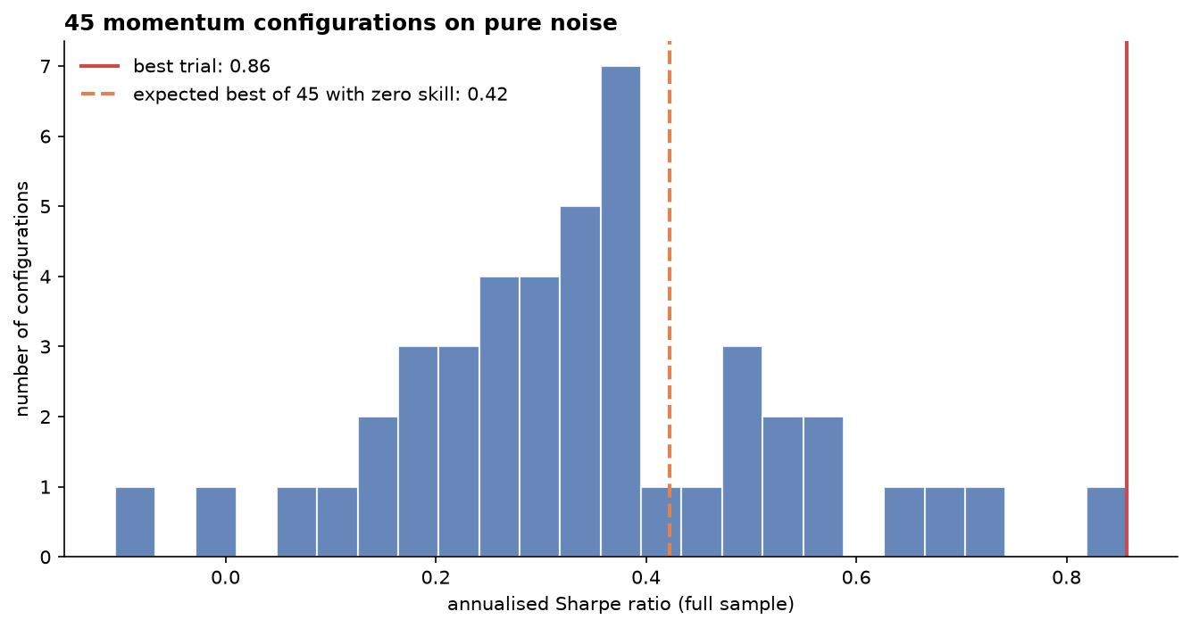
|
|
94
|
+
|
|
95
|
+
The lesson is that every in-sample defence (DSR, PBO, walk-forward) protects against
|
|
96
|
+
*selection* bias but not against a lucky *sample*. Only independent data (other markets,
|
|
97
|
+
periods, or asset classes) does that.
|
|
98
|
+
|
|
99
|
+
The two refinements cut in opposite directions. Counting all 45 near-duplicate configurations as
|
|
100
|
+
independent trials makes the Deflated Sharpe too strict; clustering them (`effective_trials`)
|
|
101
|
+
is more accurate, but it removes the margin that rejected this lucky sample. The cluster count also
|
|
102
|
+
depends on the correlation threshold: here it is 1, 2, 10 and 35 at ρ > 0.3, 0.5, 0.7 and 0.9.
|
|
103
|
+
The threshold-free eigenvalue participation ratio is about 3, which supports the 0.5 default.
|
|
104
|
+
|
|
105
|
+
## Study 2: survivorship bias
|
|
106
|
+
|
|
107
|
+
150 firms are listed over 12 years; 57 fail, after a decline, with a −50% final return.
|
|
108
|
+
Testing only on the 93 survivors:
|
|
109
|
+
|
|
110
|
+
| Strategy | Point-in-time universe | Survivors only |
|
|
111
|
+
|---|---|---|
|
|
112
|
+
| Equal-weight: annual return | 9.3% | **12.8%** |
|
|
113
|
+
| Equal-weight: Sharpe | 0.67 | 0.88 |
|
|
114
|
+
| Long-only momentum: annual return | 16.1% | 15.6% |
|
|
115
|
+
|
|
116
|
+
The bias is large for strategies that would have held the failures, and nearly absent for
|
|
117
|
+
momentum, which sells declining firms before they delist. The engine handles this correctly:
|
|
118
|
+
assets cannot be bought before listing, and delisted holdings become cash.
|
|
119
|
+
|
|
120
|
+
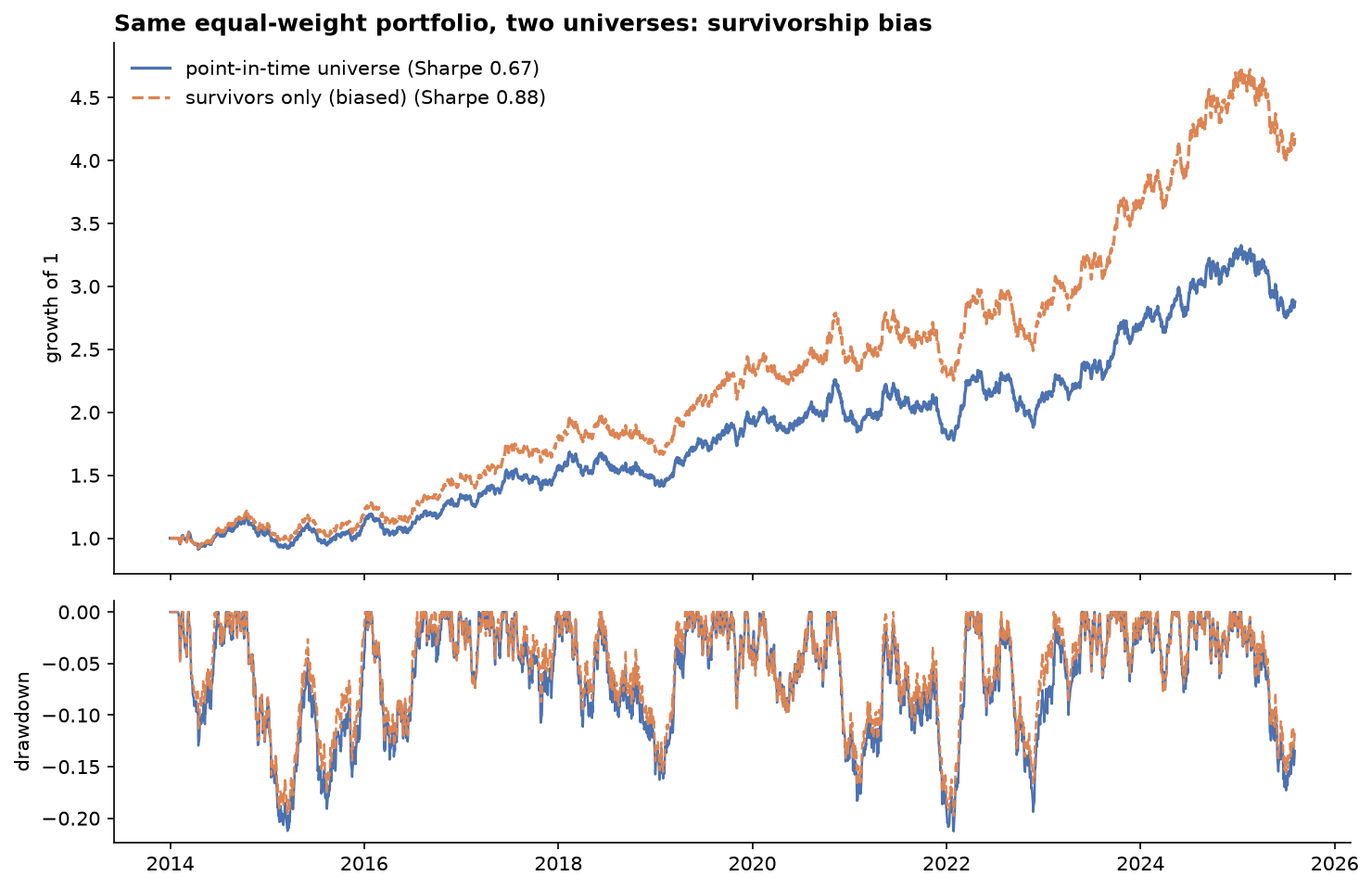
|
|
121
|
+
|
|
122
|
+
## Study 3: a genuine signal, and what costs leave of it
|
|
123
|
+
|
|
124
|
+
With a planted persistent-return effect, every check agrees the signal is real: the
|
|
125
|
+
look-ahead test passes, the Deflated Sharpe is 0.996 (1.000 with effective N = 2), and walk-forward
|
|
126
|
+
out-of-sample Sharpe, after the costs of switching configuration, is 1.01 against 1.06 in the full sample.
|
|
127
|
+
|
|
128
|
+
PBO is 0.54, no better than on noise, and that is the correct answer to a narrower question.
|
|
129
|
+
PBO asks whether picking the in-sample winner *among these configurations* beats picking one at
|
|
130
|
+
random. All 45 variants capture the same signal, so choosing among them adds nothing. A high PBO
|
|
131
|
+
says "don't trust the tuning", not "there is no edge".
|
|
132
|
+
|
|
133
|
+
Factor attribution against the market (equal-weight index) separates the edge from exposure:
|
|
134
|
+
|
|
135
|
+
| | Alpha | t-stat | Market beta | R² |
|
|
136
|
+
|---|---|---|---|---|
|
|
137
|
+
| Long-short momentum | 6.1%/yr | 3.3 | 0.01 | 0.00 |
|
|
138
|
+
| Long-only momentum | 6.8%/yr | 3.0 | 1.03 | 0.82 |
|
|
139
|
+
|
|
140
|
+
The long-only version earns 16%/yr in raw terms, but most of that is beta.
|
|
141
|
+
|
|
142
|
+
The remaining question is economic. At ~6.4× annual turnover, net Sharpe falls from 1.11
|
|
143
|
+
gross to 0.79 at 30 bps and 0.58 at 50 bps. Borrowing the short leg costs more: a 50 bps/yr
|
|
144
|
+
general-collateral fee takes Sharpe from 1.06 to 1.01, and a 300 bps/yr hard-to-borrow fee takes it to 0.80.
|
|
145
|
+
|
|
146
|
+
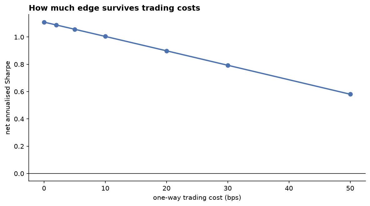
|
|
147
|
+
|
|
148
|
+
## Study 4: real data
|
|
149
|
+
|
|
150
|
+
`04_live_sector_momentum.py` runs long-short momentum across the 11 SPDR sector ETFs since
|
|
151
|
+
2000. Sector ETFs are a deliberately survivorship-free universe; late launches (XLRE, XLC)
|
|
152
|
+
enter only once listed. For single stocks, a point-in-time constituent list is required.
|
|
153
|
+
|
|
154
|
+
Over 2000 to October 2026, the result at 3 bps is a Sharpe of 0.12 (95% CI −0.23 to 0.47), and it
|
|
155
|
+
is gone by 20 bps. Regressed on the Fama-French factors plus momentum:
|
|
156
|
+
|
|
157
|
+
| | Coef | Newey-West t |
|
|
158
|
+
|---|---|---|
|
|
159
|
+
| Alpha | −0.5%/yr | −0.4 |
|
|
160
|
+
| Market | 0.02 | 2.0 |
|
|
161
|
+
| Size (SMB) | −0.02 | −1.3 |
|
|
162
|
+
| Value (HML) | −0.08 | −5.5 |
|
|
163
|
+
| **Momentum** | **0.40** | **39.6** |
|
|
164
|
+
|
|
165
|
+
R² is 0.58. Sector momentum is not a new strategy: it is a weak, diluted copy of the stock-level
|
|
166
|
+
momentum factor, which you could hold directly.
|
|
167
|
+
|
|
168
|
+
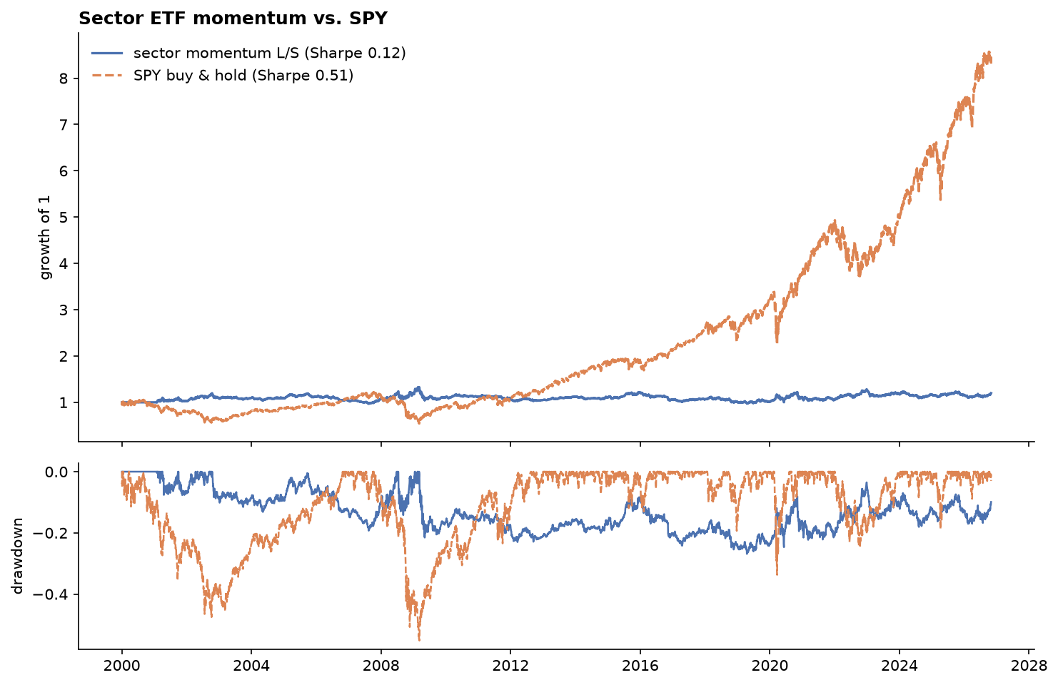
|
|
169
|
+
|
|
170
|
+
## Study 5: capacity
|
|
171
|
+
|
|
172
|
+
Flat basis-point costs ignore size. `run_backtest(..., dollar_volume=, capital=)` adds
|
|
173
|
+
square-root market impact, charging `σ_daily × √(trade / ADV)` per unit traded. On the Study 3
|
|
174
|
+
market, with a median stock trading $20m/day:
|
|
175
|
+
|
|
176
|
+
| Capital | Net Sharpe, monthly | Net Sharpe, quarterly | Cost/yr, monthly |
|
|
177
|
+
|---|---|---|---|
|
|
178
|
+
| $1m | 0.96 | 0.94 | 0.8% |
|
|
179
|
+
| $10m | 0.76 | 0.82 | 1.9% |
|
|
180
|
+
| $100m | 0.13 | 0.43 | 5.3% |
|
|
181
|
+
| $300m | −0.49 | 0.06 | 8.9% |
|
|
182
|
+
| $1bn | −1.41 | −0.52 | 16.1% |
|
|
183
|
+
|
|
184
|
+
The edge that survives 30 bps of flat costs is gone by about $150m. Rebalancing quarterly
|
|
185
|
+
gives up a little at small size but roughly doubles capacity. The square-root law is
|
|
186
|
+
calibrated for trades below about 10–20% of daily volume, so the far right of the curve
|
|
187
|
+
(where trades exceed ADV) is indicative only.
|
|
188
|
+
|
|
189
|
+
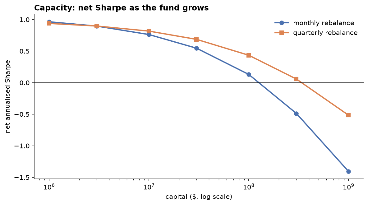
|
|
190
|
+
|
|
191
|
+
## Roadmap
|
|
192
|
+
|
|
193
|
+
- [x] **M1** Engine, strategies, look-ahead test, walk-forward, PSR/DSR, bootstrap CIs, four studies
|
|
194
|
+
- [x] **M2** Probability of Backtest Overfitting via combinatorially symmetric cross-validation
|
|
195
|
+
- [x] **M3** Effective number of trials (cluster correlated configurations) for a sharper DSR
|
|
196
|
+
- [x] **M4** Realistic costs: spread plus square-root market impact as a function of trade size and volume
|
|
197
|
+
- [x] **M5** Factor attribution: regress returns on market, size, value and momentum factors to separate alpha from beta
|
|
198
|
+
- [x] **M6** Walk-forward pays to switch configuration; borrow fees on shorts; point-in-time universe recipe
|
|
199
|
+
|
|
200
|
+
A real-data single-stock study remains out of scope: free sources such as Yahoo Finance drop
|
|
201
|
+
delisted tickers, so it needs a survivorship-free database (e.g. CRSP or Norgate) plus
|
|
202
|
+
historical index membership.
|
|
203
|
+
|
|
204
|
+
## Contributing
|
|
205
|
+
|
|
206
|
+
See [CONTRIBUTING.md](CONTRIBUTING.md) for the project's invariants, roles, workflow and
|
|
207
|
+
testing rules, and [CHANGELOG.md](CHANGELOG.md) for what changed between versions.
|
|
208
|
+
|
|
209
|
+
## References
|
|
210
|
+
|
|
211
|
+
- Bailey, D. & López de Prado, M. (2012). The Sharpe Ratio Efficient Frontier. *Journal of Risk* 15(2).
|
|
212
|
+
- Bailey, D. & López de Prado, M. (2014). The Deflated Sharpe Ratio. *Journal of Portfolio Management* 40(5).
|
|
213
|
+
- Bailey, D., Borwein, J., López de Prado, M. & Zhu, Q. (2017). The Probability of Backtest Overfitting. *Journal of Computational Finance* 20(4).
|
|
214
|
+
- Politis, D. & Romano, J. (1994). The Stationary Bootstrap. *JASA* 89(428).
|
|
215
|
+
- Jegadeesh, N. & Titman, S. (1993). Returns to Buying Winners and Selling Losers. *Journal of Finance* 48(1).
|
|
216
|
+
- López de Prado, M. & Lewis, M. (2019). Detection of False Investment Strategies Using Unsupervised Learning Methods. *Quantitative Finance* 19(9).
|
|
217
|
+
- Almgren, R., Thum, C., Hauptmann, E. & Li, H. (2005). Direct Estimation of Equity Market Impact. *Risk* 18(7).
|
|
218
|
+
- Newey, W. & West, K. (1987). A Simple, Positive Semi-Definite, Heteroskedasticity and Autocorrelation Consistent Covariance Matrix. *Econometrica* 55(3).
|
|
219
|
+
- Fama, E. & French, K. (1993). Common Risk Factors in the Returns on Stocks and Bonds. *Journal of Financial Economics* 33(1).
|
|
220
|
+
- Carhart, M. (1997). On Persistence in Mutual Fund Performance. *Journal of Finance* 52(1).
|
|
@@ -0,0 +1,12 @@
|
|
|
1
|
+
btlab/__init__.py,sha256=bPBc9PxMx_dIyjSHu9j5XiTi39yMkPlwQ8Fo685mfSU,1209
|
|
2
|
+
btlab/data.py,sha256=hJZAHdiPhQNz-P7fqRfISCPN7h-Z-GmEGHmby1OW5zw,5299
|
|
3
|
+
btlab/engine.py,sha256=Hn85qR9hlqcSyehXaouIwF1Rk6BKZ-Y9lCvjmjaACVs,7270
|
|
4
|
+
btlab/metrics.py,sha256=6OoJUko2hEfJXZdjdPsSS6mxT7RWH6hbtYDjxHdui5Y,7105
|
|
5
|
+
btlab/plotting.py,sha256=A_CJ769Evt7BYJw4-nFJ4kPydqhuS9DxQCVuDgxuJsw,4021
|
|
6
|
+
btlab/strategies.py,sha256=1hnPpKOVK4PPJLj9uRVYJM1tJssueRpLA2IuRVw_niM,2478
|
|
7
|
+
btlab/validation.py,sha256=yUqL4ONkOuXinWoMfzvHFP4C7m6FdT4_pqdH9ovrvqU,7216
|
|
8
|
+
btlab-0.3.0.dist-info/licenses/LICENSE,sha256=OAV_RTERHYKJrtHIxvr_VWUiM6k-1PKksx8ezi9wMmY,1079
|
|
9
|
+
btlab-0.3.0.dist-info/METADATA,sha256=pShPqdp1XxlOIJ2Q-8CNE01XC6TyW75Kd4fs84Pq_4g,11788
|
|
10
|
+
btlab-0.3.0.dist-info/WHEEL,sha256=mOdXR9C3wMVov7cSY8PY-XCzo3SmmWCHvGQr5csJoao,91
|
|
11
|
+
btlab-0.3.0.dist-info/top_level.txt,sha256=i3k1OKsUPFcLG3qVwtlEjSxAnAIIYcLHwQBHj6udjt4,6
|
|
12
|
+
btlab-0.3.0.dist-info/RECORD,,
|
|
@@ -0,0 +1,21 @@
|
|
|
1
|
+
MIT License
|
|
2
|
+
|
|
3
|
+
Copyright (c) 2026 Yousuf Hossain Shafeen
|
|
4
|
+
|
|
5
|
+
Permission is hereby granted, free of charge, to any person obtaining a copy
|
|
6
|
+
of this software and associated documentation files (the "Software"), to deal
|
|
7
|
+
in the Software without restriction, including without limitation the rights
|
|
8
|
+
to use, copy, modify, merge, publish, distribute, sublicense, and/or sell
|
|
9
|
+
copies of the Software, and to permit persons to whom the Software is
|
|
10
|
+
furnished to do so, subject to the following conditions:
|
|
11
|
+
|
|
12
|
+
The above copyright notice and this permission notice shall be included in all
|
|
13
|
+
copies or substantial portions of the Software.
|
|
14
|
+
|
|
15
|
+
THE SOFTWARE IS PROVIDED "AS IS", WITHOUT WARRANTY OF ANY KIND, EXPRESS OR
|
|
16
|
+
IMPLIED, INCLUDING BUT NOT LIMITED TO THE WARRANTIES OF MERCHANTABILITY,
|
|
17
|
+
FITNESS FOR A PARTICULAR PURPOSE AND NONINFRINGEMENT. IN NO EVENT SHALL THE
|
|
18
|
+
AUTHORS OR COPYRIGHT HOLDERS BE LIABLE FOR ANY CLAIM, DAMAGES OR OTHER
|
|
19
|
+
LIABILITY, WHETHER IN AN ACTION OF CONTRACT, TORT OR OTHERWISE, ARISING FROM,
|
|
20
|
+
OUT OF OR IN CONNECTION WITH THE SOFTWARE OR THE USE OR OTHER DEALINGS IN THE
|
|
21
|
+
SOFTWARE.
|
|
@@ -0,0 +1 @@
|
|
|
1
|
+
btlab
|