dolphindb 3.0.34 → 3.0.35
This diff represents the content of publicly available package versions that have been released to one of the supported registries. The information contained in this diff is provided for informational purposes only and reflects changes between package versions as they appear in their respective public registries.
- package/docs.d.ts +2 -4
- package/docs.en.json +7848 -7848
- package/docs.js +1 -12
- package/docs.js.map +1 -1
- package/docs.zh.json +413 -413
- package/package.json +1 -1
package/docs.zh.json
CHANGED
|
@@ -5552,7 +5552,7 @@
|
|
|
5552
5552
|
]
|
|
5553
5553
|
}
|
|
5554
5554
|
],
|
|
5555
|
-
"markdown": "### [createWindowJoinEngine](https://docs.dolphindb.cn/zh/funcs/c/createWindowJoinEngine.html)\n\n\n\n#### 语法\n\n`createWindowJoinEngine(name, leftTable, rightTable, outputTable, window, metrics, matchingColumn, [timeColumn], [useSystemTime=false], [garbageSize = 5000], [maxDelayedTime], [nullFill], \\[outputElapsedMicroseconds=false\\], [sortByTime=false],\\[closed\\])`\n\n#### 详情\n\n创建流数据 window join 引擎。返回一个左、右两表实时 [window join](https://docs.dolphindb.cn/zh/progr/sql/windowjoin.html) 后的表对象。\n\n该引擎与 window join 存在以下区别:\n\n* window join 仅支持聚合计算,window join 引擎支持聚合计算,也支持非聚合计算。\n* 计算指标中的列未指定表名时,window join 默认取右表列,而 window join 引擎默认取左表列。\n\n注入 window join 引擎左、右两表的数据,根据 *matchingColumn* 分组。在各分组内,左表的每条记录,都会同右表中一个时间区间(即窗口)内的数据进行连接,并根据指定的 *metrics* 计算窗口内的数据并输出。\n\n* 普通窗口(*window* 不为 0:0):\n\n 右表的计算窗口将由左表当前数据的时间戳和 *window* 确定。假设左表当前记录的时间戳为 t,*window* 为 a:b,则右表时间戳属于 \\[t+a, t+b] 的数据将与左表当前记录连接并计算输出。\n\n 触发计算的规则:\n\n * *useSystemTime*=false:\n * \\*\\*同组数据触发:\\*\\*各分组当前窗口数据的计算将由该窗口结束后的第一条属于该分组的数据触发。触发计算的数据不参与该窗口的计算。\n * \\*\\*其它分组数据触发:\\*\\*对于某个分组中未发生计算的窗口,若其窗口右边界 + *maxDelayedTime* < 右表最新收到的任意一个分组数据的时间戳,则该窗口的计算将被新收到的这条数据触发。\n * *useSystemTime*=true:各个分组收到的左表数据将触发对应分组窗口的数据计算输出。\n* 特殊窗口(*window* 为 0:0):\n\n 右表的计算窗口将由左表当前数据和其上一条数据的时间戳决定。默认情况下,该窗口左闭右开,假设左表当前记录的时间戳为 t,上一条记录的时间戳为 t0,则右表计算窗口为 \\[t0, t)。可以通过指定参数 *closed* = “right”,设置窗口为左开右闭。 触发计算的规则:\n\n * *useSystemTime*=false:各分组当前窗口数据的计算将由窗口结束后的第一条属于该分组的右表数据触发。\n * *useSystemTime*=true:各个分组收到的左表数据将触发对应分组窗口的数据计算输出。\n\n**Note:**\n\n*window*=0:0 时,若 *metrics* 中指定了非聚合的指标,其输出列必须为对应类型的 array vector。\n\n更多流数据引擎的应用场景说明可以参考 [内置流式计算引擎](https://docs.dolphindb.cn/zh/funcs/themes/streamingEngine.html)。\n\n#### 参数\n\n**name** 必选参数,表示 window join 引擎的名称,作为其在一个数据节点/计算节点上的唯一标识。可包含字母,数字和下划线,但必须以字母开头。\n\n**leftTable** 表对象。可以不包含数据,但结构必须与订阅的流数据表相同。2.00.9.3 版本开始支持 array vector 类型。\n\n**rightTable** 表对象。可以不包含数据,但结构必须与订阅的流数据表相同。\n\n**outputTable** 必选参数,为计算结果的输出表。window join 引擎会将计算结果插入该表。\n\n* 输出表各列的顺序如下:\n\n 1. 时间列。其中:\n\n * 若 *useSystemTime* = true,为 TIMESTAMP 类型;\n\n * 若 *useSystemTime* = false,数据类型与 *timeColumn* 列一致。\n\n 2. 连接列。与 *matchingColumn* 中的列以及其顺序一致,可为多列。\n\n 3. 计算结果列。可为多列。\n\n 4. 耗时列。若指定 *outputElapsedMicroseconds* = true,则需要增加一个 LONG 类型和一个 INT 类型的列,分别用于存储引擎内部每个 batch 的数据耗时(单位:微秒)和记录数。\n\n**window** 必选参数,表示滑动窗口区间的整型或 DURATION 数据对,其中左右边界都包含在内。\n\n**metrics** 以元代码的格式表示计算指标,支持输入元组。有关元代码的更多信息可参考 [元编程](https://docs.dolphindb.cn/zh/progr/objs/meta_progr.html)。\n\n* 计算指标可以是一个或多个表达式、系统内置或用户自定义函数。\n* *metrics* 内支持调用具有多个返回值的函数,且必须指定列名,例如 \\<func(price) as \\`col1\\`col2>。\n\n 若在 *metrics* 指定了 *leftTable* 和 *rightTable* 中具有相同名称的列,默认取左表的列,可以通过 \"tableName.colName\" 指定该列来自哪个表。\n\n **Note:**\n\n * *metrics* 中使用的列名大小写不敏感,不要求与输入表的列名大小写保持一致。\n * 当以下函数只计算 *rightTable* 中的数据列时,window join 引擎对它们进行了优化:sum, sum2, avg, std, var, corr, covar, wavg, wsum, beta, max, min, last, first, med, percentile。\n\n**matchingColumn** 表示连接列的字符串标量/向量/tuple,支持 Integral, Temporal 或 Literal(UUID 除外)类型。*matchingColumn* 指定规则为:\n\n1. 只有一个连接列:当左表和右表的连接列名相同时,*matchingColumn* 是一个字符串标量,否则是一个长度为 2 的 tuple,例如:左表连接列名为 sym,右表连接列名为 sym1,则 *matchingColumn* = \\[\\[\\`sym],\\[\\`sym1]]。\n\n2. 有多个连接列:当左表和右表的连接列名相同时,*matchingColumn* 是一个字符串向量,否则是一个长度为 2 的 tuple,例如:左表连接列名为 timestamp, sym,右表连接列名为 timestamp, sym1,则 *matchingColumn* = \\[\\[\\`timestamp, \\`sym], \\[\\`timestamp,\\`sym1]]。\n\n**timeColumn** 可选参数,当 *useSystemTime* = false时,指定要连接的两个表中时间列的名称。*leftTable* 和 *rightTable* 时间列名称可以不同,但数据类型需保持一致。当 *leftTable* 和 *rightTable* 时间列名称不同时,*timeColumn* 为一个长度为2的字符串向量。\n\n**useSystemTime** 可选参数,表示 *outputTable* 中第一列(时间列)为系统当前时间(*useSystemTime* = true)或左表的时间列(*useSystemTime* = false)。\n\n**garbageSize** 可选参数,是正整数,默认值是5,000(单位为行)。随着订阅的流数据不断积累进入 window join 引擎,存放在内存中的数据会越来越多,这时需要清理不再需要的历史数据。当左/右两表各个分组内的数据行数超过 *garbageSize* 值时,系统会清理本次计算不需要的历史数据。\n\n**maxDelayedTime** 可选参数,是正整数,默认值为3,单位为秒。通过设置该参数,帮助触发引擎中长时间未输出的分组数据进行计算。 即若`(某个分组中未发生计算的窗口右边界) + (maxDelayedTime) < (右表最新收到的任意一个分组数据的时间戳)`,则这条数据会触发该窗口计算输出。\n\n**Note:** 指定该参数时,必须同时指定 timeColumn,且单位需和 timeColumn 精度一致。\n\n**nullFill** 和输出表列字段等长且类型一一对应的元组,用于填充以下列中的空值:输出表中包含的左表列、右表列、右表列被聚合计算后的计算结果列。\n\n若同时有一批数据注入引擎,则引擎内部数据是分批进行计算的,每个批次的数据称为一个 batch,每个 batch 包含记录数由系统决定。\n\n**outputElapsedMicroseconds** 布尔值,表示是否输出每个 batch 中数据从注入引擎到计算输出的总耗时,以及每个 batch 包含的总记录数,默认为 false。指定参数 *outputElapsedMicroseconds* = true 后,在定义 *outputTables* 时需要在最后增加两列,详见 *outputTable* 参数说明。\n\n**sortByTime** 布尔值,表示是否按全局时间顺序输出数据。默认值为 false,表示不按全局时间输出数据,仅在组内按时间顺序输出数据。注意:当设置 sortByTime=true 时,必须保证输入的左表和右表的数据必须全局有序,且不可设置 *maxDelayedTime*。\n\n**closed** 字符串,用于确定窗口边界的开闭情况,仅当 *window*为 0:0 时有效 。可选值为 ‘left’ 或 ‘right’,默认值为 ‘left’。\n\n* closed = ‘left’: 窗口左闭右开。\n\n* closed = ‘right’: 窗口左开右闭。此时必须设置 useSystemTime=false 。\n\n#### 例子\n\n```\nshare streamTable(1:0, `time`sym`price, [TIMESTAMP, SYMBOL, DOUBLE]) as leftTable\nshare streamTable(1:0, `time`sym`val, [TIMESTAMP, SYMBOL, DOUBLE]) as rightTable\nshare table(100:0, `time`sym`factor1`factor2`factor3, [TIMESTAMP, SYMBOL, DOUBLE, DOUBLE, DOUBLE]) as output\n\nnullFill= [2012.01.01T00:00:00.000, `NONE, 0.0, 0.0, 0.0]\nwjEngine=createWindowJoinEngine(name=\"test1\", leftTable=leftTable, rightTable=rightTable, outputTable=output, window=-2:2, metrics=<[price,val,sum(val)]>, matchingColumn=`sym, timeColumn=`time, useSystemTime=false,nullFill=nullFill)\n\nsubscribeTable(tableName=\"leftTable\", actionName=\"joinLeft\", offset=0, handler=appendForJoin{wjEngine, true}, msgAsTable=true)\nsubscribeTable(tableName=\"rightTable\", actionName=\"joinRight\", offset=0, handler=appendForJoin{wjEngine, false}, msgAsTable=true)\n\nn=10\ntp1=table(take(2012.01.01T00:00:00.000+0..10, 2*n) as time, take(`A, n) join take(`B, n) as sym, take(NULL join rand(10.0, n-1),2*n) as price)\ntp1.sortBy!(`time)\nleftTable.append!(tp1)\n\ntp2=table(take(2012.01.01T00:00:00.000+0..10, 2*n) as time, take(`A, n) join take(`B, n) as sym, take(double(1..n),2*n) as val)\ntp2.sortBy!(`time)\nrightTable.append!(tp2)\n\nselect * from output where time between 2012.01.01T00:00:00.000:2012.01.01T00:00:00.001\n```\n\n| time | sym | factor1 | factor2 | factor3 |\n| ----------------------- | --- | ------- | ------- | ------- |\n| 2012.01.01T00:00:00.000 | A | 0 | 1 | 6 |\n| 2012.01.01T00:00:00.000 | A | 0 | 2 | 6 |\n| 2012.01.01T00:00:00.000 | A | 0 | 3 | 6 |\n| 2012.01.01T00:00:00.001 | A | 5.2705 | 1 | 10 |\n| 2012.01.01T00:00:00.001 | A | 5.2705 | 2 | 10 |\n| 2012.01.01T00:00:00.001 | A | 5.2705 | 3 | 10 |\n| 2012.01.01T00:00:00.001 | A | 5.2705 | 4 | 10 |\n| 2012.01.01T00:00:00.000 | B | 5.2705 | 2 | 9 |\n| 2012.01.01T00:00:00.000 | B | 5.2705 | 3 | 9 |\n| 2012.01.01T00:00:00.000 | B | 5.2705 | 4 | 9 |\n| 2012.01.01T00:00:00.001 | B | 1.0179 | 2 | 14 |\n| 2012.01.01T00:00:00.001 | B | 1.0179 | 3 | 14 |\n| 2012.01.01T00:00:00.001 | B | 1.0179 | 4 | 14 |\n| 2012.01.01T00:00:00.001 | B | 1.0179 | 5 | 14 |\n\n下例展示特殊窗口的计算:\n\n```\nshare streamTable(1:0, `time`sym`price, [TIMESTAMP, SYMBOL, DOUBLE]) as leftTable\nshare streamTable(1:0, `time`sym`val, [TIMESTAMP, SYMBOL, DOUBLE]) as rightTable\n\nv = [1, 5, 10, 15]\ntp1=table(2012.01.01T00:00:00.000+v as time, take(`A , 4) as sym, rand(10.0,4) as price)\n\nv = [1, 2, 3, 4, 5, 6, 9, 15]\ntp2=table(2012.01.01T00:00:00.000+v as time, take(`A , 8) as sym, rand(10.0,8) as val)\n\nshare table(100:0, `time`sym`price`val`sum_val, [TIMESTAMP, SYMBOL, DOUBLE, DOUBLE[], DOUBLE]) as output\nwjEngine=createWindowJoinEngine(name=\"test1\", leftTable=leftTable, rightTable=rightTable, outputTable=output, window=0:0, metrics=<[price, val, sum(val)]>, matchingColumn=`sym, timeColumn=`time, useSystemTime=false)\n\nsubscribeTable(tableName=\"leftTable\", actionName=\"joinLeft\", offset=0, handler=appendForJoin{wjEngine, true}, msgAsTable=true)\nsubscribeTable(tableName=\"rightTable\", actionName=\"joinRight\", offset=0, handler=appendForJoin{wjEngine, false}, msgAsTable=true)\n\nleftTable.append!(tp1)\nrightTable.append!(tp2)\n```\n\n| time | sym | price | val | sum\\_val |\n| ----------------------- | --- | ------ | --------------------------------- | -------- |\n| 2012.01.01T00:00:00.001 | A | 8.8252 | \\[] | |\n| 2012.01.01T00:00:00.005 | A | 7.1195 | \\[7.495792,9.417891,1.419681,...] | 21.3741 |\n| 2012.01.01T00:00:00.010 | A | 5.2217 | \\[4.840462,8.086567,3.495306] | 16.4223 |\n| 2012.01.01T00:00:00.015 | A | 9.2517 | \\[] | |\n\n当 window=0:0 时,默认情况下,该窗口左闭右开。下例中指定参数 *closed* = \"right\",将窗口设置为左开右闭。\n\n```\nunsubscribeTable(tableName=\"leftTable\", actionName=\"joinLeft\")\nunsubscribeTable(tableName=\"rightTable\", actionName=\"joinRight\")\nundef(`leftTable,SHARED)\nundef(`rightTable,SHARED)\ndropAggregator(name=\"test1\")\n\nshare streamTable(1:0, `time`sym`price, [TIMESTAMP, SYMBOL, DOUBLE]) as leftTable\nshare streamTable(1:0, `time`sym`val, [TIMESTAMP, SYMBOL, DOUBLE]) as rightTable\n\nv1 = [1, 5, 10, 15]\ntp1=table(2012.01.01T00:00:00.000+v1 as time, take(`A, 4) as sym, rand(10.0,4) as price)\n\nv2 = [1, 2, 3, 4, 5, 6, 9, 15]\ntp2=table(2012.01.01T00:00:00.000+v2 as time, take(`A, 8) as sym, rand(10.0,8) as val)\n\nshare table(100:0, `time`sym`price`val`sum_val, [TIMESTAMP, SYMBOL, DOUBLE, DOUBLE[], DOUBLE]) as output\nwjEngine=createWindowJoinEngine(name=\"test1\", leftTable=leftTable, rightTable=rightTable, outputTable=output, window=0:0, metrics=<[price, val, sum(val)]>, matchingColumn=\"sym\", timeColumn=\"time\", useSystemTime=false, closed=\"right\")\n\nsubscribeTable(tableName=\"leftTable\", actionName=\"joinLeft\", offset=0, handler=appendForJoin{wjEngine, true}, msgAsTable=true)\nsubscribeTable(tableName=\"rightTable\", actionName=\"joinRight\", offset=0, handler=appendForJoin{wjEngine, false}, msgAsTable=true)\n\nleftTable.append!(tp1)\nrightTable.append!(tp2)\nsleep(100)\nselect * from output\n```\n\n返回:\n\n```\ntime\t sym\tprice\tval\t sum_val\n2012.01.01T00:00:00.001\tA\t9.7366\t[7.8310]\t 7.831\n2012.01.01T00:00:00.005\tA\t2.6537\t[1.8564,4.6238,8.2536,3.1028] 17.8368\n2012.01.01T00:00:00.010\tA\t3.9586\t[0.8413,8.0684]\t 8.9098\n```\n\n下例展示指定 *sortByTime* = true 时,引擎将按时间顺序输出数据。\n\n```\n//清理引擎及变量\nunsubscribeTable(tableName=\"leftTable\", actionName=\"joinLeft\")\nunsubscribeTable(tableName=\"rightTable\", actionName=\"joinRight\")\nundef(`leftTable,SHARED)\nundef(`rightTable,SHARED)\ndropAggregator(name=\"test1\")\n\n//定义引擎\nshare streamTable(1:0, `time`sym`price, [TIMESTAMP, SYMBOL, DOUBLE]) as leftTable\nshare streamTable(1:0, `time`sym`val, [TIMESTAMP, SYMBOL, DOUBLE]) as rightTable\nshare table(100:0, `time`sym`factor1`factor2`factor3, [TIMESTAMP, SYMBOL, DOUBLE, DOUBLE, DOUBLE]) as output\nnullFill= [2012.01.01T00:00:00.000, `NONE, 0.0, 0.0, 0.0]\nwjEngine=createWindowJoinEngine(name=\"test1\", leftTable=leftTable, rightTable=rightTable, outputTable=output, window=-2:2, metrics=<[price,val,sum(val)]>, matchingColumn=`sym, timeColumn=`time, useSystemTime=false,nullFill=nullFill, sortByTime=true)\n\n//定义数据\nsubscribeTable(tableName=\"leftTable\", actionName=\"joinLeft\", offset=0, handler=appendForJoin{wjEngine, true}, msgAsTable=true)\nsubscribeTable(tableName=\"rightTable\", actionName=\"joinRight\", offset=0, handler=appendForJoin{wjEngine, false}, msgAsTable=true)\n\nn=10\ntp1=table(take(2012.01.01T00:00:00.000+0..10, 2*n) as time, take(`A, n) join take(`B, n) as sym, take(NULL join rand(10.0, n-1),2*n) as price)\ntp1.sortBy!(`time)\nleftTable.append!(tp1)\n\ntp2=table(take(2012.01.01T00:00:00.000+0..10, 2*n) as time, take(`A, n) join take(`B, n) as sym, take(double(1..n),2*n) as val)\ntp2.sortBy!(`time)\nrightTable.append!(tp2)\n\nsleep(100)\nselect * from output where time between 2012.01.01T00:00:00.000:2012.01.01T00:00:00.001\n```\n\n| time | sym | factor1 | factor2 | factor3 |\n| ----------------------- | --- | ------- | ------- | ------- |\n| 2012.01.01T00:00:00.000 | A | 0 | 1 | 6 |\n| 2012.01.01T00:00:00.000 | A | 0 | 2 | 6 |\n| 2012.01.01T00:00:00.000 | A | 0 | 3 | 6 |\n| 2012.01.01T00:00:00.000 | B | 3.9389 | 2 | 9 |\n| 2012.01.01T00:00:00.000 | B | 3.9389 | 3 | 9 |\n| 2012.01.01T00:00:00.000 | B | 3.9389 | 4 | 9 |\n| 2012.01.01T00:00:00.001 | A | 3.9389 | 1 | 10 |\n| 2012.01.01T00:00:00.001 | A | 3.9389 | 2 | 10 |\n| 2012.01.01T00:00:00.001 | A | 3.9389 | 3 | 10 |\n| 2012.01.01T00:00:00.001 | A | 3.9389 | 4 | 10 |\n| 2012.01.01T00:00:00.001 | B | 4.9875 | 2 | 14 |\n| 2012.01.01T00:00:00.001 | B | 4.9875 | 3 | 14 |\n| 2012.01.01T00:00:00.001 | B | 4.9875 | 4 | 14 |\n| 2012.01.01T00:00:00.001 | B | 4.9875 | 5 | 14 |\n"
|
|
5555
|
+
"markdown": "### [createWindowJoinEngine](https://docs.dolphindb.cn/zh/funcs/c/createWindowJoinEngine.html)\n\n\n\n#### 语法\n\n`createWindowJoinEngine(name, leftTable, rightTable, outputTable, window, metrics, matchingColumn, [timeColumn], [useSystemTime=false], [garbageSize = 5000], [maxDelayedTime], [nullFill], \\[outputElapsedMicroseconds=false\\], [sortByTime=false],\\[closed\\])`\n\n#### 详情\n\n创建流数据 window join 引擎。返回一个左、右两表实时 [window join](https://docs.dolphindb.cn/zh/progr/sql/windowjoin.html) 后的表对象。\n\n该引擎与 window join 存在以下区别:\n\n* window join 仅支持聚合计算,window join 引擎支持聚合计算,也支持非聚合计算。\n* 计算指标中的列未指定表名时,window join 默认取右表列,而 window join 引擎默认取左表列。\n\n注入 window join 引擎左、右两表的数据,根据 *matchingColumn* 分组。在各分组内,左表的每条记录,都会同右表中一个时间区间(即窗口)内的数据进行连接,并根据指定的 *metrics* 计算窗口内的数据并输出。\n\n* 普通窗口(*window* 不为 0:0):\n\n 右表的计算窗口将由左表当前数据的时间戳和 *window* 确定。假设左表当前记录的时间戳为 t,*window* 为 a:b,则右表时间戳属于 \\[t+a, t+b] 的数据将与左表当前记录连接并计算输出。\n\n 触发计算的规则:\n\n * *useSystemTime*=false:\n * \\*\\*同组数据触发:\\*\\*各分组当前窗口数据的计算将由该窗口结束后的第一条属于该分组的数据触发。触发计算的数据不参与该窗口的计算。\n * \\*\\*其它分组数据触发:\\*\\*对于某个分组中未发生计算的窗口,若其窗口右边界 + *maxDelayedTime* < 右表最新收到的任意一个分组数据的时间戳,则该窗口的计算将被新收到的这条数据触发。\n * *useSystemTime*=true:当系统时间到达各分组未发生计算的窗口的右边界时,触发该窗口的计算。\n* 特殊窗口(*window* 为 0:0):\n\n 右表的计算窗口将由左表当前数据和其上一条数据的时间戳决定。默认情况下,该窗口左闭右开,假设左表当前记录的时间戳为 t,上一条记录的时间戳为 t0,则右表计算窗口为 \\[t0, t)。可以通过指定参数 *closed* = “right”,设置窗口为左开右闭。 触发计算的规则:\n\n * *useSystemTime*=false:各分组当前窗口数据的计算将由窗口结束后的第一条属于该分组的右表数据触发。\n * *useSystemTime*=true:各个分组收到的左表数据将触发对应分组窗口的数据计算输出。\n\n**Note:**\n\n*window*=0:0 时,若 *metrics* 中指定了非聚合的指标,其输出列必须为对应类型的 array vector。\n\n更多流数据引擎的应用场景说明可以参考 [内置流式计算引擎](https://docs.dolphindb.cn/zh/funcs/themes/streamingEngine.html)。\n\n#### 参数\n\n**name** 必选参数,表示 window join 引擎的名称,作为其在一个数据节点/计算节点上的唯一标识。可包含字母,数字和下划线,但必须以字母开头。\n\n**leftTable** 表对象。可以不包含数据,但结构必须与订阅的流数据表相同。2.00.9.3 版本开始支持 array vector 类型。\n\n**rightTable** 表对象。可以不包含数据,但结构必须与订阅的流数据表相同。\n\n**outputTable** 必选参数,为计算结果的输出表。window join 引擎会将计算结果插入该表。\n\n* 输出表各列的顺序如下:\n\n 1. 时间列。其中:\n\n * 若 *useSystemTime* = true,为 TIMESTAMP 类型;\n\n * 若 *useSystemTime* = false,数据类型与 *timeColumn* 列一致。\n\n 2. 连接列。与 *matchingColumn* 中的列以及其顺序一致,可为多列。\n\n 3. 计算结果列。可为多列。\n\n 4. 耗时列。若指定 *outputElapsedMicroseconds* = true,则需要增加一个 LONG 类型和一个 INT 类型的列,分别用于存储引擎内部每个 batch 的数据耗时(单位:微秒)和记录数。\n\n**window** 必选参数,表示滑动窗口区间的整型或 DURATION 数据对,其中左右边界都包含在内。\n\n**metrics** 以元代码的格式表示计算指标,支持输入元组。有关元代码的更多信息可参考 [元编程](https://docs.dolphindb.cn/zh/progr/objs/meta_progr.html)。\n\n* 计算指标可以是一个或多个表达式、系统内置或用户自定义函数。\n* *metrics* 内支持调用具有多个返回值的函数,且必须指定列名,例如 \\<func(price) as \\`col1\\`col2>。\n\n 若在 *metrics* 指定了 *leftTable* 和 *rightTable* 中具有相同名称的列,默认取左表的列,可以通过 \"tableName.colName\" 指定该列来自哪个表。\n\n **Note:**\n\n * *metrics* 中使用的列名大小写不敏感,不要求与输入表的列名大小写保持一致。\n * 当以下函数只计算 *rightTable* 中的数据列时,window join 引擎对它们进行了优化:sum, sum2, avg, std, var, corr, covar, wavg, wsum, beta, max, min, last, first, med, percentile。\n\n**matchingColumn** 表示连接列的字符串标量/向量/tuple,支持 Integral, Temporal 或 Literal(UUID 除外)类型。*matchingColumn* 指定规则为:\n\n1. 只有一个连接列:当左表和右表的连接列名相同时,*matchingColumn* 是一个字符串标量,否则是一个长度为 2 的 tuple,例如:左表连接列名为 sym,右表连接列名为 sym1,则 *matchingColumn* = \\[\\[\\`sym],\\[\\`sym1]]。\n\n2. 有多个连接列:当左表和右表的连接列名相同时,*matchingColumn* 是一个字符串向量,否则是一个长度为 2 的 tuple,例如:左表连接列名为 timestamp, sym,右表连接列名为 timestamp, sym1,则 *matchingColumn* = \\[\\[\\`timestamp, \\`sym], \\[\\`timestamp,\\`sym1]]。\n\n**timeColumn** 可选参数,当 *useSystemTime* = false时,指定要连接的两个表中时间列的名称。*leftTable* 和 *rightTable* 时间列名称可以不同,但数据类型需保持一致。当 *leftTable* 和 *rightTable* 时间列名称不同时,*timeColumn* 为一个长度为2的字符串向量。\n\n**useSystemTime** 可选参数,表示 *outputTable* 中第一列(时间列)为系统当前时间(*useSystemTime* = true)或左表的时间列(*useSystemTime* = false)。\n\n**garbageSize** 可选参数,是正整数,默认值是5,000(单位为行)。随着订阅的流数据不断积累进入 window join 引擎,存放在内存中的数据会越来越多,这时需要清理不再需要的历史数据。当左/右两表各个分组内的数据行数超过 *garbageSize* 值时,系统会清理本次计算不需要的历史数据。\n\n**maxDelayedTime** 可选参数,是正整数,默认值为3,单位为秒。通过设置该参数,帮助触发引擎中长时间未输出的分组数据进行计算。 即若`(某个分组中未发生计算的窗口右边界) + (maxDelayedTime) < (右表最新收到的任意一个分组数据的时间戳)`,则这条数据会触发该窗口计算输出。\n\n**Note:** 指定该参数时,必须同时指定 timeColumn,且单位需和 timeColumn 精度一致。\n\n**nullFill** 和输出表列字段等长且类型一一对应的元组,用于填充以下列中的空值:输出表中包含的左表列、右表列、右表列被聚合计算后的计算结果列。\n\n若同时有一批数据注入引擎,则引擎内部数据是分批进行计算的,每个批次的数据称为一个 batch,每个 batch 包含记录数由系统决定。\n\n**outputElapsedMicroseconds** 布尔值,表示是否输出每个 batch 中数据从注入引擎到计算输出的总耗时,以及每个 batch 包含的总记录数,默认为 false。指定参数 *outputElapsedMicroseconds* = true 后,在定义 *outputTables* 时需要在最后增加两列,详见 *outputTable* 参数说明。\n\n**sortByTime** 布尔值,表示是否按全局时间顺序输出数据。默认值为 false,表示不按全局时间输出数据,仅在组内按时间顺序输出数据。注意:当设置 sortByTime=true 时,必须保证输入的左表和右表的数据必须全局有序,且不可设置 *maxDelayedTime*。\n\n**closed** 字符串,用于确定窗口边界的开闭情况,仅当 *window*为 0:0 时有效 。可选值为 ‘left’ 或 ‘right’,默认值为 ‘left’。\n\n* closed = ‘left’: 窗口左闭右开。\n\n* closed = ‘right’: 窗口左开右闭。此时必须设置 useSystemTime=false 。\n\n#### 例子\n\n```\nshare streamTable(1:0, `time`sym`price, [TIMESTAMP, SYMBOL, DOUBLE]) as leftTable\nshare streamTable(1:0, `time`sym`val, [TIMESTAMP, SYMBOL, DOUBLE]) as rightTable\nshare table(100:0, `time`sym`factor1`factor2`factor3, [TIMESTAMP, SYMBOL, DOUBLE, DOUBLE, DOUBLE]) as output\n\nnullFill= [2012.01.01T00:00:00.000, `NONE, 0.0, 0.0, 0.0]\nwjEngine=createWindowJoinEngine(name=\"test1\", leftTable=leftTable, rightTable=rightTable, outputTable=output, window=-2:2, metrics=<[price,val,sum(val)]>, matchingColumn=`sym, timeColumn=`time, useSystemTime=false,nullFill=nullFill)\n\nsubscribeTable(tableName=\"leftTable\", actionName=\"joinLeft\", offset=0, handler=appendForJoin{wjEngine, true}, msgAsTable=true)\nsubscribeTable(tableName=\"rightTable\", actionName=\"joinRight\", offset=0, handler=appendForJoin{wjEngine, false}, msgAsTable=true)\n\nn=10\ntp1=table(take(2012.01.01T00:00:00.000+0..10, 2*n) as time, take(`A, n) join take(`B, n) as sym, take(NULL join rand(10.0, n-1),2*n) as price)\ntp1.sortBy!(`time)\nleftTable.append!(tp1)\n\ntp2=table(take(2012.01.01T00:00:00.000+0..10, 2*n) as time, take(`A, n) join take(`B, n) as sym, take(double(1..n),2*n) as val)\ntp2.sortBy!(`time)\nrightTable.append!(tp2)\n\nselect * from output where time between 2012.01.01T00:00:00.000:2012.01.01T00:00:00.001\n```\n\n| time | sym | factor1 | factor2 | factor3 |\n| ----------------------- | --- | ------- | ------- | ------- |\n| 2012.01.01T00:00:00.000 | A | 0 | 1 | 6 |\n| 2012.01.01T00:00:00.000 | A | 0 | 2 | 6 |\n| 2012.01.01T00:00:00.000 | A | 0 | 3 | 6 |\n| 2012.01.01T00:00:00.001 | A | 5.2705 | 1 | 10 |\n| 2012.01.01T00:00:00.001 | A | 5.2705 | 2 | 10 |\n| 2012.01.01T00:00:00.001 | A | 5.2705 | 3 | 10 |\n| 2012.01.01T00:00:00.001 | A | 5.2705 | 4 | 10 |\n| 2012.01.01T00:00:00.000 | B | 5.2705 | 2 | 9 |\n| 2012.01.01T00:00:00.000 | B | 5.2705 | 3 | 9 |\n| 2012.01.01T00:00:00.000 | B | 5.2705 | 4 | 9 |\n| 2012.01.01T00:00:00.001 | B | 1.0179 | 2 | 14 |\n| 2012.01.01T00:00:00.001 | B | 1.0179 | 3 | 14 |\n| 2012.01.01T00:00:00.001 | B | 1.0179 | 4 | 14 |\n| 2012.01.01T00:00:00.001 | B | 1.0179 | 5 | 14 |\n\n下例展示特殊窗口的计算:\n\n```\nshare streamTable(1:0, `time`sym`price, [TIMESTAMP, SYMBOL, DOUBLE]) as leftTable\nshare streamTable(1:0, `time`sym`val, [TIMESTAMP, SYMBOL, DOUBLE]) as rightTable\n\nv = [1, 5, 10, 15]\ntp1=table(2012.01.01T00:00:00.000+v as time, take(`A , 4) as sym, rand(10.0,4) as price)\n\nv = [1, 2, 3, 4, 5, 6, 9, 15]\ntp2=table(2012.01.01T00:00:00.000+v as time, take(`A , 8) as sym, rand(10.0,8) as val)\n\nshare table(100:0, `time`sym`price`val`sum_val, [TIMESTAMP, SYMBOL, DOUBLE, DOUBLE[], DOUBLE]) as output\nwjEngine=createWindowJoinEngine(name=\"test1\", leftTable=leftTable, rightTable=rightTable, outputTable=output, window=0:0, metrics=<[price, val, sum(val)]>, matchingColumn=`sym, timeColumn=`time, useSystemTime=false)\n\nsubscribeTable(tableName=\"leftTable\", actionName=\"joinLeft\", offset=0, handler=appendForJoin{wjEngine, true}, msgAsTable=true)\nsubscribeTable(tableName=\"rightTable\", actionName=\"joinRight\", offset=0, handler=appendForJoin{wjEngine, false}, msgAsTable=true)\n\nleftTable.append!(tp1)\nrightTable.append!(tp2)\n```\n\n| time | sym | price | val | sum\\_val |\n| ----------------------- | --- | ------ | --------------------------------- | -------- |\n| 2012.01.01T00:00:00.001 | A | 8.8252 | \\[] | |\n| 2012.01.01T00:00:00.005 | A | 7.1195 | \\[7.495792,9.417891,1.419681,...] | 21.3741 |\n| 2012.01.01T00:00:00.010 | A | 5.2217 | \\[4.840462,8.086567,3.495306] | 16.4223 |\n| 2012.01.01T00:00:00.015 | A | 9.2517 | \\[] | |\n\n当 window=0:0 时,默认情况下,该窗口左闭右开。下例中指定参数 *closed* = \"right\",将窗口设置为左开右闭。\n\n```\nunsubscribeTable(tableName=\"leftTable\", actionName=\"joinLeft\")\nunsubscribeTable(tableName=\"rightTable\", actionName=\"joinRight\")\nundef(`leftTable,SHARED)\nundef(`rightTable,SHARED)\ndropAggregator(name=\"test1\")\n\nshare streamTable(1:0, `time`sym`price, [TIMESTAMP, SYMBOL, DOUBLE]) as leftTable\nshare streamTable(1:0, `time`sym`val, [TIMESTAMP, SYMBOL, DOUBLE]) as rightTable\n\nv1 = [1, 5, 10, 15]\ntp1=table(2012.01.01T00:00:00.000+v1 as time, take(`A, 4) as sym, rand(10.0,4) as price)\n\nv2 = [1, 2, 3, 4, 5, 6, 9, 15]\ntp2=table(2012.01.01T00:00:00.000+v2 as time, take(`A, 8) as sym, rand(10.0,8) as val)\n\nshare table(100:0, `time`sym`price`val`sum_val, [TIMESTAMP, SYMBOL, DOUBLE, DOUBLE[], DOUBLE]) as output\nwjEngine=createWindowJoinEngine(name=\"test1\", leftTable=leftTable, rightTable=rightTable, outputTable=output, window=0:0, metrics=<[price, val, sum(val)]>, matchingColumn=\"sym\", timeColumn=\"time\", useSystemTime=false, closed=\"right\")\n\nsubscribeTable(tableName=\"leftTable\", actionName=\"joinLeft\", offset=0, handler=appendForJoin{wjEngine, true}, msgAsTable=true)\nsubscribeTable(tableName=\"rightTable\", actionName=\"joinRight\", offset=0, handler=appendForJoin{wjEngine, false}, msgAsTable=true)\n\nleftTable.append!(tp1)\nrightTable.append!(tp2)\nsleep(100)\nselect * from output\n```\n\n返回:\n\n```\ntime\t sym\tprice\tval\t sum_val\n2012.01.01T00:00:00.001\tA\t9.7366\t[7.8310]\t 7.831\n2012.01.01T00:00:00.005\tA\t2.6537\t[1.8564,4.6238,8.2536,3.1028] 17.8368\n2012.01.01T00:00:00.010\tA\t3.9586\t[0.8413,8.0684]\t 8.9098\n```\n\n下例展示指定 *sortByTime* = true 时,引擎将按时间顺序输出数据。\n\n```\n//清理引擎及变量\nunsubscribeTable(tableName=\"leftTable\", actionName=\"joinLeft\")\nunsubscribeTable(tableName=\"rightTable\", actionName=\"joinRight\")\nundef(`leftTable,SHARED)\nundef(`rightTable,SHARED)\ndropAggregator(name=\"test1\")\n\n//定义引擎\nshare streamTable(1:0, `time`sym`price, [TIMESTAMP, SYMBOL, DOUBLE]) as leftTable\nshare streamTable(1:0, `time`sym`val, [TIMESTAMP, SYMBOL, DOUBLE]) as rightTable\nshare table(100:0, `time`sym`factor1`factor2`factor3, [TIMESTAMP, SYMBOL, DOUBLE, DOUBLE, DOUBLE]) as output\nnullFill= [2012.01.01T00:00:00.000, `NONE, 0.0, 0.0, 0.0]\nwjEngine=createWindowJoinEngine(name=\"test1\", leftTable=leftTable, rightTable=rightTable, outputTable=output, window=-2:2, metrics=<[price,val,sum(val)]>, matchingColumn=`sym, timeColumn=`time, useSystemTime=false,nullFill=nullFill, sortByTime=true)\n\n//定义数据\nsubscribeTable(tableName=\"leftTable\", actionName=\"joinLeft\", offset=0, handler=appendForJoin{wjEngine, true}, msgAsTable=true)\nsubscribeTable(tableName=\"rightTable\", actionName=\"joinRight\", offset=0, handler=appendForJoin{wjEngine, false}, msgAsTable=true)\n\nn=10\ntp1=table(take(2012.01.01T00:00:00.000+0..10, 2*n) as time, take(`A, n) join take(`B, n) as sym, take(NULL join rand(10.0, n-1),2*n) as price)\ntp1.sortBy!(`time)\nleftTable.append!(tp1)\n\ntp2=table(take(2012.01.01T00:00:00.000+0..10, 2*n) as time, take(`A, n) join take(`B, n) as sym, take(double(1..n),2*n) as val)\ntp2.sortBy!(`time)\nrightTable.append!(tp2)\n\nsleep(100)\nselect * from output where time between 2012.01.01T00:00:00.000:2012.01.01T00:00:00.001\n```\n\n| time | sym | factor1 | factor2 | factor3 |\n| ----------------------- | --- | ------- | ------- | ------- |\n| 2012.01.01T00:00:00.000 | A | 0 | 1 | 6 |\n| 2012.01.01T00:00:00.000 | A | 0 | 2 | 6 |\n| 2012.01.01T00:00:00.000 | A | 0 | 3 | 6 |\n| 2012.01.01T00:00:00.000 | B | 3.9389 | 2 | 9 |\n| 2012.01.01T00:00:00.000 | B | 3.9389 | 3 | 9 |\n| 2012.01.01T00:00:00.000 | B | 3.9389 | 4 | 9 |\n| 2012.01.01T00:00:00.001 | A | 3.9389 | 1 | 10 |\n| 2012.01.01T00:00:00.001 | A | 3.9389 | 2 | 10 |\n| 2012.01.01T00:00:00.001 | A | 3.9389 | 3 | 10 |\n| 2012.01.01T00:00:00.001 | A | 3.9389 | 4 | 10 |\n| 2012.01.01T00:00:00.001 | B | 4.9875 | 2 | 14 |\n| 2012.01.01T00:00:00.001 | B | 4.9875 | 3 | 14 |\n| 2012.01.01T00:00:00.001 | B | 4.9875 | 4 | 14 |\n| 2012.01.01T00:00:00.001 | B | 4.9875 | 5 | 14 |\n"
|
|
5556
5556
|
},
|
|
5557
5557
|
"crossStat": {
|
|
5558
5558
|
"href": "https://docs.dolphindb.cn/zh/funcs/c/crossStat.html",
|
|
@@ -9697,7 +9697,7 @@
|
|
|
9697
9697
|
]
|
|
9698
9698
|
}
|
|
9699
9699
|
],
|
|
9700
|
-
"markdown": "### [format](https://docs.dolphindb.cn/zh/funcs/f/format.html)\n\n\n\n#### 语法\n\n`format(X, format)`\n\n#### 参数\n\n**X** 可以是标量或向量。\n\n**format** 是表示 *X* 格式的字符串。\n\n#### 详情\n\n把指定格式应用到给定对象。返回结果是字符串标量或向量。\n\n根据输入对象的数据类型,`format` 函数调用 [decimalFormat](https://docs.dolphindb.cn/zh/funcs/d/decimalFormat.html) 或 [temporalFormat](https://docs.dolphindb.cn/zh/funcs/t/temporalFormat.html)。\n\n
|
|
9700
|
+
"markdown": "### [format](https://docs.dolphindb.cn/zh/funcs/f/format.html)\n\n\n\n#### 语法\n\n`format(X, format)`\n\n#### 参数\n\n**X** 可以是标量或向量。\n\n**format** 是表示 *X* 格式的字符串。\n\n#### 详情\n\n把指定格式应用到给定对象。返回结果是字符串标量或向量。\n\n根据输入对象的数据类型,`format` 函数调用 [decimalFormat](https://docs.dolphindb.cn/zh/funcs/d/decimalFormat.html) 或 [temporalFormat](https://docs.dolphindb.cn/zh/funcs/t/temporalFormat.html)。\n\n有关从数字向指定格式字符串的转换,参考(表中的备注列,请参考 [decimalFormat](https://docs.dolphindb.cn/zh/funcs/d/decimalFormat.html)):\n\n| 标志 | 含义 | 备注 |\n| -- | ---------- | --- |\n| 0 | 强制数字位数 | 备注1 |\n| # | 可选数字位数 | 备注2 |\n| . | 小数点 | |\n| % | 百分号 | 备注3 |\n| E | 科学计数法的符号 | 备注4 |\n| , | 分隔符 | 备注5 |\n| ; | 表示正数和负数的符号 | 备注6 |\n\n有关 DolphinDB 时序对象的格式,参考:\n\n| 格式 | 含义 | 范围 |\n| --------- | -------- | ------------------------------------------- |\n| yyyy | 年份(4个数字) | 1000-9999 |\n| yy | 年份(2个数字 | 00-99. (00-39: 2000-2039; 40-99: 1940-1999) |\n| MM | 月份 | 1-12 |\n| MMM | 月份 | JAN, FEB, ... DEC (不区分大小写) |\n| dd | 日期 | 1-31 |\n| HH | 时(24小时制) | 0-23 |\n| hh | 时(12小时制) | 0-11 |\n| mm | 分钟 | 0-59 |\n| ss | 秒 | 0-59 |\n| aa | 上午/下午 | AM, PM. (不区分大小写) |\n| SSS | 毫秒 | 0-999 |\n| nnnnnn | 微秒 | 0-999999 |\n| nnnnnnnnn | 纳秒 | 0-999999999 |\n\n#### 例子\n\n```\nt = table(1..100 as id, (1..100 + 2018.01.01) as date, rand(100.0, 100) as price, rand(10000, 100) as qty);\nt;\n```\n\n| id | date | price | qty |\n| --- | ---------- | --------- | ---- |\n| 1 | 2018.01.02 | 70.832104 | 1719 |\n| 2 | 2018.01.03 | 12.22557 | 6229 |\n| 3 | 2018.01.04 | 8.695886 | 1656 |\n| 4 | 2018.01.05 | 24.324535 | 2860 |\n| 5 | 2018.01.06 | 0.443173 | 6874 |\n| 6 | 2018.01.07 | 90.302176 | 3277 |\n| 7 | 2018.01.08 | 78.556843 | 3424 |\n| 8 | 2018.01.09 | 45.836447 | 8636 |\n| 9 | 2018.01.10 | 57.416425 | 707 |\n| 10 | 2018.01.11 | 98.879764 | 2267 |\n| ... | | | |\n\n```\nselect id, date.format(\"MM/dd/yyyy\") as date, price.format(\"00.00\") as price, qty.format(\"#,###\") as qty from t;\n```\n\n| id | date | price | qty |\n| --- | ---------- | ----- | ----- |\n| 1 | 01/02/2018 | 70.83 | 1,719 |\n| 2 | 01/03/2018 | 12.23 | 6,229 |\n| 3 | 01/04/2018 | 08.70 | 1,656 |\n| 4 | 01/05/2018 | 24.32 | 2,860 |\n| 5 | 01/06/2018 | 00.44 | 6,874 |\n| 6 | 01/07/2018 | 90.30 | 3,277 |\n| 7 | 01/08/2018 | 78.56 | 3,424 |\n| 8 | 01/09/2018 | 45.84 | 8,636 |\n| 9 | 01/10/2018 | 57.42 | 707 |\n| 10 | 01/11/2018 | 98.88 | 2,267 |\n| ... | | | |\n"
|
|
9701
9701
|
},
|
|
9702
9702
|
"fromJson": {
|
|
9703
9703
|
"href": "https://docs.dolphindb.cn/zh/funcs/f/fromJson.html",
|
|
@@ -10078,46 +10078,6 @@
|
|
|
10078
10078
|
],
|
|
10079
10079
|
"markdown": "### [hourOfDay](https://docs.dolphindb.cn/zh/funcs/h/hourOfDay.html)\n\n\n\n#### 语法\n\n`hourOfDay(X)`\n\n#### 参数\n\n**X** 可以是 TIME, MINUTE, SECOND, DATETIME, TIMESTAMP, NANOTIME, NANOTIMESTAMP 类型的标量或向量。\n\n#### 详情\n\n返回 *X* 中的小时。\n\n#### 例子\n\n```\nhourOfDay(00:46:12);\n# output\n0\n\nhourOfDay([2012.06.12T12:30:00,2012.10.28T17:35:00,2013.01.06T02:36:47,2013.04.06T08:02:14]);\n# output\n[12,17,2,8]\n```\n\n相关函数:[dayOfYear](https://docs.dolphindb.cn/zh/funcs/d/dayOfYear.html), [dayOfMonth](https://docs.dolphindb.cn/zh/funcs/d/dayOfMonth.html), [quarterOfYear](https://docs.dolphindb.cn/zh/funcs/q/quarterOfYear.html), [monthOfYear](https://docs.dolphindb.cn/zh/funcs/m/monthOfYear.html), [weekOfYear](https://docs.dolphindb.cn/zh/funcs/w/weekOfYear.html), [minuteOfHour](https://docs.dolphindb.cn/zh/funcs/m/minuteOfHour.html), [secondOfMinute](https://docs.dolphindb.cn/zh/funcs/s/secondOfMinute.html), [millisecond](https://docs.dolphindb.cn/zh/funcs/m/millisecond.html), [microsecond](https://docs.dolphindb.cn/zh/funcs/m/microsecond.html), [nanosecond](https://docs.dolphindb.cn/zh/funcs/n/nanosecond.html)\n"
|
|
10080
10080
|
},
|
|
10081
|
-
"join!": {
|
|
10082
|
-
"href": "https://docs.dolphindb.cn/zh/funcs/j/join!.html",
|
|
10083
|
-
"signatures": [
|
|
10084
|
-
{
|
|
10085
|
-
"full": "join!(X, Y)",
|
|
10086
|
-
"name": "join!",
|
|
10087
|
-
"parameters": [
|
|
10088
|
-
{
|
|
10089
|
-
"full": "X",
|
|
10090
|
-
"name": "X"
|
|
10091
|
-
},
|
|
10092
|
-
{
|
|
10093
|
-
"full": "Y",
|
|
10094
|
-
"name": "Y"
|
|
10095
|
-
}
|
|
10096
|
-
]
|
|
10097
|
-
}
|
|
10098
|
-
],
|
|
10099
|
-
"markdown": "### [join!](https://docs.dolphindb.cn/zh/funcs/j/join!.html)\n\n\n\n#### 语法\n\n`join!(X, Y)`\n\n#### 参数\n\n**X** 可以是向量、元组、矩阵或表。\n\n**Y** 可以是标量、向量、元组、矩阵或表。\n\n如果 *X* 是向量或元组,*Y* 可以是标量、向量或元组。如果 *X* 是矩阵,*Y* 可以是向量或矩阵。如果 *X* 是表,*Y* 可以是向量或表。\n\n#### 详情\n\n把 *Y* 合并到 *X* 中,`join!` 函数会改变 *X* 的值。\n\n#### 例子\n\n如果 *X* 是向量,*Y* 可以是标量、向量或数据类型与 X 相同的元组。返回结果是长度更长的向量。\n\n```\nx=[1,2,3]\nx.join!(4)\nx;\n```\n\n输出返回:\\[1,2,3,4]\n\n```\nx.join!(5 6 7)\nx;\n```\n\n输出返回:\\[1,2,3,4,5,6,7]\n\n```\nx.join!((8,9))\nx;\n```\n\n输出返回:\\[1,2,3,4,5,6,7,8,9]\n\n如果 *X* 是元组,*Y* 可以是标量、向量或元组。返回结果是长度更长的元组。\n\n```\nx = (1,\"A\")\nx.join!(2)\nx;\n```\n\n返回:(1,\"A\",2)\n\n```\nx.join!([3,4,5])\nx;\n```\n\n返回:(1,\"A\",2,\\[3,4,5])\n\n如果配置项 appendTupleAsAWhole 设置为 true,运行以下脚本:\n\n```\nx.join!((\"B\",\"C\")) // 配置参数 appendTupleAsAWhole=true 时\nx;\n```\n\n返回:(1,\"A\",2,\\[3,4,5],(\"B\",\"C\"))\n\n如果配置项 appendTupleAsAWhole 设置为 false,运行以上脚本后,返回:(1,\"A\",2,\\[3,4,5],\"B\",\"C\")\n\n如果 *X* 是矩阵,*Y* 可以是向量或者是与 *X* 行数相同的矩阵。返回结果是与 *X* 行数相同的矩阵。\n\n```\nx=1..6$2:3\njoin!(x, [7,8])\nx;\n```\n\n输出返回:\n\n| #0 | #1 | #2 | #3 |\n| -- | -- | -- | -- |\n| 1 | 3 | 5 | 7 |\n| 2 | 4 | 6 | 8 |\n\n```\nx.join!(9..12$2:2)\nx;\n```\n\n输出返回:\n\n| #0 | #1 | #2 | #3 | #4 | #5 |\n| -- | -- | -- | -- | -- | -- |\n| 1 | 3 | 5 | 7 | 9 | 11 |\n| 2 | 4 | 6 | 8 | 10 | 12 |\n\n如果 *X* 是表,*Y* 必须是和 *X* 行数相同的表或向量。返回结果是与 *X* 行数相同的表。\n\n```\na=table(1..3 as x, 4.5 6.7 8.5 as y);\na;\n```\n\n输出返回:\n\n| x | y |\n| - | --- |\n| 1 | 4.5 |\n| 2 | 6.7 |\n| 3 | 8.5 |\n\n```\nb=table(700 500 800 as z);\nb;\n```\n\n输出返回:\n\n| z |\n| --- |\n| 700 |\n| 500 |\n| 800 |\n\n```\njoin!(a,b);\na;\n```\n\n输出返回:\n\n| x | y | z |\n| - | --- | --- |\n| 1 | 4.5 | 700 |\n| 2 | 6.7 | 500 |\n| 3 | 8.5 | 800 |\n\n```\na=table(1..3 as x, `IBM`C`AAPL as y);\nb=table(172.3 25 106.5 as z);\na.join!(b);\na;\n```\n\n输出返回:\n\n| x | y | z |\n| - | ---- | ----- |\n| 1 | IBM | 172.3 |\n| 2 | C | 25 |\n| 3 | AAPL | 106.5 |\n"
|
|
10100
|
-
},
|
|
10101
|
-
"join": {
|
|
10102
|
-
"href": "https://docs.dolphindb.cn/zh/funcs/j/join.html",
|
|
10103
|
-
"signatures": [
|
|
10104
|
-
{
|
|
10105
|
-
"full": "join(X,Y)",
|
|
10106
|
-
"name": "join",
|
|
10107
|
-
"parameters": [
|
|
10108
|
-
{
|
|
10109
|
-
"full": "X",
|
|
10110
|
-
"name": "X"
|
|
10111
|
-
},
|
|
10112
|
-
{
|
|
10113
|
-
"full": "Y",
|
|
10114
|
-
"name": "Y"
|
|
10115
|
-
}
|
|
10116
|
-
]
|
|
10117
|
-
}
|
|
10118
|
-
],
|
|
10119
|
-
"markdown": "### [join](https://docs.dolphindb.cn/zh/funcs/j/join.html)\n\n\n\n#### 语法\n\n`join(X,Y)` 或 `X<-Y`\n\n#### 参数\n\n**X** 和 **Y** 可以是标量、向量、元组、矩阵或表。\n\n#### 详情\n\n合并 *X* 和 *Y*。\n\n#### 例子\n\n如果 *X* 是标量,*Y* 可以是标量或向量,结果是一个向量;*Y* 可以是元组,结果是一个元组\n\n```\n1 <- 3;\n# output\n[1,3]\n\n4<-1 2 3;\n# output\n[4,1,2,3]\n\n1 <- (2,\"A\")\n// 配置参数 appendTupleAsAWhole=true 时\n# output\n(1,(2,\"A\"))\n// 配置参数 appendTupleAsAWhole=false 时\n# output\n(1,2,\"A\")\n```\n\n如果 *X* 是向量,*Y* 可以是标量、向量或元素类型与 X 相同的元组。它将产生一个更长的向量。\n\n```\n[1,2,3] <- 4;\n# output\n[1,2,3,4]\n\n[1,2,3] <- [4,5,6];\n# output\n[1,2,3,4,5,6]\n```\n\n如果 X 是元组,Y可以是标量、向量或元组。它将产生一个更长的元组。\n\n```\nx = (1,\"A\")\ny = 2\nx <- y\n(1,\"A\",2)\n\ny = [2,3]\n(1,\"A\",[2,3])\n\ny = (2,\"B\")\n// 配置参数 appendTupleAsAWhole=true 时\n# output\n(1,\"A\",(2,\"B\"))\n// 配置参数 appendTupleAsAWhole=false 时\n# output\n(1,\"A\",2,\"B\")\n```\n\n如果 *X* 是矩阵,*Y* 必须是和 *X* 具有相同行数的向量或矩阵。结果是一个和 *X* 具有相同行数的矩阵。\n\n```\n1..6$2:3 <- [7,8];\n```\n\n| #0 | #1 | #2 | #3 |\n| -- | -- | -- | -- |\n| 1 | 3 | 5 | 7 |\n| 2 | 4 | 6 | 8 |\n\n```\n(1..6$2:3) <- (7..12$2:3);\n```\n\n| #0 | #1 | #2 | #3 | #4 | #5 |\n| -- | -- | -- | -- | -- | -- |\n| 1 | 3 | 5 | 7 | 9 | 11 |\n| 2 | 4 | 6 | 8 | 10 | 12 |\n\n如果 *X* 是一个表,*Y* 必须是一个和 *X* 具有相同行数的向量或表。结果是一个和 *X* 具有相同行数的表。\n\n```\na=table(1..3 as x, 4.5 6.7 8.5 as y);\na;\n```\n\n| x | y |\n| - | --- |\n| 1 | 4.5 |\n| 2 | 6.7 |\n| 3 | 8.5 |\n\n```\nb=table(700 500 800 as z);\nb\n```\n\n| z |\n| --- |\n| 700 |\n| 500 |\n| 800 |\n\n```\nc=join(a,b);\nc;\n```\n\n| x | y | z |\n| - | --- | --- |\n| 1 | 4.5 | 700 |\n| 2 | 6.7 | 500 |\n| 3 | 8.5 | 800 |\n\n```\na=table(1..3 as x, `IBM`C`AAPL as y);\nb=table(172.3 25 106.5 as z);\nc=a<-b;\nc\n```\n\n| x | y | z |\n| - | ---- | ----- |\n| 1 | IBM | 172.3 |\n| 2 | C | 25 |\n| 3 | AAPL | 106.5 |\n\n相关函数:[cj (cross\\_join)](https://docs.dolphindb.cn/zh/funcs/c/cj.html)\n"
|
|
10120
|
-
},
|
|
10121
10081
|
"accumulate": {
|
|
10122
10082
|
"href": "https://docs.dolphindb.cn/zh/funcs/ho_funcs/accumulate.html",
|
|
10123
10083
|
"signatures": [
|
|
@@ -11234,32 +11194,32 @@
|
|
|
11234
11194
|
],
|
|
11235
11195
|
"markdown": "### [withNullFill](https://docs.dolphindb.cn/zh/funcs/ho_funcs/withNullFill.html)\n\n#### 语法\n\n`withNullFill(func, x, y, fillValue)`\n\n#### 详情\n\n* 如果 x 与 y 中相同位置的元素只有一个为NULL,使用 fillValue 替换 NULL 值参与计算。\n* 如果 x 和 y 相同位置的元素均为 NULL,返回 NULL。\n\n#### 参数\n\n* **func** 是一个DolphinDB内置函数,须为双目运算符,例如+, -, \\*, /, , %, pow, and, or 等。\n* **x** 与 **y** 是向量或矩阵。\n* **fillValue** 是一个标量。\n\n#### 例子\n\n```\nx = 0 1 NULL NULL 2\ny = 1 NULL 2 NULL 3;\nadd(x,y);\n# output\n[1,,,,5]\n\nwithNullFill(add, x, y, 0);\n# output\n[1,1,2,,5]\n\nm=matrix(1..5, y);\nm;\n```\n\n| col1 | col2 |\n| ---- | ---- |\n| 1 | 1 |\n| 2 | |\n| 3 | 2 |\n| 4 | |\n| 5 | 3 |\n\n```\nadd(x, m);\n```\n\n| col1 | col2 |\n| ---- | ---- |\n| 1 | 1 |\n| 3 | |\n| | |\n| | |\n| 7 | 5 |\n\n```\nwithNullFill(add, x, m, 0);\n```\n\n| col1 | col2 |\n| ---- | ---- |\n| 1 | 1 |\n| 3 | 1 |\n| 3 | 2 |\n| 4 | |\n| 7 | 5 |\n\n"
|
|
11236
11196
|
},
|
|
11237
|
-
"
|
|
11238
|
-
"href": "https://docs.dolphindb.cn/zh/funcs/
|
|
11197
|
+
"join!": {
|
|
11198
|
+
"href": "https://docs.dolphindb.cn/zh/funcs/j/join!.html",
|
|
11239
11199
|
"signatures": [
|
|
11240
11200
|
{
|
|
11241
|
-
"full": "
|
|
11242
|
-
"name": "
|
|
11201
|
+
"full": "join!(X, Y)",
|
|
11202
|
+
"name": "join!",
|
|
11243
11203
|
"parameters": [
|
|
11244
11204
|
{
|
|
11245
11205
|
"full": "X",
|
|
11246
11206
|
"name": "X"
|
|
11247
11207
|
},
|
|
11248
11208
|
{
|
|
11249
|
-
"full": "
|
|
11250
|
-
"name": "
|
|
11209
|
+
"full": "Y",
|
|
11210
|
+
"name": "Y"
|
|
11251
11211
|
}
|
|
11252
11212
|
]
|
|
11253
11213
|
}
|
|
11254
11214
|
],
|
|
11255
|
-
"markdown": "### [
|
|
11215
|
+
"markdown": "### [join!](https://docs.dolphindb.cn/zh/funcs/j/join!.html)\n\n\n\n#### 语法\n\n`join!(X, Y)`\n\n#### 参数\n\n**X** 可以是向量、元组、矩阵或表。\n\n**Y** 可以是标量、向量、元组、矩阵或表。\n\n如果 *X* 是向量或元组,*Y* 可以是标量、向量或元组。如果 *X* 是矩阵,*Y* 可以是向量或矩阵。如果 *X* 是表,*Y* 可以是向量或表。\n\n#### 详情\n\n把 *Y* 合并到 *X* 中,`join!` 函数会改变 *X* 的值。\n\n#### 例子\n\n如果 *X* 是向量,*Y* 可以是标量、向量或数据类型与 X 相同的元组。返回结果是长度更长的向量。\n\n```\nx=[1,2,3]\nx.join!(4)\nx;\n```\n\n输出返回:\\[1,2,3,4]\n\n```\nx.join!(5 6 7)\nx;\n```\n\n输出返回:\\[1,2,3,4,5,6,7]\n\n```\nx.join!((8,9))\nx;\n```\n\n输出返回:\\[1,2,3,4,5,6,7,8,9]\n\n如果 *X* 是元组,*Y* 可以是标量、向量或元组。返回结果是长度更长的元组。\n\n```\nx = (1,\"A\")\nx.join!(2)\nx;\n```\n\n返回:(1,\"A\",2)\n\n```\nx.join!([3,4,5])\nx;\n```\n\n返回:(1,\"A\",2,\\[3,4,5])\n\n如果配置项 appendTupleAsAWhole 设置为 true,运行以下脚本:\n\n```\nx.join!((\"B\",\"C\")) // 配置参数 appendTupleAsAWhole=true 时\nx;\n```\n\n返回:(1,\"A\",2,\\[3,4,5],(\"B\",\"C\"))\n\n如果配置项 appendTupleAsAWhole 设置为 false,运行以上脚本后,返回:(1,\"A\",2,\\[3,4,5],\"B\",\"C\")\n\n如果 *X* 是矩阵,*Y* 可以是向量或者是与 *X* 行数相同的矩阵。返回结果是与 *X* 行数相同的矩阵。\n\n```\nx=1..6$2:3\njoin!(x, [7,8])\nx;\n```\n\n输出返回:\n\n| #0 | #1 | #2 | #3 |\n| -- | -- | -- | -- |\n| 1 | 3 | 5 | 7 |\n| 2 | 4 | 6 | 8 |\n\n```\nx.join!(9..12$2:2)\nx;\n```\n\n输出返回:\n\n| #0 | #1 | #2 | #3 | #4 | #5 |\n| -- | -- | -- | -- | -- | -- |\n| 1 | 3 | 5 | 7 | 9 | 11 |\n| 2 | 4 | 6 | 8 | 10 | 12 |\n\n如果 *X* 是表,*Y* 必须是和 *X* 行数相同的表或向量。返回结果是与 *X* 行数相同的表。\n\n```\na=table(1..3 as x, 4.5 6.7 8.5 as y);\na;\n```\n\n输出返回:\n\n| x | y |\n| - | --- |\n| 1 | 4.5 |\n| 2 | 6.7 |\n| 3 | 8.5 |\n\n```\nb=table(700 500 800 as z);\nb;\n```\n\n输出返回:\n\n| z |\n| --- |\n| 700 |\n| 500 |\n| 800 |\n\n```\njoin!(a,b);\na;\n```\n\n输出返回:\n\n| x | y | z |\n| - | --- | --- |\n| 1 | 4.5 | 700 |\n| 2 | 6.7 | 500 |\n| 3 | 8.5 | 800 |\n\n```\na=table(1..3 as x, `IBM`C`AAPL as y);\nb=table(172.3 25 106.5 as z);\na.join!(b);\na;\n```\n\n输出返回:\n\n| x | y | z |\n| - | ---- | ----- |\n| 1 | IBM | 172.3 |\n| 2 | C | 25 |\n| 3 | AAPL | 106.5 |\n"
|
|
11256
11216
|
},
|
|
11257
|
-
"
|
|
11258
|
-
"href": "https://docs.dolphindb.cn/zh/funcs/
|
|
11217
|
+
"join": {
|
|
11218
|
+
"href": "https://docs.dolphindb.cn/zh/funcs/j/join.html",
|
|
11259
11219
|
"signatures": [
|
|
11260
11220
|
{
|
|
11261
|
-
"full": "
|
|
11262
|
-
"name": "
|
|
11221
|
+
"full": "join(X,Y)",
|
|
11222
|
+
"name": "join",
|
|
11263
11223
|
"parameters": [
|
|
11264
11224
|
{
|
|
11265
11225
|
"full": "X",
|
|
@@ -11272,439 +11232,154 @@
|
|
|
11272
11232
|
]
|
|
11273
11233
|
}
|
|
11274
11234
|
],
|
|
11275
|
-
"markdown": "### [
|
|
11235
|
+
"markdown": "### [join](https://docs.dolphindb.cn/zh/funcs/j/join.html)\n\n\n\n#### 语法\n\n`join(X,Y)` 或 `X<-Y`\n\n#### 参数\n\n**X** 和 **Y** 可以是标量、向量、元组、矩阵或表。\n\n#### 详情\n\n合并 *X* 和 *Y*。\n\n#### 例子\n\n如果 *X* 是标量,*Y* 可以是标量或向量,结果是一个向量;*Y* 可以是元组,结果是一个元组\n\n```\n1 <- 3;\n# output\n[1,3]\n\n4<-1 2 3;\n# output\n[4,1,2,3]\n\n1 <- (2,\"A\")\n// 配置参数 appendTupleAsAWhole=true 时\n# output\n(1,(2,\"A\"))\n// 配置参数 appendTupleAsAWhole=false 时\n# output\n(1,2,\"A\")\n```\n\n如果 *X* 是向量,*Y* 可以是标量、向量或元素类型与 X 相同的元组。它将产生一个更长的向量。\n\n```\n[1,2,3] <- 4;\n# output\n[1,2,3,4]\n\n[1,2,3] <- [4,5,6];\n# output\n[1,2,3,4,5,6]\n```\n\n如果 X 是元组,Y可以是标量、向量或元组。它将产生一个更长的元组。\n\n```\nx = (1,\"A\")\ny = 2\nx <- y\n(1,\"A\",2)\n\ny = [2,3]\n(1,\"A\",[2,3])\n\ny = (2,\"B\")\n// 配置参数 appendTupleAsAWhole=true 时\n# output\n(1,\"A\",(2,\"B\"))\n// 配置参数 appendTupleAsAWhole=false 时\n# output\n(1,\"A\",2,\"B\")\n```\n\n如果 *X* 是矩阵,*Y* 必须是和 *X* 具有相同行数的向量或矩阵。结果是一个和 *X* 具有相同行数的矩阵。\n\n```\n1..6$2:3 <- [7,8];\n```\n\n| #0 | #1 | #2 | #3 |\n| -- | -- | -- | -- |\n| 1 | 3 | 5 | 7 |\n| 2 | 4 | 6 | 8 |\n\n```\n(1..6$2:3) <- (7..12$2:3);\n```\n\n| #0 | #1 | #2 | #3 | #4 | #5 |\n| -- | -- | -- | -- | -- | -- |\n| 1 | 3 | 5 | 7 | 9 | 11 |\n| 2 | 4 | 6 | 8 | 10 | 12 |\n\n如果 *X* 是一个表,*Y* 必须是一个和 *X* 具有相同行数的向量或表。结果是一个和 *X* 具有相同行数的表。\n\n```\na=table(1..3 as x, 4.5 6.7 8.5 as y);\na;\n```\n\n| x | y |\n| - | --- |\n| 1 | 4.5 |\n| 2 | 6.7 |\n| 3 | 8.5 |\n\n```\nb=table(700 500 800 as z);\nb\n```\n\n| z |\n| --- |\n| 700 |\n| 500 |\n| 800 |\n\n```\nc=join(a,b);\nc;\n```\n\n| x | y | z |\n| - | --- | --- |\n| 1 | 4.5 | 700 |\n| 2 | 6.7 | 500 |\n| 3 | 8.5 | 800 |\n\n```\na=table(1..3 as x, `IBM`C`AAPL as y);\nb=table(172.3 25 106.5 as z);\nc=a<-b;\nc\n```\n\n| x | y | z |\n| - | ---- | ----- |\n| 1 | IBM | 172.3 |\n| 2 | C | 25 |\n| 3 | AAPL | 106.5 |\n\n相关函数:[cj (cross\\_join)](https://docs.dolphindb.cn/zh/funcs/c/cj.html)\n"
|
|
11276
11236
|
},
|
|
11277
|
-
"
|
|
11278
|
-
"href": "https://docs.dolphindb.cn/zh/funcs/
|
|
11237
|
+
"gaussianNB": {
|
|
11238
|
+
"href": "https://docs.dolphindb.cn/zh/funcs/g/gaussianNB.html",
|
|
11279
11239
|
"signatures": [
|
|
11280
11240
|
{
|
|
11281
|
-
"full": "
|
|
11282
|
-
"name": "
|
|
11241
|
+
"full": "gaussianNB(Y, X, [varSmoothing=1e-9])",
|
|
11242
|
+
"name": "gaussianNB",
|
|
11283
11243
|
"parameters": [
|
|
11284
11244
|
{
|
|
11285
|
-
"full": "
|
|
11286
|
-
"name": "
|
|
11245
|
+
"full": "Y",
|
|
11246
|
+
"name": "Y"
|
|
11287
11247
|
},
|
|
11288
11248
|
{
|
|
11289
11249
|
"full": "X",
|
|
11290
11250
|
"name": "X"
|
|
11291
11251
|
},
|
|
11292
11252
|
{
|
|
11293
|
-
"full": "[
|
|
11294
|
-
"name": "
|
|
11295
|
-
"optional": true
|
|
11296
|
-
|
|
11297
|
-
{
|
|
11298
|
-
"full": "[X2]",
|
|
11299
|
-
"name": "X2",
|
|
11300
|
-
"optional": true
|
|
11301
|
-
},
|
|
11302
|
-
{
|
|
11303
|
-
"full": ".....",
|
|
11304
|
-
"name": "....."
|
|
11253
|
+
"full": "[varSmoothing=1e-9]",
|
|
11254
|
+
"name": "varSmoothing",
|
|
11255
|
+
"optional": true,
|
|
11256
|
+
"default": "1e-9"
|
|
11305
11257
|
}
|
|
11306
11258
|
]
|
|
11307
|
-
}
|
|
11259
|
+
}
|
|
11260
|
+
],
|
|
11261
|
+
"markdown": "### [gaussianNB](https://docs.dolphindb.cn/zh/funcs/g/gaussianNB.html)\n\n\n\n#### 语法\n\n`gaussianNB(Y, X, [varSmoothing=1e-9])`\n\n#### 参数\n\n**Y** 是一个长度与 *X* 的行数相等的向量,表示 *X* 中每个样本对应的标签。\n\n**X** 是一个表,表示训练集。表中的每一行表示一个样本,每一列表示一个特征。\n\n**varSmoothing** 是一个浮点类型的正数,表示平滑系数。默认值是 1e-9。\n\n#### 详情\n\n使用高斯朴素贝叶斯(Gaussian Naive Bayes)算法对数据进行分类训练。返回的结果是一个字典,包含以下 key:\n\n* modelName:模型名称,为字符串 \"GaussianNB\"\n\n* model:gaussianNB 的内部模型\n\n* varSmoothing:训练时的平滑系数\n\n#### 例子\n\n本例所用数据集 iris.data 可从 <https://archive.ics.uci.edu/ml/datasets/iris> 下载。\n\n```\nDATA_DIR = \"C:/DolphinDB/Data\"\nt = loadText(DATA_DIR+\"/iris.data\")\nt.rename!(`col0`col1`col2`col3`col4, `sepalLength`sepalWidth`petalLength`petalWidth`class)\nt[`classType] = take(0, t.size())\nupdate t set classType = 1 where class = \"Iris-versicolor\"\nupdate t set classType = 2 where class = \"Iris-virginica\"\n\ntraining = select sepalLength, sepalWidth, petalLength, petalWidth from t\nlabels = t.classType\n\nmodel = gaussianNB(labels, training);\n\npredict(model, training);\n```\n"
|
|
11262
|
+
},
|
|
11263
|
+
"ge": {
|
|
11264
|
+
"href": "https://docs.dolphindb.cn/zh/funcs/g/ge.html",
|
|
11265
|
+
"signatures": [
|
|
11308
11266
|
{
|
|
11309
|
-
"full": "
|
|
11310
|
-
"name": "
|
|
11267
|
+
"full": "ge(X, Y)",
|
|
11268
|
+
"name": "ge",
|
|
11311
11269
|
"parameters": [
|
|
11312
11270
|
{
|
|
11313
|
-
"full": "
|
|
11314
|
-
"name": "
|
|
11315
|
-
},
|
|
11316
|
-
{
|
|
11317
|
-
"full": "capacity:size",
|
|
11318
|
-
"name": "capacity:size"
|
|
11319
|
-
},
|
|
11320
|
-
{
|
|
11321
|
-
"full": "colNames",
|
|
11322
|
-
"name": "colNames"
|
|
11271
|
+
"full": "X",
|
|
11272
|
+
"name": "X"
|
|
11323
11273
|
},
|
|
11324
11274
|
{
|
|
11325
|
-
"full": "
|
|
11326
|
-
"name": "
|
|
11275
|
+
"full": "Y",
|
|
11276
|
+
"name": "Y"
|
|
11327
11277
|
}
|
|
11328
11278
|
]
|
|
11329
11279
|
}
|
|
11330
11280
|
],
|
|
11331
|
-
"markdown": "### [
|
|
11281
|
+
"markdown": "### [ge](https://docs.dolphindb.cn/zh/funcs/g/ge.html)\n\n\n\n#### 语法\n\n`ge(X, Y)` 或 `X>=Y`\n\n#### 参数\n\n**X** 和 **Y** 可以是标量、数据对、向量、矩阵或集合。如果 *X* 或 *Y* 的其中一个是数据对、向量或矩阵,另一个必须是标量,或具有相同长度或维度的数据对、向量或矩阵。\n\n#### 详情\n\n如果 *X* 和 *Y* 都不是集合,返回逐个元素比较 *X*>=*Y* 的结果。\n\n如果 *X* 和 *Y* 都是集合,则检查 *Y* 是否为 *X* 的子集。\n\n#### 例子\n\n*X* 是向量:\n\n```\n1 2 3 >= 2;\n# output\n[0,1,1]\n\n1 2 3 >= 0 2 4;\n# output\n[1,1,0]\n\n2:3>=1:6;\n# output\n1 : 0\n\nm1=1..6$2:3;\nm1;\n```\n\n| #0 | #1 | #2 |\n| -- | -- | -- |\n| 1 | 3 | 5 |\n| 2 | 4 | 6 |\n\n```\nm1 ge 4;\n```\n\n| #0 | #1 | #2 |\n| -- | -- | -- |\n| 0 | 0 | 1 |\n| 0 | 1 | 1 |\n\n```\nm2=6..1$2:3;\nm2;\n```\n\n| #0 | #1 | #2 |\n| -- | -- | -- |\n| 6 | 4 | 2 |\n| 5 | 3 | 1 |\n\n```\nm1>=m2;\n```\n\n| #0 | #1 | #2 |\n| -- | -- | -- |\n| 0 | 0 | 1 |\n| 0 | 1 | 1 |\n\n集合操作:如果 *X*>=*Y*,则 *Y* 是 *X* 的子集。\n\n```\nx=set(4 6);\nx;\n# output\nset(6,4)\ny=set(8 9 4 6);\ny;\n# output\nset(6,4,9,8)\n\ny>=x;\n# output\n1\n\nx>=y;\n# output\n0\n\nx>=x;\n# output\n1\n// x 是 x 的子集\n```\n"
|
|
11332
11282
|
},
|
|
11333
|
-
"
|
|
11334
|
-
"href": "https://docs.dolphindb.cn/zh/funcs/
|
|
11283
|
+
"gema": {
|
|
11284
|
+
"href": "https://docs.dolphindb.cn/zh/funcs/g/gema.html",
|
|
11335
11285
|
"signatures": [
|
|
11336
11286
|
{
|
|
11337
|
-
"full": "
|
|
11338
|
-
"name": "
|
|
11287
|
+
"full": "gema(X, window, alpha)",
|
|
11288
|
+
"name": "gema",
|
|
11339
11289
|
"parameters": [
|
|
11340
|
-
{
|
|
11341
|
-
"full": "keyColumns",
|
|
11342
|
-
"name": "keyColumns"
|
|
11343
|
-
},
|
|
11344
11290
|
{
|
|
11345
11291
|
"full": "X",
|
|
11346
11292
|
"name": "X"
|
|
11347
11293
|
},
|
|
11348
11294
|
{
|
|
11349
|
-
"full": "
|
|
11350
|
-
"name": "
|
|
11351
|
-
"optional": true
|
|
11352
|
-
},
|
|
11353
|
-
{
|
|
11354
|
-
"full": "[X2]",
|
|
11355
|
-
"name": "X2",
|
|
11356
|
-
"optional": true
|
|
11295
|
+
"full": "window",
|
|
11296
|
+
"name": "window"
|
|
11357
11297
|
},
|
|
11358
11298
|
{
|
|
11359
|
-
"full": "
|
|
11360
|
-
"name": "
|
|
11299
|
+
"full": "alpha",
|
|
11300
|
+
"name": "alpha"
|
|
11361
11301
|
}
|
|
11362
11302
|
]
|
|
11363
|
-
}
|
|
11303
|
+
}
|
|
11304
|
+
],
|
|
11305
|
+
"markdown": "### [gema](https://docs.dolphindb.cn/zh/funcs/g/gema.html)\n\n\n\n#### 语法\n\n`gema(X, window, alpha)`\n\nTA-lib 系列函数参数说明和窗口计算规则请参考: [TA-lib 系列](https://docs.dolphindb.cn/zh/funcs/themes/TAlib.html)\n\n#### 参数\n\n**alpha** 是一个0-1之间的浮点数(不包含0, 1),表示计算系数。\n\n#### 详情\n\n在给定长度(以元素个数衡量)的滑动窗口内,计算 *X* 的指数移动平均(Exponential Moving Average),该函数是 [ema](https://docs.dolphindb.cn/zh/funcs/e/ema.html) 的扩展。\n\n与 [ema](https://docs.dolphindb.cn/zh/funcs/e/ema.html) 相比,该函数引入了计算系数 *alpha*,其计算公式为:\n\n\n\n其中:为第 k 个指数移动平均值,alpha 为计算系数,为向量中第 k 个元素。\n\n#### 例子\n\n```\nx=12.1 12.2 12.6 12.8 11.9 11.6 11.2\ngema(x,3,0.5);\n# output\n[,,12.299999999999998,12.55,12.225000000000001,11.912500000000001,11.55625]\n\nx=matrix(12.1 12.2 12.6 12.8 11.9 11.6 11.2, 14 15 18 19 21 12 10)\ngema(x,3,0.1);\n```\n\n| col1 | col2 |\n| ------- | ------- |\n| | |\n| | |\n| 12.3 | 15.6667 |\n| 12.35 | 16 |\n| 12.305 | 16.5 |\n| 12.2345 | 16.05 |\n| 12.131 | 15.445 |\n\n相关函数:[ema](https://docs.dolphindb.cn/zh/funcs/e/ema.html), [wilder](https://docs.dolphindb.cn/zh/funcs/w/wilder.html), [tema](https://docs.dolphindb.cn/zh/funcs/t/tema.html)\n"
|
|
11306
|
+
},
|
|
11307
|
+
"genericStateIterate": {
|
|
11308
|
+
"href": "https://docs.dolphindb.cn/zh/funcs/g/genericStateIterate.html",
|
|
11309
|
+
"signatures": [
|
|
11364
11310
|
{
|
|
11365
|
-
"full": "
|
|
11366
|
-
"name": "
|
|
11311
|
+
"full": "genericStateIterate(X, initial, window, func)",
|
|
11312
|
+
"name": "genericStateIterate",
|
|
11367
11313
|
"parameters": [
|
|
11368
11314
|
{
|
|
11369
|
-
"full": "
|
|
11370
|
-
"name": "
|
|
11371
|
-
},
|
|
11372
|
-
{
|
|
11373
|
-
"full": "capacity:size",
|
|
11374
|
-
"name": "capacity:size"
|
|
11315
|
+
"full": "X",
|
|
11316
|
+
"name": "X"
|
|
11375
11317
|
},
|
|
11376
11318
|
{
|
|
11377
|
-
"full": "
|
|
11378
|
-
"name": "
|
|
11319
|
+
"full": "initial",
|
|
11320
|
+
"name": "initial"
|
|
11379
11321
|
},
|
|
11380
11322
|
{
|
|
11381
|
-
"full": "
|
|
11382
|
-
"name": "
|
|
11383
|
-
}
|
|
11384
|
-
]
|
|
11385
|
-
},
|
|
11386
|
-
{
|
|
11387
|
-
"full": "keyedTable(keyColumns, table)",
|
|
11388
|
-
"name": "keyedTable",
|
|
11389
|
-
"parameters": [
|
|
11390
|
-
{
|
|
11391
|
-
"full": "keyColumns",
|
|
11392
|
-
"name": "keyColumns"
|
|
11323
|
+
"full": "window",
|
|
11324
|
+
"name": "window"
|
|
11393
11325
|
},
|
|
11394
11326
|
{
|
|
11395
|
-
"full": "
|
|
11396
|
-
"name": "
|
|
11327
|
+
"full": "func",
|
|
11328
|
+
"name": "func"
|
|
11397
11329
|
}
|
|
11398
11330
|
]
|
|
11399
11331
|
}
|
|
11400
11332
|
],
|
|
11401
|
-
"markdown": "### [
|
|
11333
|
+
"markdown": "### [genericStateIterate](https://docs.dolphindb.cn/zh/funcs/g/genericStateIterate.html)\n\n\n\n#### 语法\n\n`genericStateIterate(X, initial, window, func)`\n\n#### 参数\n\n**X** 表中的字段或对表字段其应用向量函数的计算结果。通过元组方式传入多个列字段。传入 \\[] 表示不指定该参数。\n\n**initial** 表中的字段或对表字段应用向量函数的计算结果。其作用是对输出表的第1\\~*window* 个计算结果进行填充。\n\n**window**非负整数,表示窗口的长度(以元素个数衡量)。\n\n**func** 用户自定义的无状态函数,其返回值必须是标量,以部分应用的方式接收参数。当 *window* > 0 时,其第一个参数为当前记录向前取 *window* 个计算结果组成的向量;当 *window* = 0 时,其第一个参数为当前记录向前取1个计算结果。其后参数依次为 *X* 指定的列。\n\n#### 详情\n\n基于以元素个数衡量的窗口进行迭代计算。\n\n假设 *X* 指定为 \\[X1, X2, ..., Xn],该函数计算结果对应输出表中的列为 factor,初始化字段为 initial,*window* 为 w,迭代函数为 func。\n\n对于输入的第 k 条记录(k = 1, 2 …),其计算逻辑为:\n\n* 当 w = 0 时:\n\n * k = 1 时:factor\\[0] = func(initial\\[0],, X1\\[0], X2\\[0], … , Xn\\[0])\n\n * k > 1 时:factor\\[k-1] = func(factor\\[(k-2)], X1\\[k-1], X2\\[k-1], … , Xn\\[k-1])\n\n* 当 w >0 时:\n\n * k <= w 时:factor\\[k-1] = initial\\[k-1]\n * k > w 时:factor\\[k-1] = func(factor\\[(k-1-w):k-1], X1\\[k-1], X2\\[k-1], … , Xn\\[k-1])\n\n注意:数据对用于索引时,不包含右边界的值,即 (k-1-w):k-1 的范围是 \\[k-1-w, k-1)。\n\n#### 例子\n\n```\n// define a function\ndef myfunc(x, w){ \nre = sum(x*w)\nreturn re\n}\n\ndateTime = 2021.09.09T09:30:00.000 2021.09.09T09:31:00.000 2021.09.09T09:32:00.000 2021.09.09T09:33:00.000 2021.09.09T09:34:00.000\nsecurityID = `600021`600021`600021`600021`600021\nvolume = 310 280 300 290 240\nprice = 1.5 1.6 1.7 1.6 1.5\nt = table(1:0, `dateTime`securityID`volume`price, [TIMESTAMP, SYMBOL, INT, DOUBLE])\ntableInsert(t, dateTime, securityID, volume, price)\noutput = table(100:0, `securityID`dateTime`factor1, [SYMBOL, TIMESTAMP, DOUBLE])\n\nengine = createReactiveStateEngine(name=\"test\", metrics=[<dateTime>, <genericStateIterate(volume,price,3,myfunc{,})>], dummyTable=t, outputTable=output, keyColumn=`SecurityID, keepOrder=true)\nengine.append!(t)\ndropAggregator(`test)\n```\n\n| securityID | dateTime | factor1 |\n| ---------- | ----------------------- | ------- |\n| 600021 | 2021.09.09T09:30:00.000 | 1.5 |\n| 600021 | 2021.09.09T09:31:00.000 | 1.6 |\n| 600021 | 2021.09.09T09:32:00.000 | 1.7 |\n| 600021 | 2021.09.09T09:33:00.000 | 1,392 |\n| 600021 | 2021.09.09T09:34:00.000 | 334,872 |\n\n上例计算过程如下:\n\n* 由于窗口为 3,因此对于前 3 条数据,以 price 的值作为 factor1 的输出;\n\n* 第 4 条数据到来时,历史窗口的数据为 \\[1.5, 1.6, 1.7],当前 volume 的值为 290,因此调用自定义函数 myfunc(\\[1.5, 1.6, 1.7], 290) = 1392;\n\n* 第 5 条数据到来时,历史窗口的数据为 \\[1.6, 1.7, 1392],当前 volume 的值为 240,因此调用自定义函数 myfunc(\\[1.6, 1.7, 1392], 240) = 334872;\n\n* 若之后继续有数据注入,其计算过程以此类推。\n\n相关函数:[genericTStateIterate](https://docs.dolphindb.cn/zh/funcs/g/genericTStateIterate.html)\n"
|
|
11402
11334
|
},
|
|
11403
|
-
"
|
|
11404
|
-
"href": "https://docs.dolphindb.cn/zh/funcs/
|
|
11335
|
+
"genericTStateIterate": {
|
|
11336
|
+
"href": "https://docs.dolphindb.cn/zh/funcs/g/genericTStateIterate.html",
|
|
11405
11337
|
"signatures": [
|
|
11406
11338
|
{
|
|
11407
|
-
"full": "
|
|
11408
|
-
"name": "
|
|
11339
|
+
"full": "genericTStateIterate(T, X, initial, window, func, [leftClosed = false])",
|
|
11340
|
+
"name": "genericTStateIterate",
|
|
11409
11341
|
"parameters": [
|
|
11410
11342
|
{
|
|
11411
|
-
"full": "
|
|
11412
|
-
"name": "
|
|
11413
|
-
}
|
|
11414
|
-
]
|
|
11415
|
-
}
|
|
11416
|
-
],
|
|
11417
|
-
"markdown": "### [keys](https://docs.dolphindb.cn/zh/funcs/k/keys.html)\n\n\n\n#### 语法\n\n`keys(X)`\n\n#### 参数\n\n**X** 是一个字典、数据表,或集合。\n\n#### 详情\n\n返回一个字典中的所有键作为一个向量,或一个数据表中的列名作为一个向量,或将一个集合转化为一个向量。\n\n#### 例子\n\n```\nz=dict(INT,DOUBLE)\nz[5]=7.9\nz[3]=6\nz.keys();\n# output\n[3,5]\n\nt = table(1 2 3 as id, 4 5 6 as x, `IBM`MSFT`GOOG as name);\nkeys(t);\n# output\n[\"id\",\"x\",\"name\"]\n\na=set(1 2 4)\na.keys();\n# output\n[4,2,1]\n```\n\n相关函数:[values](https://docs.dolphindb.cn/zh/funcs/v/values.html)\n"
|
|
11418
|
-
},
|
|
11419
|
-
"kmeans": {
|
|
11420
|
-
"href": "https://docs.dolphindb.cn/zh/funcs/k/kmeans.html",
|
|
11421
|
-
"signatures": [
|
|
11422
|
-
{
|
|
11423
|
-
"full": "kmeans(X, k, [maxIter=300], [randomSeed], [init='random'])",
|
|
11424
|
-
"name": "kmeans",
|
|
11425
|
-
"parameters": [
|
|
11343
|
+
"full": "T",
|
|
11344
|
+
"name": "T"
|
|
11345
|
+
},
|
|
11426
11346
|
{
|
|
11427
11347
|
"full": "X",
|
|
11428
11348
|
"name": "X"
|
|
11429
11349
|
},
|
|
11430
11350
|
{
|
|
11431
|
-
"full": "
|
|
11432
|
-
"name": "
|
|
11351
|
+
"full": "initial",
|
|
11352
|
+
"name": "initial"
|
|
11433
11353
|
},
|
|
11434
11354
|
{
|
|
11435
|
-
"full": "
|
|
11436
|
-
"name": "
|
|
11437
|
-
"optional": true,
|
|
11438
|
-
"default": "300"
|
|
11355
|
+
"full": "window",
|
|
11356
|
+
"name": "window"
|
|
11439
11357
|
},
|
|
11440
11358
|
{
|
|
11441
|
-
"full": "
|
|
11442
|
-
"name": "
|
|
11443
|
-
"optional": true
|
|
11359
|
+
"full": "func",
|
|
11360
|
+
"name": "func"
|
|
11444
11361
|
},
|
|
11445
11362
|
{
|
|
11446
|
-
"full": "[
|
|
11447
|
-
"name": "
|
|
11448
|
-
"optional": true,
|
|
11449
|
-
"default": "'random'"
|
|
11363
|
+
"full": "[leftClosed = false]",
|
|
11364
|
+
"name": "[leftClosed = false]"
|
|
11450
11365
|
}
|
|
11451
11366
|
]
|
|
11452
11367
|
}
|
|
11453
11368
|
],
|
|
11454
|
-
"markdown": "### [
|
|
11369
|
+
"markdown": "### [genericTStateIterate](https://docs.dolphindb.cn/zh/funcs/g/genericTStateIterate.html)\n\n\n\n#### 语法\n\n`genericTStateIterate(T, X, initial, window, func, [leftClosed = false])`\n\n#### 参数\n\n**T** 非严格递增的时间类型或整型的向量,且不能包含 NULL 值。注意,时间乱序的数据在计算中会被直接丢弃。\n\n**X** 表中的字段或对其应用向量函数的计算结果。若不指定,需要置为\\[];若需要输入多个列变量,需要用元组表示。\n\n**initial** 用于初始化的列字段,作为初始化窗口内元素的输出,初始化窗口为 \\[t0, t0 + *window*)(t0 为第一条数据的时间戳,以时间衡量窗口)。*initial* 可以是输入表中的字段或对其应用向量函数的计算结果。\n\n**window** 正整型或 DURATION 标量,表示初始化窗口和历史窗口的长度。当 *window* 为整数时,其单位与 T 一致。\n\n**func** 无状态函数,为用户自定义函数,其返回值必须是标量。以部分应用的形式传入。*func* 参数个数为 1(历史窗口内的数据)+ *X* 指定的列数,第一个参数对应历史窗口的元素值,之后的参数依次对应 X *指定列的元素值*。除前述参数外,若 *func* 包含其他固定的常量参数,则需以部分应用的形式指定。\n\n**leftClosed** 布尔值,表示历史窗口是否包含左边界的数据,默认为 false。\n\n#### 详情\n\n基于以时间衡量的窗口进行迭代计算。\n\n假设时间列为 *T*,*X* 指定为 \\[X1, X2, ..., Xn],该函数计算结果对应输出表中的列为 factor,初始化字段为 *initial*,*window* 为 w,迭代函数为 func。\n\n以 Tk 表示第 k 条数据的时间戳,对于第 k 条记录(k = 1, 2 ...),其计算逻辑为:\n\n* Tk ∈ \\[T1, T1+w):factor\\[k] = initial\\[k]\n\n* 其他情况下,第 k+1 条记录对应的窗口为 (Tk-w, Tk] (leftClosed=false) / \\[Tk-w, Tk] (leftClosed=true):factor\\[k] = func(subFactor, X1\\[k], X2\\[k], ... , Xn\\[k]),其中 subFactor 为当前窗口范围内 factor 的值。\n\n**Note:**\n\n数据对用于索引时,不包含右边界的值,即 (k-w):k 的范围是 \\[k-w, k)。\n\n#### 例子\n\n指定 *leftClosed*=false:\n\n```\n// define a function\ndef myfunc(x, w){ \n re = sum(x*w)\n return re\n }\n\ndateTime = 2021.09.09T09:28:00.000 2021.09.09T09:28:30.000 2021.09.09T09:30:00.000 2021.09.09T09:31:00.000 2021.09.09T09:32:00.000\nsecurityID = `600021`600021`600021`600021`600021\nvolume = 310 280 300 290 240\nprice = 1.5 1.6 1.7 1.6 1.5\nt = table(1:0, `dateTime`securityID`volume`price, [TIMESTAMP, SYMBOL, INT, DOUBLE])\ntableInsert(t, dateTime, securityID, volume, price)\noutput = table(100:0, `securityID`dateTime`factor1, [SYMBOL, TIMESTAMP, DOUBLE])\n\nengine = createReactiveStateEngine(name=\"test\", metrics=[<dateTime>, <genericTStateIterate(dateTime,volume,price,2m,myfunc{,})>], dummyTable=t, outputTable=output, keyColumn=`SecurityID, keepOrder=true)\nengine.append!(t)\ndropAggregator(`test)\n```\n\n| securityID | dateTime | factor1 |\n| ---------- | ----------------------- | ---------- |\n| 600021 | 2021.09.09T09:28:00.000 | 1.5 |\n| 600021 | 2021.09.09T09:28:30.000 | 1.6 |\n| 600021 | 2021.09.09T09:30:00.000 | 930 |\n| 600021 | 2021.09.09T09:31:00.000 | 270,164 |\n| 600021 | 2021.09.09T09:32:00.000 | 65,062,560 |\n\n上例计算过程如下:\n\n* 由于第 1 条数据的时间戳为 09:28:00.000 窗口为 2 min,因此初始化窗口为 \\[2021.09.09T09:28:00.000, 2021.09.09T09:30:00.000),前 2 条数据均属于该窗口,因此直接输出 price 的值。\n\n* 第 3 条记录对应的窗口为 (2021.09.09T09:26:30.000, 2021.09.09T09:28:30.000],该历史窗口内的元素为 \\[1.5, 1.6],当前 volume 的值为 300,因此调用自定义函数 myfunc(\\[1.5, 1.6], 300) = 930;\n\n* 同理第 4 条记录对应的窗口为 (2021.09.09T09:28:00.000, 2021.09.09T09:30:00.000],该历史窗口内的元素为 \\[1.6, 930],当前 volume 的值为 290,因此调用自定义函数 myfunc(\\[1.6, 930], 290) = 270164;\n\n* 以此类推。\n\n指定 *leftClosed*=true:\n\n```\nengine = createReactiveStateEngine(name=\"test\", metrics=[<dateTime>, <genericTStateIterate(dateTime,volume,price,2m,myfunc{,},true)>], dummyTable=t, outputTable=output, keyColumn=`SecurityID, keepOrder=true)\n```\n\n| securityID | dateTime | factor1 |\n| ---------- | ----------------------- | ---------- |\n| 600021 | 2021.09.09T09:28:00.000 | 1.5 |\n| 600021 | 2021.09.09T09:28:30.000 | 1.6 |\n| 600021 | 2021.09.09T09:30:00.000 | 930 |\n| 600021 | 2021.09.09T09:31:00.000 | 270,599 |\n| 600021 | 2021.09.09T09:32:00.000 | 65,166,960 |\n\n上例计算过程如下:\n\n* 由于第 1 条数据的时间戳为 09:28:00.000 窗口为 2 min,因此初始化窗口为 \\[2021.09.09T09:28:00.000, 2021.09.09T09:30:00.000),前 2 条数据均属于该窗口,因此直接以 price 的值作为 factor1 的输出。\n\n* 第 3 条记录对应的窗口为 \\[2021.09.09T09:26:30.000, 2021.09.09T09:28:30.000],该历史窗口内的元素为 \\[1.5, 1.6],当前 volume 的值为 300,因此调用自定义函数 myfunc(\\[1.5, 1.6], 300) = 930;\n\n* 同理第 4 条记录对应的窗口为 \\[2021.09.09T09:28:00.000, 2021.09.09T09:30:00.000],该历史窗口内的元素为 \\[1.5, 1.6, 930],当前 volume 的值为 290,因此调用自定义函数 myfunc(\\[1.5, 1.6, 930], 290) = 270599;\n\n* 以此类推。\n\n相关函数:[genericStateIterate](https://docs.dolphindb.cn/zh/funcs/g/genericStateIterate.html)\n"
|
|
11455
11370
|
},
|
|
11456
|
-
"
|
|
11457
|
-
"href": "https://docs.dolphindb.cn/zh/funcs/
|
|
11371
|
+
"genOutputColumnsForOBSnapshotEngine": {
|
|
11372
|
+
"href": "https://docs.dolphindb.cn/zh/funcs/g/genoutputcolumnsforobsnapshotengine.html",
|
|
11458
11373
|
"signatures": [
|
|
11459
11374
|
{
|
|
11460
|
-
"full": "
|
|
11461
|
-
"name": "
|
|
11375
|
+
"full": "genOutputColumnsForOBSnapshotEngine([basic=true], [time=true], [depth], [tradeDetail=true], [orderDetail=true], [withdrawDetail=true], [orderBookDetailDepth=0], [prevDetail=true])",
|
|
11376
|
+
"name": "genOutputColumnsForOBSnapshotEngine",
|
|
11462
11377
|
"parameters": [
|
|
11463
11378
|
{
|
|
11464
|
-
"full": "
|
|
11465
|
-
"name": "
|
|
11466
|
-
|
|
11467
|
-
|
|
11468
|
-
"full": "X",
|
|
11469
|
-
"name": "X"
|
|
11470
|
-
},
|
|
11471
|
-
{
|
|
11472
|
-
"full": "type",
|
|
11473
|
-
"name": "type"
|
|
11474
|
-
},
|
|
11475
|
-
{
|
|
11476
|
-
"full": "nNeighbor",
|
|
11477
|
-
"name": "nNeighbor"
|
|
11478
|
-
},
|
|
11479
|
-
{
|
|
11480
|
-
"full": "[power=2]",
|
|
11481
|
-
"name": "power",
|
|
11482
|
-
"optional": true,
|
|
11483
|
-
"default": "2"
|
|
11484
|
-
}
|
|
11485
|
-
]
|
|
11486
|
-
}
|
|
11487
|
-
],
|
|
11488
|
-
"markdown": "### [knn](https://docs.dolphindb.cn/zh/funcs/k/knn.html)\n\n\n\n#### 语法\n\n`knn(Y, X, type, nNeighbor, [power=2])`\n\n#### 参数\n\n**Y** 是一个长度与X的行数相等的向量,表示X中每个样本对应的标签。\n\n**X** 是一张表,表示训练集。表中的每一行表示一个样本,每一列表示一个特征。\n\n**type** 是一个字符串。它的取值可以是 'regressor' 或 'classifier'。\n\n**nNeighbor** 是一个正整数,表示 K 邻近算法的邻近节点个数。\n\n**power** 是一个正整数,表示闵可夫斯基距离(Minkowski Distance)的参数。默认值是2,表示使用欧几里得距离(Euclidean Distance)。如果 *power*=1,表示使用曼哈顿距离(Manhattan Distance)。\n\n#### 详情\n\n通过 K 邻近算法(暴力搜索法)对表中的数据进行训练。返回的结果是一个字典,包含以下 key:\n\n* nNeighbor:训练时所用的邻近节点个数\n\n* modelName:模型的名称,为字符串 \"KNN\"\n\n* model:内部模型\n\n* power:训练时所用的闵可夫斯基距离\n\n* type:字符串 \"regressor\" 或 \"classifier\"\n\n#### 例子\n\n```\nheight = 158 158 158 160 160 163 163 160 163 165 165 165 168 168 168 170 170 170\nweight = 58 59 63 59 60 60 61 64 64 61 62 65 62 63 66 63 64 68\nt=table(height, weight)\nlabels=take(1,7) join take(2,11)\nmodel = knn(labels,t,\"classifier\", 5);\n```\n"
|
|
11489
|
-
},
|
|
11490
|
-
"kroghInterpolate": {
|
|
11491
|
-
"href": "https://docs.dolphindb.cn/zh/funcs/k/kroghinterpolate.html",
|
|
11492
|
-
"signatures": [
|
|
11493
|
-
{
|
|
11494
|
-
"full": "kroghInterpolate(Xi, Yi, X, [der=0])",
|
|
11495
|
-
"name": "kroghInterpolate",
|
|
11496
|
-
"parameters": [
|
|
11497
|
-
{
|
|
11498
|
-
"full": "Xi",
|
|
11499
|
-
"name": "Xi"
|
|
11500
|
-
},
|
|
11501
|
-
{
|
|
11502
|
-
"full": "Yi",
|
|
11503
|
-
"name": "Yi"
|
|
11504
|
-
},
|
|
11505
|
-
{
|
|
11506
|
-
"full": "X",
|
|
11507
|
-
"name": "X"
|
|
11508
|
-
},
|
|
11509
|
-
{
|
|
11510
|
-
"full": "[der=0]",
|
|
11511
|
-
"name": "der",
|
|
11512
|
-
"optional": true,
|
|
11513
|
-
"default": "0"
|
|
11514
|
-
}
|
|
11515
|
-
]
|
|
11516
|
-
}
|
|
11517
|
-
],
|
|
11518
|
-
"markdown": "### [kroghInterpolate](https://docs.dolphindb.cn/zh/funcs/k/kroghinterpolate.html)\n\n\n\n#### 语法\n\n`kroghInterpolate(Xi, Yi, X, [der=0])`\n\n#### 参数\n\n**Xi** 数值向量,表示用于插值的点的 x 坐标。必须是递增序列,不能包含 NULL 值。\n\n**Yi** 数值向量,与 *Xi* 等长,表示用于插值的点的 y 坐标。不能包含 NULL 值。\n\n**X** 数值向量,表示需要求值的点的 x 坐标。不能包含 NULL 值。\n\n**der** 可选参数,非负整数,表示返回值的导数阶数。默认值为 0,表示计算多项式函数本身的值。\n\n#### 详情\n\n对一组点集进行多项式插值,该多项式通过点集中所有的数据点对 (xi, yi)。返回在 X 点处指定导数阶数的多项式估值。\n\n可以额外指定在每个点 xi 处的多个导数值:用户通过重复 xi 值并将导数值指定为连续的 yi 值来实现。\n\n* 当 xi 是唯一值时,yi 为多项式 f(x) 的值。\n\n* 当 xi 出现相同值时,则第一个 yi 是 f(x) 的值,第二个为对应的 xi 的一阶导数值,第三个为对应的 xi 的二阶导数值,依此类推。比如对于输入Xi = \\[0,0,1,1],Yi= \\[1,0,2,3],有 Yi\\[0]=f(0),Yi\\[1]=f'(0),Yi\\[2]=f(1),Yi\\[3]=f'(1)。\n\n#### 例子\n\n以正弦函数为例进行多项式插值,分别计算 xx 点处的多项式估值和其一阶导数值。\n\n```\ndef linspace(start, end, num, endpoint=true){\n\tif(endpoint) return end$DOUBLE\\(num-1), start + end$DOUBLE\\(num-1)*0..(num-1)\n\telse return start + end$DOUBLE\\(num-1)*0..(num-1)\t\n}\n\nx = 0 1 2 3 4 5\ny = sin(x)\nxx = linspace(0.0, 5.0, 10)[1]\nyy=kroghInterpolate(x,y,xx)\nyy;\n\nyy1=kroghInterpolate(x,y,xx,1)\nyy1;\n```\n\nyy 返回值:\n\n\\[0,0.515119011157387,0.898231239576709,0.998548648650381,0.793484053410063,0.354287125066207,-0.188319604452395,-0.678504737959061,-0.969692008469677,-0.958924274663139]\n\nyy1 返回值:\n\n\\[0.885486080979582,0.875967413938641,0.459031117252456,-0.103633680213926,-0.612193041424271,-0.92866822117116,-0.976935666075988,-0.742727014588963,-0.273629096989106,0.320916064615744]\n"
|
|
11519
|
-
},
|
|
11520
|
-
"ksTest": {
|
|
11521
|
-
"href": "https://docs.dolphindb.cn/zh/funcs/k/ksTest.html",
|
|
11522
|
-
"signatures": [
|
|
11523
|
-
{
|
|
11524
|
-
"full": "ksTest(X, Y)",
|
|
11525
|
-
"name": "ksTest",
|
|
11526
|
-
"parameters": [
|
|
11527
|
-
{
|
|
11528
|
-
"full": "X",
|
|
11529
|
-
"name": "X"
|
|
11530
|
-
},
|
|
11531
|
-
{
|
|
11532
|
-
"full": "Y",
|
|
11533
|
-
"name": "Y"
|
|
11534
|
-
}
|
|
11535
|
-
]
|
|
11536
|
-
}
|
|
11537
|
-
],
|
|
11538
|
-
"markdown": "### [ksTest](https://docs.dolphindb.cn/zh/funcs/k/ksTest.html)\n\n\n\n#### 语法\n\n`ksTest(X, Y)`\n\n#### 参数\n\n**X** 是一个数值向量。\n\n**Y** 是一个数值向量。\n\n#### 详情\n\n对 *X* 和 *Y* 进行 Kolmogorov-Smirnov 检验,检验它们是否符合同一个分布。返回的结果是一个字典,包含以下 key:\n\n* ksValue:Kolmogorov-Smirnov 统计量\n\n* pValue:p 值\n\n* D:D 统计量\n\n* method:字符串 \"Two-sample Kolmogorov-Smirnov test\"\n\n#### 例子\n\n```\nx = norm(0.0, 1.0, 50)\ny = norm(0.0, 1.0, 20)\nksTest(x, y);\n\n# output\nksValue->0.739301\npValue->0.645199\nD->0.19\nmethod->Two-sample Kolmogorov-Smirnov test\n```\n"
|
|
11539
|
-
},
|
|
11540
|
-
"kurtosis": {
|
|
11541
|
-
"href": "https://docs.dolphindb.cn/zh/funcs/k/kurtosis.html",
|
|
11542
|
-
"signatures": [
|
|
11543
|
-
{
|
|
11544
|
-
"full": "kurtosis(X, [biased=true])",
|
|
11545
|
-
"name": "kurtosis",
|
|
11546
|
-
"parameters": [
|
|
11547
|
-
{
|
|
11548
|
-
"full": "X",
|
|
11549
|
-
"name": "X"
|
|
11550
|
-
},
|
|
11551
|
-
{
|
|
11552
|
-
"full": "[biased=true]",
|
|
11553
|
-
"name": "biased",
|
|
11554
|
-
"optional": true,
|
|
11555
|
-
"default": "true"
|
|
11556
|
-
}
|
|
11557
|
-
]
|
|
11558
|
-
}
|
|
11559
|
-
],
|
|
11560
|
-
"markdown": "### [kurtosis](https://docs.dolphindb.cn/zh/funcs/k/kurtosis.html)\n\n\n\n#### 语法\n\n`kurtosis(X, [biased=true])`\n\n#### 参数\n\n**X** 是一个向量、矩阵或表。\n\n**biased** 是一个布尔值,表示是否为有偏估计。默认值为 true,表示为有偏估计。\n\n#### 详情\n\n计算 *X* 的峰度。`kurtosis` 函数在计算时会忽略 NULL 值。\n\n* 若 *biased*=true,表示结果为有偏估计,计算公式为:\n\n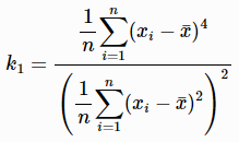\n\n* 若 *biased*=false,表示结果为无偏估计,计算公式为:\n\n\n\n* 若 *X* 为矩阵,计算每列的峰度,返回一个向量。\n\n* 若 *X* 为表,计算每列的峰度,返回一个表。\n\n`kurtosis` 函数也支持校正偏差查询分区表和分布式表。\n\nDolphinDB 的 `kurtosis` 默认情况(当 *biased*=true 时)存在偏差,而 pandas 和 Excel 的 kurt 默认为无偏估计,且减去了正态分布的峰度3。参考下面例子,可以使 DolphinDB 的峰度计算结果与 pandas 和 excel 的结果保持一致:\n\n```\npython\nm = [1111, 323, 43, 51]\ndf = pandas.DataFrame(m)\ny = df.kurt()\n# output\n2.504252\n\ndolphindb\nm=matrix(1111 323 43 51)\nkurtosis(m, false) - 3\n# output\n2.5043\n```\n\n#### 例子\n\n下面的例子使用了 [norm](https://docs.dolphindb.cn/zh/funcs/n/norm.html) 函数生成数据,每次生成的数据都会有细微差别,因此每次计算的结果会有所偏差。\n\n```\nx=norm(0, 1, 1000000);\nkurtosis(x);\n# output\n3.000249\n\nx[0]=100;\nkurtosis(x);\n# output\n100.626722\n\nm=matrix(1..10, 1 2 3 4 5 6 7 8 9 100);\nm;\n```\n\n| #0 | #1 |\n| -- | --- |\n| 1 | 1 |\n| 2 | 2 |\n| 3 | 3 |\n| 4 | 4 |\n| 5 | 5 |\n| 6 | 6 |\n| 7 | 7 |\n| 8 | 8 |\n| 9 | 9 |\n| 10 | 100 |\n\n```\nkurtosis(m);\n# output\n[1.775757575757576,7.997552566718839]\n```\n"
|
|
11561
|
-
},
|
|
11562
|
-
"gaussianNB": {
|
|
11563
|
-
"href": "https://docs.dolphindb.cn/zh/funcs/g/gaussianNB.html",
|
|
11564
|
-
"signatures": [
|
|
11565
|
-
{
|
|
11566
|
-
"full": "gaussianNB(Y, X, [varSmoothing=1e-9])",
|
|
11567
|
-
"name": "gaussianNB",
|
|
11568
|
-
"parameters": [
|
|
11569
|
-
{
|
|
11570
|
-
"full": "Y",
|
|
11571
|
-
"name": "Y"
|
|
11572
|
-
},
|
|
11573
|
-
{
|
|
11574
|
-
"full": "X",
|
|
11575
|
-
"name": "X"
|
|
11576
|
-
},
|
|
11577
|
-
{
|
|
11578
|
-
"full": "[varSmoothing=1e-9]",
|
|
11579
|
-
"name": "varSmoothing",
|
|
11580
|
-
"optional": true,
|
|
11581
|
-
"default": "1e-9"
|
|
11582
|
-
}
|
|
11583
|
-
]
|
|
11584
|
-
}
|
|
11585
|
-
],
|
|
11586
|
-
"markdown": "### [gaussianNB](https://docs.dolphindb.cn/zh/funcs/g/gaussianNB.html)\n\n\n\n#### 语法\n\n`gaussianNB(Y, X, [varSmoothing=1e-9])`\n\n#### 参数\n\n**Y** 是一个长度与 *X* 的行数相等的向量,表示 *X* 中每个样本对应的标签。\n\n**X** 是一个表,表示训练集。表中的每一行表示一个样本,每一列表示一个特征。\n\n**varSmoothing** 是一个浮点类型的正数,表示平滑系数。默认值是 1e-9。\n\n#### 详情\n\n使用高斯朴素贝叶斯(Gaussian Naive Bayes)算法对数据进行分类训练。返回的结果是一个字典,包含以下 key:\n\n* modelName:模型名称,为字符串 \"GaussianNB\"\n\n* model:gaussianNB 的内部模型\n\n* varSmoothing:训练时的平滑系数\n\n#### 例子\n\n本例所用数据集 iris.data 可从 <https://archive.ics.uci.edu/ml/datasets/iris> 下载。\n\n```\nDATA_DIR = \"C:/DolphinDB/Data\"\nt = loadText(DATA_DIR+\"/iris.data\")\nt.rename!(`col0`col1`col2`col3`col4, `sepalLength`sepalWidth`petalLength`petalWidth`class)\nt[`classType] = take(0, t.size())\nupdate t set classType = 1 where class = \"Iris-versicolor\"\nupdate t set classType = 2 where class = \"Iris-virginica\"\n\ntraining = select sepalLength, sepalWidth, petalLength, petalWidth from t\nlabels = t.classType\n\nmodel = gaussianNB(labels, training);\n\npredict(model, training);\n```\n"
|
|
11587
|
-
},
|
|
11588
|
-
"ge": {
|
|
11589
|
-
"href": "https://docs.dolphindb.cn/zh/funcs/g/ge.html",
|
|
11590
|
-
"signatures": [
|
|
11591
|
-
{
|
|
11592
|
-
"full": "ge(X, Y)",
|
|
11593
|
-
"name": "ge",
|
|
11594
|
-
"parameters": [
|
|
11595
|
-
{
|
|
11596
|
-
"full": "X",
|
|
11597
|
-
"name": "X"
|
|
11598
|
-
},
|
|
11599
|
-
{
|
|
11600
|
-
"full": "Y",
|
|
11601
|
-
"name": "Y"
|
|
11602
|
-
}
|
|
11603
|
-
]
|
|
11604
|
-
}
|
|
11605
|
-
],
|
|
11606
|
-
"markdown": "### [ge](https://docs.dolphindb.cn/zh/funcs/g/ge.html)\n\n\n\n#### 语法\n\n`ge(X, Y)` 或 `X>=Y`\n\n#### 参数\n\n**X** 和 **Y** 可以是标量、数据对、向量、矩阵或集合。如果 *X* 或 *Y* 的其中一个是数据对、向量或矩阵,另一个必须是标量,或具有相同长度或维度的数据对、向量或矩阵。\n\n#### 详情\n\n如果 *X* 和 *Y* 都不是集合,返回逐个元素比较 *X*>=*Y* 的结果。\n\n如果 *X* 和 *Y* 都是集合,则检查 *Y* 是否为 *X* 的子集。\n\n#### 例子\n\n*X* 是向量:\n\n```\n1 2 3 >= 2;\n# output\n[0,1,1]\n\n1 2 3 >= 0 2 4;\n# output\n[1,1,0]\n\n2:3>=1:6;\n# output\n1 : 0\n\nm1=1..6$2:3;\nm1;\n```\n\n| #0 | #1 | #2 |\n| -- | -- | -- |\n| 1 | 3 | 5 |\n| 2 | 4 | 6 |\n\n```\nm1 ge 4;\n```\n\n| #0 | #1 | #2 |\n| -- | -- | -- |\n| 0 | 0 | 1 |\n| 0 | 1 | 1 |\n\n```\nm2=6..1$2:3;\nm2;\n```\n\n| #0 | #1 | #2 |\n| -- | -- | -- |\n| 6 | 4 | 2 |\n| 5 | 3 | 1 |\n\n```\nm1>=m2;\n```\n\n| #0 | #1 | #2 |\n| -- | -- | -- |\n| 0 | 0 | 1 |\n| 0 | 1 | 1 |\n\n集合操作:如果 *X*>=*Y*,则 *Y* 是 *X* 的子集。\n\n```\nx=set(4 6);\nx;\n# output\nset(6,4)\ny=set(8 9 4 6);\ny;\n# output\nset(6,4,9,8)\n\ny>=x;\n# output\n1\n\nx>=y;\n# output\n0\n\nx>=x;\n# output\n1\n// x 是 x 的子集\n```\n"
|
|
11607
|
-
},
|
|
11608
|
-
"gema": {
|
|
11609
|
-
"href": "https://docs.dolphindb.cn/zh/funcs/g/gema.html",
|
|
11610
|
-
"signatures": [
|
|
11611
|
-
{
|
|
11612
|
-
"full": "gema(X, window, alpha)",
|
|
11613
|
-
"name": "gema",
|
|
11614
|
-
"parameters": [
|
|
11615
|
-
{
|
|
11616
|
-
"full": "X",
|
|
11617
|
-
"name": "X"
|
|
11618
|
-
},
|
|
11619
|
-
{
|
|
11620
|
-
"full": "window",
|
|
11621
|
-
"name": "window"
|
|
11622
|
-
},
|
|
11623
|
-
{
|
|
11624
|
-
"full": "alpha",
|
|
11625
|
-
"name": "alpha"
|
|
11626
|
-
}
|
|
11627
|
-
]
|
|
11628
|
-
}
|
|
11629
|
-
],
|
|
11630
|
-
"markdown": "### [gema](https://docs.dolphindb.cn/zh/funcs/g/gema.html)\n\n\n\n#### 语法\n\n`gema(X, window, alpha)`\n\nTA-lib 系列函数参数说明和窗口计算规则请参考: [TA-lib 系列](https://docs.dolphindb.cn/zh/funcs/themes/TAlib.html)\n\n#### 参数\n\n**alpha** 是一个0-1之间的浮点数(不包含0, 1),表示计算系数。\n\n#### 详情\n\n在给定长度(以元素个数衡量)的滑动窗口内,计算 *X* 的指数移动平均(Exponential Moving Average),该函数是 [ema](https://docs.dolphindb.cn/zh/funcs/e/ema.html) 的扩展。\n\n与 [ema](https://docs.dolphindb.cn/zh/funcs/e/ema.html) 相比,该函数引入了计算系数 *alpha*,其计算公式为:\n\n\n\n其中:为第 k 个指数移动平均值,alpha 为计算系数,为向量中第 k 个元素。\n\n#### 例子\n\n```\nx=12.1 12.2 12.6 12.8 11.9 11.6 11.2\ngema(x,3,0.5);\n# output\n[,,12.299999999999998,12.55,12.225000000000001,11.912500000000001,11.55625]\n\nx=matrix(12.1 12.2 12.6 12.8 11.9 11.6 11.2, 14 15 18 19 21 12 10)\ngema(x,3,0.1);\n```\n\n| col1 | col2 |\n| ------- | ------- |\n| | |\n| | |\n| 12.3 | 15.6667 |\n| 12.35 | 16 |\n| 12.305 | 16.5 |\n| 12.2345 | 16.05 |\n| 12.131 | 15.445 |\n\n相关函数:[ema](https://docs.dolphindb.cn/zh/funcs/e/ema.html), [wilder](https://docs.dolphindb.cn/zh/funcs/w/wilder.html), [tema](https://docs.dolphindb.cn/zh/funcs/t/tema.html)\n"
|
|
11631
|
-
},
|
|
11632
|
-
"genericStateIterate": {
|
|
11633
|
-
"href": "https://docs.dolphindb.cn/zh/funcs/g/genericStateIterate.html",
|
|
11634
|
-
"signatures": [
|
|
11635
|
-
{
|
|
11636
|
-
"full": "genericStateIterate(X, initial, window, func)",
|
|
11637
|
-
"name": "genericStateIterate",
|
|
11638
|
-
"parameters": [
|
|
11639
|
-
{
|
|
11640
|
-
"full": "X",
|
|
11641
|
-
"name": "X"
|
|
11642
|
-
},
|
|
11643
|
-
{
|
|
11644
|
-
"full": "initial",
|
|
11645
|
-
"name": "initial"
|
|
11646
|
-
},
|
|
11647
|
-
{
|
|
11648
|
-
"full": "window",
|
|
11649
|
-
"name": "window"
|
|
11650
|
-
},
|
|
11651
|
-
{
|
|
11652
|
-
"full": "func",
|
|
11653
|
-
"name": "func"
|
|
11654
|
-
}
|
|
11655
|
-
]
|
|
11656
|
-
}
|
|
11657
|
-
],
|
|
11658
|
-
"markdown": "### [genericStateIterate](https://docs.dolphindb.cn/zh/funcs/g/genericStateIterate.html)\n\n\n\n#### 语法\n\n`genericStateIterate(X, initial, window, func)`\n\n#### 参数\n\n**X** 表中的字段或对表字段其应用向量函数的计算结果。通过元组方式传入多个列字段。传入 \\[] 表示不指定该参数。\n\n**initial** 表中的字段或对表字段应用向量函数的计算结果。其作用是对输出表的第1\\~*window* 个计算结果进行填充。\n\n**window**非负整数,表示窗口的长度(以元素个数衡量)。\n\n**func** 用户自定义的无状态函数,其返回值必须是标量,以部分应用的方式接收参数。当 *window* > 0 时,其第一个参数为当前记录向前取 *window* 个计算结果组成的向量;当 *window* = 0 时,其第一个参数为当前记录向前取1个计算结果。其后参数依次为 *X* 指定的列。\n\n#### 详情\n\n基于以元素个数衡量的窗口进行迭代计算。\n\n假设 *X* 指定为 \\[X1, X2, ..., Xn],该函数计算结果对应输出表中的列为 factor,初始化字段为 initial,*window* 为 w,迭代函数为 func。\n\n对于输入的第 k 条记录(k = 1, 2 …),其计算逻辑为:\n\n* 当 w = 0 时:\n\n * k = 1 时:factor\\[0] = func(initial\\[0],, X1\\[0], X2\\[0], … , Xn\\[0])\n\n * k > 1 时:factor\\[k-1] = func(factor\\[(k-2)], X1\\[k-1], X2\\[k-1], … , Xn\\[k-1])\n\n* 当 w >0 时:\n\n * k <= w 时:factor\\[k-1] = initial\\[k-1]\n * k > w 时:factor\\[k-1] = func(factor\\[(k-1-w):k-1], X1\\[k-1], X2\\[k-1], … , Xn\\[k-1])\n\n注意:数据对用于索引时,不包含右边界的值,即 (k-1-w):k-1 的范围是 \\[k-1-w, k-1)。\n\n#### 例子\n\n```\n// define a function\ndef myfunc(x, w){ \nre = sum(x*w)\nreturn re\n}\n\ndateTime = 2021.09.09T09:30:00.000 2021.09.09T09:31:00.000 2021.09.09T09:32:00.000 2021.09.09T09:33:00.000 2021.09.09T09:34:00.000\nsecurityID = `600021`600021`600021`600021`600021\nvolume = 310 280 300 290 240\nprice = 1.5 1.6 1.7 1.6 1.5\nt = table(1:0, `dateTime`securityID`volume`price, [TIMESTAMP, SYMBOL, INT, DOUBLE])\ntableInsert(t, dateTime, securityID, volume, price)\noutput = table(100:0, `securityID`dateTime`factor1, [SYMBOL, TIMESTAMP, DOUBLE])\n\nengine = createReactiveStateEngine(name=\"test\", metrics=[<dateTime>, <genericStateIterate(volume,price,3,myfunc{,})>], dummyTable=t, outputTable=output, keyColumn=`SecurityID, keepOrder=true)\nengine.append!(t)\ndropAggregator(`test)\n```\n\n| securityID | dateTime | factor1 |\n| ---------- | ----------------------- | ------- |\n| 600021 | 2021.09.09T09:30:00.000 | 1.5 |\n| 600021 | 2021.09.09T09:31:00.000 | 1.6 |\n| 600021 | 2021.09.09T09:32:00.000 | 1.7 |\n| 600021 | 2021.09.09T09:33:00.000 | 1,392 |\n| 600021 | 2021.09.09T09:34:00.000 | 334,872 |\n\n上例计算过程如下:\n\n* 由于窗口为 3,因此对于前 3 条数据,以 price 的值作为 factor1 的输出;\n\n* 第 4 条数据到来时,历史窗口的数据为 \\[1.5, 1.6, 1.7],当前 volume 的值为 290,因此调用自定义函数 myfunc(\\[1.5, 1.6, 1.7], 290) = 1392;\n\n* 第 5 条数据到来时,历史窗口的数据为 \\[1.6, 1.7, 1392],当前 volume 的值为 240,因此调用自定义函数 myfunc(\\[1.6, 1.7, 1392], 240) = 334872;\n\n* 若之后继续有数据注入,其计算过程以此类推。\n\n相关函数:[genericTStateIterate](https://docs.dolphindb.cn/zh/funcs/g/genericTStateIterate.html)\n"
|
|
11659
|
-
},
|
|
11660
|
-
"genericTStateIterate": {
|
|
11661
|
-
"href": "https://docs.dolphindb.cn/zh/funcs/g/genericTStateIterate.html",
|
|
11662
|
-
"signatures": [
|
|
11663
|
-
{
|
|
11664
|
-
"full": "genericTStateIterate(T, X, initial, window, func, [leftClosed = false])",
|
|
11665
|
-
"name": "genericTStateIterate",
|
|
11666
|
-
"parameters": [
|
|
11667
|
-
{
|
|
11668
|
-
"full": "T",
|
|
11669
|
-
"name": "T"
|
|
11670
|
-
},
|
|
11671
|
-
{
|
|
11672
|
-
"full": "X",
|
|
11673
|
-
"name": "X"
|
|
11674
|
-
},
|
|
11675
|
-
{
|
|
11676
|
-
"full": "initial",
|
|
11677
|
-
"name": "initial"
|
|
11678
|
-
},
|
|
11679
|
-
{
|
|
11680
|
-
"full": "window",
|
|
11681
|
-
"name": "window"
|
|
11682
|
-
},
|
|
11683
|
-
{
|
|
11684
|
-
"full": "func",
|
|
11685
|
-
"name": "func"
|
|
11686
|
-
},
|
|
11687
|
-
{
|
|
11688
|
-
"full": "[leftClosed = false]",
|
|
11689
|
-
"name": "[leftClosed = false]"
|
|
11690
|
-
}
|
|
11691
|
-
]
|
|
11692
|
-
}
|
|
11693
|
-
],
|
|
11694
|
-
"markdown": "### [genericTStateIterate](https://docs.dolphindb.cn/zh/funcs/g/genericTStateIterate.html)\n\n\n\n#### 语法\n\n`genericTStateIterate(T, X, initial, window, func, [leftClosed = false])`\n\n#### 参数\n\n**T** 非严格递增的时间类型或整型的向量,且不能包含 NULL 值。注意,时间乱序的数据在计算中会被直接丢弃。\n\n**X** 表中的字段或对其应用向量函数的计算结果。若不指定,需要置为\\[];若需要输入多个列变量,需要用元组表示。\n\n**initial** 用于初始化的列字段,作为初始化窗口内元素的输出,初始化窗口为 \\[t0, t0 + *window*)(t0 为第一条数据的时间戳,以时间衡量窗口)。*initial* 可以是输入表中的字段或对其应用向量函数的计算结果。\n\n**window** 正整型或 DURATION 标量,表示初始化窗口和历史窗口的长度。当 *window* 为整数时,其单位与 T 一致。\n\n**func** 无状态函数,为用户自定义函数,其返回值必须是标量。以部分应用的形式传入。*func* 参数个数为 1(历史窗口内的数据)+ *X* 指定的列数,第一个参数对应历史窗口的元素值,之后的参数依次对应 X *指定列的元素值*。除前述参数外,若 *func* 包含其他固定的常量参数,则需以部分应用的形式指定。\n\n**leftClosed** 布尔值,表示历史窗口是否包含左边界的数据,默认为 false。\n\n#### 详情\n\n基于以时间衡量的窗口进行迭代计算。\n\n假设时间列为 *T*,*X* 指定为 \\[X1, X2, ..., Xn],该函数计算结果对应输出表中的列为 factor,初始化字段为 *initial*,*window* 为 w,迭代函数为 func。\n\n以 Tk 表示第 k 条数据的时间戳,对于第 k 条记录(k = 1, 2 ...),其计算逻辑为:\n\n* Tk ∈ \\[T1, T1+w):factor\\[k] = initial\\[k]\n\n* 其他情况下,第 k+1 条记录对应的窗口为 (Tk-w, Tk] (leftClosed=false) / \\[Tk-w, Tk] (leftClosed=true):factor\\[k] = func(subFactor, X1\\[k], X2\\[k], ... , Xn\\[k]),其中 subFactor 为当前窗口范围内 factor 的值。\n\n**Note:**\n\n数据对用于索引时,不包含右边界的值,即 (k-w):k 的范围是 \\[k-w, k)。\n\n#### 例子\n\n指定 *leftClosed*=false:\n\n```\n// define a function\ndef myfunc(x, w){ \n re = sum(x*w)\n return re\n }\n\ndateTime = 2021.09.09T09:28:00.000 2021.09.09T09:28:30.000 2021.09.09T09:30:00.000 2021.09.09T09:31:00.000 2021.09.09T09:32:00.000\nsecurityID = `600021`600021`600021`600021`600021\nvolume = 310 280 300 290 240\nprice = 1.5 1.6 1.7 1.6 1.5\nt = table(1:0, `dateTime`securityID`volume`price, [TIMESTAMP, SYMBOL, INT, DOUBLE])\ntableInsert(t, dateTime, securityID, volume, price)\noutput = table(100:0, `securityID`dateTime`factor1, [SYMBOL, TIMESTAMP, DOUBLE])\n\nengine = createReactiveStateEngine(name=\"test\", metrics=[<dateTime>, <genericTStateIterate(dateTime,volume,price,2m,myfunc{,})>], dummyTable=t, outputTable=output, keyColumn=`SecurityID, keepOrder=true)\nengine.append!(t)\ndropAggregator(`test)\n```\n\n| securityID | dateTime | factor1 |\n| ---------- | ----------------------- | ---------- |\n| 600021 | 2021.09.09T09:28:00.000 | 1.5 |\n| 600021 | 2021.09.09T09:28:30.000 | 1.6 |\n| 600021 | 2021.09.09T09:30:00.000 | 930 |\n| 600021 | 2021.09.09T09:31:00.000 | 270,164 |\n| 600021 | 2021.09.09T09:32:00.000 | 65,062,560 |\n\n上例计算过程如下:\n\n* 由于第 1 条数据的时间戳为 09:28:00.000 窗口为 2 min,因此初始化窗口为 \\[2021.09.09T09:28:00.000, 2021.09.09T09:30:00.000),前 2 条数据均属于该窗口,因此直接输出 price 的值。\n\n* 第 3 条记录对应的窗口为 (2021.09.09T09:26:30.000, 2021.09.09T09:28:30.000],该历史窗口内的元素为 \\[1.5, 1.6],当前 volume 的值为 300,因此调用自定义函数 myfunc(\\[1.5, 1.6], 300) = 930;\n\n* 同理第 4 条记录对应的窗口为 (2021.09.09T09:28:00.000, 2021.09.09T09:30:00.000],该历史窗口内的元素为 \\[1.6, 930],当前 volume 的值为 290,因此调用自定义函数 myfunc(\\[1.6, 930], 290) = 270164;\n\n* 以此类推。\n\n指定 *leftClosed*=true:\n\n```\nengine = createReactiveStateEngine(name=\"test\", metrics=[<dateTime>, <genericTStateIterate(dateTime,volume,price,2m,myfunc{,},true)>], dummyTable=t, outputTable=output, keyColumn=`SecurityID, keepOrder=true)\n```\n\n| securityID | dateTime | factor1 |\n| ---------- | ----------------------- | ---------- |\n| 600021 | 2021.09.09T09:28:00.000 | 1.5 |\n| 600021 | 2021.09.09T09:28:30.000 | 1.6 |\n| 600021 | 2021.09.09T09:30:00.000 | 930 |\n| 600021 | 2021.09.09T09:31:00.000 | 270,599 |\n| 600021 | 2021.09.09T09:32:00.000 | 65,166,960 |\n\n上例计算过程如下:\n\n* 由于第 1 条数据的时间戳为 09:28:00.000 窗口为 2 min,因此初始化窗口为 \\[2021.09.09T09:28:00.000, 2021.09.09T09:30:00.000),前 2 条数据均属于该窗口,因此直接以 price 的值作为 factor1 的输出。\n\n* 第 3 条记录对应的窗口为 \\[2021.09.09T09:26:30.000, 2021.09.09T09:28:30.000],该历史窗口内的元素为 \\[1.5, 1.6],当前 volume 的值为 300,因此调用自定义函数 myfunc(\\[1.5, 1.6], 300) = 930;\n\n* 同理第 4 条记录对应的窗口为 \\[2021.09.09T09:28:00.000, 2021.09.09T09:30:00.000],该历史窗口内的元素为 \\[1.5, 1.6, 930],当前 volume 的值为 290,因此调用自定义函数 myfunc(\\[1.5, 1.6, 930], 290) = 270599;\n\n* 以此类推。\n\n相关函数:[genericStateIterate](https://docs.dolphindb.cn/zh/funcs/g/genericStateIterate.html)\n"
|
|
11695
|
-
},
|
|
11696
|
-
"genOutputColumnsForOBSnapshotEngine": {
|
|
11697
|
-
"href": "https://docs.dolphindb.cn/zh/funcs/g/genoutputcolumnsforobsnapshotengine.html",
|
|
11698
|
-
"signatures": [
|
|
11699
|
-
{
|
|
11700
|
-
"full": "genOutputColumnsForOBSnapshotEngine([basic=true], [time=true], [depth], [tradeDetail=true], [orderDetail=true], [withdrawDetail=true], [orderBookDetailDepth=0], [prevDetail=true])",
|
|
11701
|
-
"name": "genOutputColumnsForOBSnapshotEngine",
|
|
11702
|
-
"parameters": [
|
|
11703
|
-
{
|
|
11704
|
-
"full": "[basic=true]",
|
|
11705
|
-
"name": "basic",
|
|
11706
|
-
"optional": true,
|
|
11707
|
-
"default": "true"
|
|
11379
|
+
"full": "[basic=true]",
|
|
11380
|
+
"name": "basic",
|
|
11381
|
+
"optional": true,
|
|
11382
|
+
"default": "true"
|
|
11708
11383
|
},
|
|
11709
11384
|
{
|
|
11710
11385
|
"full": "[time=true]",
|
|
@@ -15562,6 +15237,331 @@
|
|
|
15562
15237
|
],
|
|
15563
15238
|
"markdown": "### [iterate](https://docs.dolphindb.cn/zh/funcs/i/iterate.html)\n\n\n\n#### 语法\n\n`iterate(init, coeffs, input)`\n\n#### 参数\n\n**init** 是初始值。\n\n**coeffs** 是迭代系数。*init* 和 *coeffs* 的长度必须相同。\n\n**input** 是整型标量,或者是向量。如果 *input* 是整型标量,表示迭代的次数;如果 *input* 是向量,其长度表示迭代的次数,每个元素在每次迭代后都添加到结果中。\n\n#### 详情\n\n* 若 *init*、*coeffs* 与 *input* 均为标量,返回等比数列\\[ *init* \\* *coeffs* , *init* \\* *coeffs* 2, *init* \\* *coeffs*3, ...],其长度为 *input*。\n\n* 若 *init*、*coeffs* 为标量,*input* 为向量,返回数列x,满足以下条件:x\\[0]= *init* \\* *coeffs* + *input* \\[0],x\\[n]=x\\[n-1]\\* *coeffs* + *input* \\[n]。数列x的长度为 *input* 的长度。\n\n* 若 *init*、*coeffs* 为向量,*input* 为标量,返回数列x,满足以下条件:x\\[n]=y(n)\\*\\* *coeffs* , y(n)=y(n-1)\\[1:].append!(x\\[n-1]), y(0)= *init*, x的长度为 *input* 。其中\\*\\*表示点乘,返回两个向量的内积。\n\n* 若 *init*、*coeffs* 与 *input* 均为向量,返回数列x,满足以下条件:x\\[n]=y(n)\\*\\* *coeffs* + *input* \\[n], y(n)=y(n-1)\\[1:].append!(x\\[n-1]), y(0)= *init*。其中\\*\\*表示点乘,返回两个向量的内积。\n\n#### 例子\n\n```\niterate(1, 0.8, 3);\n# output\n[0.8,0.64,0.512]\n// 1*0.8=0.8, 0.8*0.8=0.64, 0.64*0.8=0.512\n\niterate(1, 0.8, 0.1 0.2 0.3);\n# output\n[0.9,0.92,1.036]\n// 1*0.8+0.1=0.9, 0.9*0.8+0.2=0.92, 0.92*0.8+0.3=1.036\n\niterate(1 1, 1 1, 10);\n# output\n[2,3,5,8,13,21,34,55,89,144]\n// 斐波那契数列: 1*1+1*1=2; 1*1+2*1=3; 2*1+3*1=5; 3*1+5*1=8; ... ; 55*1+89*1=144.\n\niterate(1 1, 1 1, 1 2 3 4 5);\n# output\n[3,6,12,22,39]\n// 1*1+1*1+1=3; 1*1+3*1+2=6; 3*1+6*1+3=12; 6*1+12*1+4=22; 12*1+22*1+5=39.\n```\n"
|
|
15564
15239
|
},
|
|
15240
|
+
"kama": {
|
|
15241
|
+
"href": "https://docs.dolphindb.cn/zh/funcs/k/kama.html",
|
|
15242
|
+
"signatures": [
|
|
15243
|
+
{
|
|
15244
|
+
"full": "kama(X, window)",
|
|
15245
|
+
"name": "kama",
|
|
15246
|
+
"parameters": [
|
|
15247
|
+
{
|
|
15248
|
+
"full": "X",
|
|
15249
|
+
"name": "X"
|
|
15250
|
+
},
|
|
15251
|
+
{
|
|
15252
|
+
"full": "window",
|
|
15253
|
+
"name": "window"
|
|
15254
|
+
}
|
|
15255
|
+
]
|
|
15256
|
+
}
|
|
15257
|
+
],
|
|
15258
|
+
"markdown": "### [kama](https://docs.dolphindb.cn/zh/funcs/k/kama.html)\n\n\n\n#### 语法\n\n`kama(X, window)`\n\nTA-lib 系列函数参数说明和窗口计算规则请参考:[TA-lib 系列](https://docs.dolphindb.cn/zh/funcs/themes/TAlib.html)\n\n#### 详情\n\n在给定长度(以元素个数衡量)的滑动窗口内,计算 *X* 的考夫曼自适应移动平均值(Kaufman Adaptive Moving Average)。\n\n#### 例子\n\n```\nx=[51.65, 81.18, 43.37, 11.26, 82.79, 13.4, 81.87, 63.53, 21.28, 94.23]\nkama(x, 5);\n# output\n[,,,,,81.006144,81.009907,80.793626,80.344572,80.456788]\n\nt=table(take(`A`B,10) as sym, rand(100.0,10) as close)\nselect sym, kama(close, 3) as kama from t context by sym;\n```\n\n输出返回:\n\n| sym | kama |\n| --- | --------- |\n| A | |\n| A | |\n| A | |\n| A | 66.342572 |\n| A | 62.500023 |\n| B | |\n| B | |\n| B | |\n| B | 17.376469 |\n| B | 42.27882 |\n"
|
|
15259
|
+
},
|
|
15260
|
+
"kendall": {
|
|
15261
|
+
"href": "https://docs.dolphindb.cn/zh/funcs/k/kendall.html",
|
|
15262
|
+
"signatures": [
|
|
15263
|
+
{
|
|
15264
|
+
"full": "kendall(X, Y)",
|
|
15265
|
+
"name": "kendall",
|
|
15266
|
+
"parameters": [
|
|
15267
|
+
{
|
|
15268
|
+
"full": "X",
|
|
15269
|
+
"name": "X"
|
|
15270
|
+
},
|
|
15271
|
+
{
|
|
15272
|
+
"full": "Y",
|
|
15273
|
+
"name": "Y"
|
|
15274
|
+
}
|
|
15275
|
+
]
|
|
15276
|
+
}
|
|
15277
|
+
],
|
|
15278
|
+
"markdown": "### [kendall](https://docs.dolphindb.cn/zh/funcs/k/kendall.html)\n\n\n\n#### 语法\n\n`kendall(X, Y)`\n\n#### 参数\n\n**X** 一个标量/向量/矩阵/内存表。\n\n**Y** 一个标量/向量/矩阵/内存表。\n\n#### 详情\n\n计算 *X* 和 *Y* 的 Kendall 相关性系数。计算时忽略 NULL 值。\n\n若 *X* 或 *Y* 是矩阵,对每一列执行上述计算,返回一个向量。\n\n如果 *X* 或 *Y* 是内存表,则对表中的每个数值列执行上述计算,非数值列将返回空,结果为一个表。\n\n#### 例子\n\n```\nx = [33,21,46,-11,78,47,18,20,-5,66]\ny = [1,NULL,10,6,10,3,NULL,NULL,5,3]\nkendall(x, y)\n//output\n0.05\n```\n\n如果 *X* 是矩阵,*Y* 可以长度是与 *X* 行数相同的向量,或者是与 *X* 维度相同的矩阵。返回结果是长度与 *X* 列数相同的向量。\n\n```\nm=1..20$10:2\nkendall(m,x)\n//output\n[-0.0222,-0.0222]\n\nn=rand(20,20)$10:2\nkendall(m,n)\n//output\n[0.3865,-0.1591]\n```\n\n如果 *X* 是表,*Y* 可以是长度与 *X* 行数相同的向量,或者是维度与 *X* 相同的表。返回结果是与 *X* 列数相同的向量。\n\n```\nt=table(2..11 as id, \"a\"+string(2..11) as name)\nkendall(t,x)\n```\n\n| id | name |\n| :------ | :--- |\n| -0.0222 | |\n\n```\nt1=table(x as col1, y as col2)\nkendall(t,t1)\n```\n\n| id | name |\n| :------ | :--- |\n| -0.0222 | |\n"
|
|
15279
|
+
},
|
|
15280
|
+
"keyedStreamTable": {
|
|
15281
|
+
"href": "https://docs.dolphindb.cn/zh/funcs/k/keyedStreamTable.html",
|
|
15282
|
+
"signatures": [
|
|
15283
|
+
{
|
|
15284
|
+
"full": "keyedStreamTable(keyColumn, X, [X1], [X2], .....)",
|
|
15285
|
+
"name": "keyedStreamTable",
|
|
15286
|
+
"parameters": [
|
|
15287
|
+
{
|
|
15288
|
+
"full": "keyColumn",
|
|
15289
|
+
"name": "keyColumn"
|
|
15290
|
+
},
|
|
15291
|
+
{
|
|
15292
|
+
"full": "X",
|
|
15293
|
+
"name": "X"
|
|
15294
|
+
},
|
|
15295
|
+
{
|
|
15296
|
+
"full": "[X1]",
|
|
15297
|
+
"name": "X1",
|
|
15298
|
+
"optional": true
|
|
15299
|
+
},
|
|
15300
|
+
{
|
|
15301
|
+
"full": "[X2]",
|
|
15302
|
+
"name": "X2",
|
|
15303
|
+
"optional": true
|
|
15304
|
+
},
|
|
15305
|
+
{
|
|
15306
|
+
"full": ".....",
|
|
15307
|
+
"name": "....."
|
|
15308
|
+
}
|
|
15309
|
+
]
|
|
15310
|
+
},
|
|
15311
|
+
{
|
|
15312
|
+
"full": "keyedStreamTable(keyColumn, capacity:size, colNames, colTypes)",
|
|
15313
|
+
"name": "keyedStreamTable",
|
|
15314
|
+
"parameters": [
|
|
15315
|
+
{
|
|
15316
|
+
"full": "keyColumn",
|
|
15317
|
+
"name": "keyColumn"
|
|
15318
|
+
},
|
|
15319
|
+
{
|
|
15320
|
+
"full": "capacity:size",
|
|
15321
|
+
"name": "capacity:size"
|
|
15322
|
+
},
|
|
15323
|
+
{
|
|
15324
|
+
"full": "colNames",
|
|
15325
|
+
"name": "colNames"
|
|
15326
|
+
},
|
|
15327
|
+
{
|
|
15328
|
+
"full": "colTypes",
|
|
15329
|
+
"name": "colTypes"
|
|
15330
|
+
}
|
|
15331
|
+
]
|
|
15332
|
+
}
|
|
15333
|
+
],
|
|
15334
|
+
"markdown": "### [keyedStreamTable](https://docs.dolphindb.cn/zh/funcs/k/keyedStreamTable.html)\n\n\n\n#### 语法\n\n`keyedStreamTable(keyColumn, X, [X1], [X2], .....)`\n\n或\n\n`keyedStreamTable(keyColumn, capacity:size, colNames, colTypes)`\n\n#### 参数\n\n**keyColumn** 是一个字符串或向量,表示主键。\n\n第一种用法中: *X*, *X1*....是向量。\n\n第二种用法中:\n\n**capacity** 是正整数,表示建表时系统为该表分配的内存(以记录数为单位)。当记录数超过 *capacity* 时,系统会首先会分配 *capacity* 1.2\\~2 倍的新的内存空间,然后复制数据到新的内存空间,最后释放原来的内存。对于规模较大的表,此类操作的内存占用会很高。因此,建议建表时预先分配一个合理的 *capacity*。\n\n**size** 只能是0或1。若 size=0,则建立一个空表;若 size=1,则建立一个只包含1条记录的表,记录初始值如下:\n\n* BOOL 类型默认值为 false;\n\n* 数值类型、时间类型、IPADDR、COMPLEX、POINT 的默认值为 0;\n\n* Literal, INT128 类型的默认值为 NULL。\n\n**colNames** 是字符串向量,表示列名。\n\n**colTypes** 是向量,表示各列的数据类型。自 2.00.11.2 版本起,允许主键外的其它列指定为数组向量类型。\n\n#### 详情\n\n创建键值流数据表。该表的主键不允许包含重复值。主键支持一个或多个字段。\n\n实际应用中,可能由于网络原因,会出现数据重复提交写入的情况;或者在上游采用了多路高可用的方式写入数据。面对上述场景,键值流数据表可以实现流数据的幂等性写入,即多次写入键值相同的数据,其结果与第一次写入的结果相同,从而避免数据重复写入。\n\n需要注意的是,此处的键值唯一性并非全局唯一,而是指内存中数据的唯一性。为流数据表开启持久化,可以设置内存中保留的数据条数,一旦数据条数超过设定的上限,系统将一半旧的数据持久化至磁盘。这种方案确保了内存中数据键值的唯一性,而不是全局唯一性。尽管如此,已足以解决多路写入或网络延迟导致的重复提交写入的问题。\n\n向表中添加新记录时,系统会自动检查新记录的主键值:\n\n* 如果新记录的主键值与内存中已有记录的主键值重复时,已有的记录不会被更新。\n\n* 一次性批量插入新记录时,若有多条记录具有相同的主键值,且该主键值与已有记录的主键值不同,只有第一条记录能成功插入。\n\n#### 例子\n\n第一种用法:\n\n```\nid=`A`B`C`D`E\nx=1 2 3 4 5\nt1=keyedStreamTable(`id, id, x)\nt1;\n```\n\n| id | x |\n| -- | - |\n| A | 1 |\n| B | 2 |\n| C | 3 |\n| D | 4 |\n| E | 5 |\n\n第二种用法:\n\n```\nt2=keyedStreamTable(`id,100:0,`id`x, [INT,INT])\ninsert into t2 values(1 2 3,10 20 30);\nt2;\n```\n\n| id | x |\n| -- | -- |\n| 1 | 10 |\n| 2 | 20 |\n| 3 | 30 |\n\n往表 t2 中插入重复主键值的数据:\n\n```\ninsert into t2 values(3 4 5,35 45 55)\nt2;\n```\n\n| id | x |\n| -- | -- |\n| 1 | 10 |\n| 2 | 20 |\n| 3 | 30 |\n| 4 | 45 |\n| 5 | 55 |\n\n可以看到,id=3 的记录并没有被覆盖。\n\n主键为多个字段:\n\n```\nt=keyedStreamTable(`sym`id,1:0,`sym`id`val,[SYMBOL,INT,DOUBLE])\ninsert into t values(`A`B`C`D`E,5 4 3 2 1,52.1 64.2 25.5 48.8 71.9);\ninsert into t values(`A`B`R`T`Y,5 8 3 2 1,152.3 164.6 125.5 148.8 171.6);\nt;\n```\n\n| sym | id | val |\n| --- | -- | ----- |\n| A | 5 | 52.1 |\n| B | 4 | 64.2 |\n| C | 3 | 25.5 |\n| D | 2 | 48.8 |\n| E | 1 | 71.9 |\n| B | 8 | 164.6 |\n| R | 3 | 125.5 |\n| T | 2 | 148.8 |\n| Y | 1 | 171.6 |\n"
|
|
15335
|
+
},
|
|
15336
|
+
"keyedTable": {
|
|
15337
|
+
"href": "https://docs.dolphindb.cn/zh/funcs/k/keyedTable.html",
|
|
15338
|
+
"signatures": [
|
|
15339
|
+
{
|
|
15340
|
+
"full": "keyedTable(keyColumns, X, [X1], [X2], .....)",
|
|
15341
|
+
"name": "keyedTable",
|
|
15342
|
+
"parameters": [
|
|
15343
|
+
{
|
|
15344
|
+
"full": "keyColumns",
|
|
15345
|
+
"name": "keyColumns"
|
|
15346
|
+
},
|
|
15347
|
+
{
|
|
15348
|
+
"full": "X",
|
|
15349
|
+
"name": "X"
|
|
15350
|
+
},
|
|
15351
|
+
{
|
|
15352
|
+
"full": "[X1]",
|
|
15353
|
+
"name": "X1",
|
|
15354
|
+
"optional": true
|
|
15355
|
+
},
|
|
15356
|
+
{
|
|
15357
|
+
"full": "[X2]",
|
|
15358
|
+
"name": "X2",
|
|
15359
|
+
"optional": true
|
|
15360
|
+
},
|
|
15361
|
+
{
|
|
15362
|
+
"full": ".....",
|
|
15363
|
+
"name": "....."
|
|
15364
|
+
}
|
|
15365
|
+
]
|
|
15366
|
+
},
|
|
15367
|
+
{
|
|
15368
|
+
"full": "keyedTable(keyColumns, capacity:size, colNames, colTypes)",
|
|
15369
|
+
"name": "keyedTable",
|
|
15370
|
+
"parameters": [
|
|
15371
|
+
{
|
|
15372
|
+
"full": "keyColumns",
|
|
15373
|
+
"name": "keyColumns"
|
|
15374
|
+
},
|
|
15375
|
+
{
|
|
15376
|
+
"full": "capacity:size",
|
|
15377
|
+
"name": "capacity:size"
|
|
15378
|
+
},
|
|
15379
|
+
{
|
|
15380
|
+
"full": "colNames",
|
|
15381
|
+
"name": "colNames"
|
|
15382
|
+
},
|
|
15383
|
+
{
|
|
15384
|
+
"full": "colTypes",
|
|
15385
|
+
"name": "colTypes"
|
|
15386
|
+
}
|
|
15387
|
+
]
|
|
15388
|
+
},
|
|
15389
|
+
{
|
|
15390
|
+
"full": "keyedTable(keyColumns, table)",
|
|
15391
|
+
"name": "keyedTable",
|
|
15392
|
+
"parameters": [
|
|
15393
|
+
{
|
|
15394
|
+
"full": "keyColumns",
|
|
15395
|
+
"name": "keyColumns"
|
|
15396
|
+
},
|
|
15397
|
+
{
|
|
15398
|
+
"full": "table",
|
|
15399
|
+
"name": "table"
|
|
15400
|
+
}
|
|
15401
|
+
]
|
|
15402
|
+
}
|
|
15403
|
+
],
|
|
15404
|
+
"markdown": "### [keyedTable](https://docs.dolphindb.cn/zh/funcs/k/keyedTable.html)\n\n\n\n#### 语法\n\n`keyedTable(keyColumns, X, [X1], [X2], .....)`\n\n或\n\n`keyedTable(keyColumns, capacity:size, colNames, colTypes)`\n\n或\n\n`keyedTable(keyColumns, table)`\n\n#### 参数\n\n**keyColumns** 是一个字符串标量或向量,表示主键。主键的数据类型必须属于以下类别: INTEGRAL, TEMPORAL 或 LITERAL。\n\n第一种用法中,*X*, *X1*....是向量。\n\n第二种用法中,\n\n**capacity** 是正整数,表示建表时系统为该表分配的内存(以记录数为单位)。当记录数超过 *capacity* 时,系统会首先会分配 *capacity* 1.2\\~2倍的新的内存空间,然后复制数据到新的内存空间,最后释放原来的内存。对于规模较大的表,此类操作的内存占用会很高。因此,建议建表时预先分配一个合理的 *capacity*。\n\n**size** 只能是0或1。当数据列是 array vector 时,size 只能是0;当数据列是其它类型时,size 可以是0或1。\n\n* 若 *size*=0,则建立一个空表;\n* 若 *size*=1,则建立一个只包含1条记录的表,记录初始值如下:\n * BOOL 类型默认值为 false;\n * 数值类型、时间类型、IPADDR、COMPLEX、POINT 的默认值为 0;\n * Literal, INT128 类型的默认值为 NULL。\n\n**colNames** 是字符串向量,表示列名。\n\n**colTypes** 是向量,表示各列的数据类型。\n\n第三种用法中,`table` 是一个表。注意,*table* 中的 *keyColumns* 不能包含重复值。\n\n#### 详情\n\n创建键值内存表。一个键值内存表有一个主键。主键可由一个或多个字段组成。\n\n向表中添加新记录时,系统会自动检查新记录的主键值,如果新记录的主键值与已有记录的主键值重复时,会更新表中对应的记录。\n\n查询优化:\n\n1. 对于键值内存表,满足以下条件,SQL 查询性能会优于普通内存表:\n\n * SQL语句中只能使用 =, in 或 and, 且 in 谓词使用小于等于两次;\n\n * 查询语句必须包含 *keyColumns* 所有列。\n\n2. 查询 `keyedTable` 时,建议调用 [sliceByKey](https://docs.dolphindb.cn/zh/funcs/s/sliceByKey.html) 以提高性能。\n\n请对比 [索引内存表](https://docs.dolphindb.cn/zh/funcs/i/indexedTable.html) 优化 SQL 查询条件。\n\n具体请参考例3。\n\n**Note:** 该函数不支持创建一个包含 array vector 类型的键值表。\n\n#### 例子\n\n例1. 创建键值表\n\n第一种写法:\n\n```\nsym=`A`B`C`D`E\nid=5 4 3 2 1\nval=52 64 25 48 71\nt=keyedTable(`sym`id,sym,id,val)\nt;\n```\n\n| sym | id | val |\n| --- | -- | --- |\n| A | 5 | 52 |\n| B | 4 | 64 |\n| C | 3 | 25 |\n| D | 2 | 48 |\n| E | 1 | 71 |\n\n第二种写法:\n\n```\nt=keyedTable(`sym`id,1:0,`sym`id`val,[SYMBOL,INT,INT])\ninsert into t values(`A`B`C`D`E,5 4 3 2 1,52 64 25 48 71);\n```\n\n第三种写法:\n\n```\ntmp=table(sym, id, val)\nt=keyedTable(`sym`id, tmp);\n```\n\n创建键值内存分区表:\n\n```\nsym=`A`B`C`D`E\nid=5 4 3 2 1\nval=52 64 25 48 71\nt=keyedTable(`sym`id,sym,id,val)\ndb=database(\"\",VALUE,sym)\npt=db.createPartitionedTable(t,`pt,`sym).append!(t);\n```\n\n例2. 更新键值表\n\n```\nt=keyedTable(`sym,1:0,`sym`datetime`price`qty,[SYMBOL,DATETIME,DOUBLE,DOUBLE])\ninsert into t values(`APPL`IBM`GOOG,2018.06.08T12:30:00 2018.06.08T12:30:00 2018.06.08T12:30:00,50.3 45.6 58.0,5200 4800 7800)\nt;\n```\n\n| sym | datetime | price | qty |\n| ---- | ------------------- | ----- | ---- |\n| APPL | 2018.06.08T12:30:00 | 50.3 | 5200 |\n| IBM | 2018.06.08T12:30:00 | 45.6 | 4800 |\n| GOOG | 2018.06.08T12:30:00 | 58 | 7800 |\n\n插入新记录,并且新记录中的主键值与表中主键值重复:\n\n```\ninsert into t values(`APPL`IBM`GOOG,2018.06.08T12:30:01 2018.06.08T12:30:01 2018.06.08T12:30:01,65.8 45.2 78.6,5800 8700 4600)\nt;\n```\n\n| sym | datetime | price | qty |\n| ---- | ------------------- | ----- | ---- |\n| APPL | 2018.06.08T12:30:01 | 65.8 | 5800 |\n| IBM | 2018.06.08T12:30:01 | 45.2 | 8700 |\n| GOOG | 2018.06.08T12:30:01 | 78.6 | 4600 |\n\n插入新记录,并且新记录中的主键值重复:\n\n```\ninsert into t values(`MSFT`MSFT,2018.06.08T12:30:01 2018.06.08T12:30:01,45.7 56.9,3600 4500)\nt;\n```\n\n| sym | datetime | price | qty |\n| ---- | ------------------- | ----- | ---- |\n| APPL | 2018.06.08T12:30:01 | 65.8 | 5800 |\n| IBM | 2018.06.08T12:30:01 | 45.2 | 8700 |\n| GOOG | 2018.06.08T12:30:01 | 78.6 | 4600 |\n| MSFT | 2018.06.08T12:30:01 | 56.9 | 4500 |\n\n主键不允许更新:\n\n```\nupdate t set sym=\"C_\"+sym;\n// output: Can't update a key column.\n```\n\n例3. 查询键值内存表\n\n当过滤条件不使用 or,包含所有 *keyColumns*,并且每个条件都使用了等值谓词(=)或 in 谓词,且 in 谓词数量不超过两个时,键值内存表的查询性能优于普通内存表。\n\n以下例子将比较键值内存表和普通内存表的查询性能。首先,分别创建包含100万条记录的普通内存表 t 和键值内存表 kt。\n\n```\nid=shuffle(1..1000000)\ndate=take(2012.06.01..2012.06.10, 1000000)\ntype=rand(9, 1000000)\nval=rand(100.0, 1000000)\nt=table(id, date, type, val)\nkt=keyedTable(`id`date`type, id, date, type, val);\n```\n\n例3.1\n\n```\ntimer(100) select * from t where id=500000, date=2012.06.01, type=0;\n// output: Time elapsed: 161.574 ms\n\ntimer(100) select * from kt where id=500000, date=2012.06.01, type=0;\n// output: Time elapsed: 1.483 ms\n\ntimer(100) sliceByKey(t1, (500000, 2012.06.01, 0))\n// output: Time elapsed: 0.705 ms\n```\n\n例3.2\n\n```\ntimer(100) select * from t where id in [1, 500000], date in 2012.06.01..2012.06.05, type=5;\n// output: Time elapsed: 894.241 ms\n\ntimer(100) select * from kt where id in [1, 500000], date in 2012.06.01..2012.06.05, type=5;\n// output: Time elapsed: 2.322 ms\n```\n\nin 谓词数量超过两个时,键值内存表不会进行查询优化:\n\n例3.3\n\n```\ntimer(100) select * from t where id in [1, 500000], date in 2012.06.01..2012.06.05, type in 1..5;\n// output: Time elapsed: 801.347 ms\n\ntimer(100) select * from kt where id in [1, 500000], date in 2012.06.01..2012.06.05, type in 1..5;\n// output: Time elapsed: 834.184 ms\n```\n\n若过滤条件没有包括所有 *keyColumns*,键值内存表亦不会进行查询优化:\n\n例3.4\n\n```\ntimer(100) select * from t where id=500000, date in 2012.06.01..2012.06.05;\n// output: Time elapsed: 177.113 ms\n\ntimer(100) select * from kt where id=500000, date in 2012.06.01..2012.06.05;\n// output: Time elapsed: 163.265 ms\n```\n\n例4. 使用 `keyedTable` 保留每只股票卖方委托的最新五档报价。\n\n```\nsym=[\"a\",\"b\",\"c \"] \ntime=22:58:52.827 22:58:53.627 22:58:53.827 \nvolume=array(INT[]).append!([[100,110,120,115,125],[200,230,220,225,230],[320,300,310,315,310]])\nprice=array(DOUBLE[]).append!([[10.5,10.6,10.7,10.77,10.85],[8.6,8.7,8.76,8.83,8.9],[6.3,6.37,6.42,6.48,6.52]])\nt=keyedTable(`sym,sym,time,volume,price)\nt\n```\n\n<table id=\"table_lr3_2wt_x1c\"><thead><tr><th>\n\nsym\n\n</th><th>\n\ntime\n\n</th><th>\n\nvolume\n\n</th><th>\n\nprice\n\n</th></tr></thead><tbody><tr><td>\n\na\n\n</td><td>\n\n22:58:52.827\n\n</td><td>\n\n\\[100, 110, 120, 115, 125]\n\n</td><td>\n\n\\[10.5, 10.6, 10.7, 10.77, 10.85]\n\n</td></tr><tr><td>\n\nb\n\n</td><td>\n\n22:58:53.627\n\n</td><td>\n\n\\[200, 230, 220, 225, 230]\n\n</td><td>\n\n\\[8.6, 8.7, 8.76, 8.83, 8.9]\n\n</td></tr><tr><td>\n\nc\n\n</td><td>\n\n22:58:53.827\n\n</td><td>\n\n\\[320, 300, 310, 315, 310]\n\n</td><td>\n\n\\[6.3, 6.37, 6.42, 6.48, 6.52]\n\n</td></tr></tbody>\n</table>```\n//最新的报价数量和价格\nnewVolume=array(INT[]).append!([[130,110,110,115,120]])\nnewPrice= array(DOUBLE[]).append!([[10.55,10.57,10.62,10.68,10.5]])\n//更新名为 a 的股票的最新报价\nupdate t set volume=newVolume, price=newPrice where sym=\"a\"\nt\n```\n\n<table id=\"table_qr3_2wt_x1c\"><thead><tr><th>\n\nsym\n\n</th><th>\n\ntime\n\n</th><th>\n\nvolume\n\n</th><th>\n\nprice\n\n</th></tr></thead><tbody><tr><td>\n\na\n\n</td><td>\n\n22:58:52.827\n\n</td><td>\n\n\\[130, 110, 110, 115, 120]\n\n</td><td>\n\n\\[10.55, 10.57, 10.62, 10.68, 10.5]\n\n</td></tr><tr><td>\n\nb\n\n</td><td>\n\n22:58:53.627\n\n</td><td>\n\n\\[200, 230, 220, 225, 230]\n\n</td><td>\n\n\\[8.6, 8.7, 8.76, 8.83, 8.9]\n\n</td></tr><tr><td>\n\nc\n\n</td><td>\n\n22:58:53.827\n\n</td><td>\n\n\\[320, 300, 310, 315, 310]\n\n</td><td>\n\n\\[6.3, 6.37, 6.42, 6.48, 6.52]\n\n</td></tr></tbody>\n</table>需要注意的是,更新 array vector 列的数据时,新记录中各行向量的元素个数必须和原记录中对应行向量的元素个数相同,否则会出现报错。如下例,新记录向量中有4个元素,而已有记录对应行的向量中有5个元素,数量不相同,出现报错:\n\n```\nnewVolume=array(INT[]).append!([[130,110,110,120]])\nnewPrice= array(DOUBLE[]).append!([[10.55,10.57,10.62,10.5]])\n\nupdate t set volume=newVolume, price=newPrice where sym=\"a\"\n// error: Failed to update column: volume\n```\n\n相关函数:[indexedTable](https://docs.dolphindb.cn/zh/funcs/i/indexedTable.html)\n"
|
|
15405
|
+
},
|
|
15406
|
+
"keys": {
|
|
15407
|
+
"href": "https://docs.dolphindb.cn/zh/funcs/k/keys.html",
|
|
15408
|
+
"signatures": [
|
|
15409
|
+
{
|
|
15410
|
+
"full": "keys(X)",
|
|
15411
|
+
"name": "keys",
|
|
15412
|
+
"parameters": [
|
|
15413
|
+
{
|
|
15414
|
+
"full": "X",
|
|
15415
|
+
"name": "X"
|
|
15416
|
+
}
|
|
15417
|
+
]
|
|
15418
|
+
}
|
|
15419
|
+
],
|
|
15420
|
+
"markdown": "### [keys](https://docs.dolphindb.cn/zh/funcs/k/keys.html)\n\n\n\n#### 语法\n\n`keys(X)`\n\n#### 参数\n\n**X** 是一个字典、数据表,或集合。\n\n#### 详情\n\n返回一个字典中的所有键作为一个向量,或一个数据表中的列名作为一个向量,或将一个集合转化为一个向量。\n\n#### 例子\n\n```\nz=dict(INT,DOUBLE)\nz[5]=7.9\nz[3]=6\nz.keys();\n# output\n[3,5]\n\nt = table(1 2 3 as id, 4 5 6 as x, `IBM`MSFT`GOOG as name);\nkeys(t);\n# output\n[\"id\",\"x\",\"name\"]\n\na=set(1 2 4)\na.keys();\n# output\n[4,2,1]\n```\n\n相关函数:[values](https://docs.dolphindb.cn/zh/funcs/v/values.html)\n"
|
|
15421
|
+
},
|
|
15422
|
+
"kmeans": {
|
|
15423
|
+
"href": "https://docs.dolphindb.cn/zh/funcs/k/kmeans.html",
|
|
15424
|
+
"signatures": [
|
|
15425
|
+
{
|
|
15426
|
+
"full": "kmeans(X, k, [maxIter=300], [randomSeed], [init='random'])",
|
|
15427
|
+
"name": "kmeans",
|
|
15428
|
+
"parameters": [
|
|
15429
|
+
{
|
|
15430
|
+
"full": "X",
|
|
15431
|
+
"name": "X"
|
|
15432
|
+
},
|
|
15433
|
+
{
|
|
15434
|
+
"full": "k",
|
|
15435
|
+
"name": "k"
|
|
15436
|
+
},
|
|
15437
|
+
{
|
|
15438
|
+
"full": "[maxIter=300]",
|
|
15439
|
+
"name": "maxIter",
|
|
15440
|
+
"optional": true,
|
|
15441
|
+
"default": "300"
|
|
15442
|
+
},
|
|
15443
|
+
{
|
|
15444
|
+
"full": "[randomSeed]",
|
|
15445
|
+
"name": "randomSeed",
|
|
15446
|
+
"optional": true
|
|
15447
|
+
},
|
|
15448
|
+
{
|
|
15449
|
+
"full": "[init='random']",
|
|
15450
|
+
"name": "init",
|
|
15451
|
+
"optional": true,
|
|
15452
|
+
"default": "'random'"
|
|
15453
|
+
}
|
|
15454
|
+
]
|
|
15455
|
+
}
|
|
15456
|
+
],
|
|
15457
|
+
"markdown": "### [kmeans](https://docs.dolphindb.cn/zh/funcs/k/kmeans.html)\n\n\n\n#### 语法\n\n`kmeans(X, k, [maxIter=300], [randomSeed], [init='random'])`\n\n#### 参数\n\n**X** 是一个表,表示训练集。\n\n**k** 是一个正整数,表示要生成的聚类数。\n\n**maxIter** 是一个正整数,表示质心更新的最大迭代次数。默认值是300。\n\n**randomSeed** 是一个整数,表示质心初始化时随机算法的种子。默认值为 NULL。\n\n**init** 可以是一个字符串或者一个矩阵,表示初始值的选择方式。默认值是 'random'。\n\n* 若 *init* 是一个字符串,则可选参数为 'random' 或 'k-means++'。'random' 表示根据 *randomSeed* 随机生成,'kmeans++' 表示根据 kmeans++ 算法生成。\n\n* 若 *init* 是一个矩阵,表示自定义的质心。其列数与表 *X* 需保持一致,行数为 *k*。\n\n#### 详情\n\n对训练集执行 K-Means 聚类。返回的结果是一个字典,包含以下 key:\n\n* centers:一个 *k* 行 m 列的矩阵(m 是 *X* 的列数),包含各个类的质心坐标。\n\n* predict:一个聚类模型预测函数,数据类型是 FUNCTIONDEF。\n\n* modelName:字符串 'KMeans'。\n\n* model:保存的模型,数据类型为 RESOURCE,用于预测。\n\n* labels:一个向量,表示 *X* 中每一行数据对应的聚类的类标签。\n\n#### 例子\n\n使用模拟数据训练一个 K-Means 模型:\n\n```\nt = table(100:0, `x0`x1, [DOUBLE, DOUBLE])\nx0 = norm(1.0, 1.0, 50)\nx1 = norm(1.0, 1.5, 50)\ninsert into t values (x0, x1)\nx0 = norm(2.0, 1.0, 50)\nx1 = norm(-1.0, 1.5, 50)\ninsert into t values (x0, x1)\nx0 = norm(-1.0, 1.0, 50)\nx1 = norm(-3.0, 1.5, 50)\ninsert into t values (x0, x1);\n\nmodel = kmeans(t, 3);\nmodel;\n\n# output\ncenters->\n\n#0 #1\n--------- ---------\n-1.048027 -3.809539\n1.110899 1.24216\n1.677974 -1.19158\n\npredict->kmeansPredict\nmodelName->KMeans\nmodel->KMeans\nlabels->[2,2,2,2,2,2,3,2,3,2,...]\n```\n"
|
|
15458
|
+
},
|
|
15459
|
+
"knn": {
|
|
15460
|
+
"href": "https://docs.dolphindb.cn/zh/funcs/k/knn.html",
|
|
15461
|
+
"signatures": [
|
|
15462
|
+
{
|
|
15463
|
+
"full": "knn(Y, X, type, nNeighbor, [power=2])",
|
|
15464
|
+
"name": "knn",
|
|
15465
|
+
"parameters": [
|
|
15466
|
+
{
|
|
15467
|
+
"full": "Y",
|
|
15468
|
+
"name": "Y"
|
|
15469
|
+
},
|
|
15470
|
+
{
|
|
15471
|
+
"full": "X",
|
|
15472
|
+
"name": "X"
|
|
15473
|
+
},
|
|
15474
|
+
{
|
|
15475
|
+
"full": "type",
|
|
15476
|
+
"name": "type"
|
|
15477
|
+
},
|
|
15478
|
+
{
|
|
15479
|
+
"full": "nNeighbor",
|
|
15480
|
+
"name": "nNeighbor"
|
|
15481
|
+
},
|
|
15482
|
+
{
|
|
15483
|
+
"full": "[power=2]",
|
|
15484
|
+
"name": "power",
|
|
15485
|
+
"optional": true,
|
|
15486
|
+
"default": "2"
|
|
15487
|
+
}
|
|
15488
|
+
]
|
|
15489
|
+
}
|
|
15490
|
+
],
|
|
15491
|
+
"markdown": "### [knn](https://docs.dolphindb.cn/zh/funcs/k/knn.html)\n\n\n\n#### 语法\n\n`knn(Y, X, type, nNeighbor, [power=2])`\n\n#### 参数\n\n**Y** 是一个长度与X的行数相等的向量,表示X中每个样本对应的标签。\n\n**X** 是一张表,表示训练集。表中的每一行表示一个样本,每一列表示一个特征。\n\n**type** 是一个字符串。它的取值可以是 'regressor' 或 'classifier'。\n\n**nNeighbor** 是一个正整数,表示 K 邻近算法的邻近节点个数。\n\n**power** 是一个正整数,表示闵可夫斯基距离(Minkowski Distance)的参数。默认值是2,表示使用欧几里得距离(Euclidean Distance)。如果 *power*=1,表示使用曼哈顿距离(Manhattan Distance)。\n\n#### 详情\n\n通过 K 邻近算法(暴力搜索法)对表中的数据进行训练。返回的结果是一个字典,包含以下 key:\n\n* nNeighbor:训练时所用的邻近节点个数\n\n* modelName:模型的名称,为字符串 \"KNN\"\n\n* model:内部模型\n\n* power:训练时所用的闵可夫斯基距离\n\n* type:字符串 \"regressor\" 或 \"classifier\"\n\n#### 例子\n\n```\nheight = 158 158 158 160 160 163 163 160 163 165 165 165 168 168 168 170 170 170\nweight = 58 59 63 59 60 60 61 64 64 61 62 65 62 63 66 63 64 68\nt=table(height, weight)\nlabels=take(1,7) join take(2,11)\nmodel = knn(labels,t,\"classifier\", 5);\n```\n"
|
|
15492
|
+
},
|
|
15493
|
+
"kroghInterpolate": {
|
|
15494
|
+
"href": "https://docs.dolphindb.cn/zh/funcs/k/kroghinterpolate.html",
|
|
15495
|
+
"signatures": [
|
|
15496
|
+
{
|
|
15497
|
+
"full": "kroghInterpolate(Xi, Yi, X, [der=0])",
|
|
15498
|
+
"name": "kroghInterpolate",
|
|
15499
|
+
"parameters": [
|
|
15500
|
+
{
|
|
15501
|
+
"full": "Xi",
|
|
15502
|
+
"name": "Xi"
|
|
15503
|
+
},
|
|
15504
|
+
{
|
|
15505
|
+
"full": "Yi",
|
|
15506
|
+
"name": "Yi"
|
|
15507
|
+
},
|
|
15508
|
+
{
|
|
15509
|
+
"full": "X",
|
|
15510
|
+
"name": "X"
|
|
15511
|
+
},
|
|
15512
|
+
{
|
|
15513
|
+
"full": "[der=0]",
|
|
15514
|
+
"name": "der",
|
|
15515
|
+
"optional": true,
|
|
15516
|
+
"default": "0"
|
|
15517
|
+
}
|
|
15518
|
+
]
|
|
15519
|
+
}
|
|
15520
|
+
],
|
|
15521
|
+
"markdown": "### [kroghInterpolate](https://docs.dolphindb.cn/zh/funcs/k/kroghinterpolate.html)\n\n\n\n#### 语法\n\n`kroghInterpolate(Xi, Yi, X, [der=0])`\n\n#### 参数\n\n**Xi** 数值向量,表示用于插值的点的 x 坐标。必须是递增序列,不能包含 NULL 值。\n\n**Yi** 数值向量,与 *Xi* 等长,表示用于插值的点的 y 坐标。不能包含 NULL 值。\n\n**X** 数值向量,表示需要求值的点的 x 坐标。不能包含 NULL 值。\n\n**der** 可选参数,非负整数,表示返回值的导数阶数。默认值为 0,表示计算多项式函数本身的值。\n\n#### 详情\n\n对一组点集进行多项式插值,该多项式通过点集中所有的数据点对 (xi, yi)。返回在 X 点处指定导数阶数的多项式估值。\n\n可以额外指定在每个点 xi 处的多个导数值:用户通过重复 xi 值并将导数值指定为连续的 yi 值来实现。\n\n* 当 xi 是唯一值时,yi 为多项式 f(x) 的值。\n\n* 当 xi 出现相同值时,则第一个 yi 是 f(x) 的值,第二个为对应的 xi 的一阶导数值,第三个为对应的 xi 的二阶导数值,依此类推。比如对于输入Xi = \\[0,0,1,1],Yi= \\[1,0,2,3],有 Yi\\[0]=f(0),Yi\\[1]=f'(0),Yi\\[2]=f(1),Yi\\[3]=f'(1)。\n\n#### 例子\n\n以正弦函数为例进行多项式插值,分别计算 xx 点处的多项式估值和其一阶导数值。\n\n```\ndef linspace(start, end, num, endpoint=true){\n\tif(endpoint) return end$DOUBLE\\(num-1), start + end$DOUBLE\\(num-1)*0..(num-1)\n\telse return start + end$DOUBLE\\(num-1)*0..(num-1)\t\n}\n\nx = 0 1 2 3 4 5\ny = sin(x)\nxx = linspace(0.0, 5.0, 10)[1]\nyy=kroghInterpolate(x,y,xx)\nyy;\n\nyy1=kroghInterpolate(x,y,xx,1)\nyy1;\n```\n\nyy 返回值:\n\n\\[0,0.515119011157387,0.898231239576709,0.998548648650381,0.793484053410063,0.354287125066207,-0.188319604452395,-0.678504737959061,-0.969692008469677,-0.958924274663139]\n\nyy1 返回值:\n\n\\[0.885486080979582,0.875967413938641,0.459031117252456,-0.103633680213926,-0.612193041424271,-0.92866822117116,-0.976935666075988,-0.742727014588963,-0.273629096989106,0.320916064615744]\n"
|
|
15522
|
+
},
|
|
15523
|
+
"ksTest": {
|
|
15524
|
+
"href": "https://docs.dolphindb.cn/zh/funcs/k/ksTest.html",
|
|
15525
|
+
"signatures": [
|
|
15526
|
+
{
|
|
15527
|
+
"full": "ksTest(X, Y)",
|
|
15528
|
+
"name": "ksTest",
|
|
15529
|
+
"parameters": [
|
|
15530
|
+
{
|
|
15531
|
+
"full": "X",
|
|
15532
|
+
"name": "X"
|
|
15533
|
+
},
|
|
15534
|
+
{
|
|
15535
|
+
"full": "Y",
|
|
15536
|
+
"name": "Y"
|
|
15537
|
+
}
|
|
15538
|
+
]
|
|
15539
|
+
}
|
|
15540
|
+
],
|
|
15541
|
+
"markdown": "### [ksTest](https://docs.dolphindb.cn/zh/funcs/k/ksTest.html)\n\n\n\n#### 语法\n\n`ksTest(X, Y)`\n\n#### 参数\n\n**X** 是一个数值向量。\n\n**Y** 是一个数值向量。\n\n#### 详情\n\n对 *X* 和 *Y* 进行 Kolmogorov-Smirnov 检验,检验它们是否符合同一个分布。返回的结果是一个字典,包含以下 key:\n\n* ksValue:Kolmogorov-Smirnov 统计量\n\n* pValue:p 值\n\n* D:D 统计量\n\n* method:字符串 \"Two-sample Kolmogorov-Smirnov test\"\n\n#### 例子\n\n```\nx = norm(0.0, 1.0, 50)\ny = norm(0.0, 1.0, 20)\nksTest(x, y);\n\n# output\nksValue->0.739301\npValue->0.645199\nD->0.19\nmethod->Two-sample Kolmogorov-Smirnov test\n```\n"
|
|
15542
|
+
},
|
|
15543
|
+
"kurtosis": {
|
|
15544
|
+
"href": "https://docs.dolphindb.cn/zh/funcs/k/kurtosis.html",
|
|
15545
|
+
"signatures": [
|
|
15546
|
+
{
|
|
15547
|
+
"full": "kurtosis(X, [biased=true])",
|
|
15548
|
+
"name": "kurtosis",
|
|
15549
|
+
"parameters": [
|
|
15550
|
+
{
|
|
15551
|
+
"full": "X",
|
|
15552
|
+
"name": "X"
|
|
15553
|
+
},
|
|
15554
|
+
{
|
|
15555
|
+
"full": "[biased=true]",
|
|
15556
|
+
"name": "biased",
|
|
15557
|
+
"optional": true,
|
|
15558
|
+
"default": "true"
|
|
15559
|
+
}
|
|
15560
|
+
]
|
|
15561
|
+
}
|
|
15562
|
+
],
|
|
15563
|
+
"markdown": "### [kurtosis](https://docs.dolphindb.cn/zh/funcs/k/kurtosis.html)\n\n\n\n#### 语法\n\n`kurtosis(X, [biased=true])`\n\n#### 参数\n\n**X** 是一个向量、矩阵或表。\n\n**biased** 是一个布尔值,表示是否为有偏估计。默认值为 true,表示为有偏估计。\n\n#### 详情\n\n计算 *X* 的峰度。`kurtosis` 函数在计算时会忽略 NULL 值。\n\n* 若 *biased*=true,表示结果为有偏估计,计算公式为:\n\n\n\n* 若 *biased*=false,表示结果为无偏估计,计算公式为:\n\n\n\n* 若 *X* 为矩阵,计算每列的峰度,返回一个向量。\n\n* 若 *X* 为表,计算每列的峰度,返回一个表。\n\n`kurtosis` 函数也支持校正偏差查询分区表和分布式表。\n\nDolphinDB 的 `kurtosis` 默认情况(当 *biased*=true 时)存在偏差,而 pandas 和 Excel 的 kurt 默认为无偏估计,且减去了正态分布的峰度3。参考下面例子,可以使 DolphinDB 的峰度计算结果与 pandas 和 excel 的结果保持一致:\n\n```\npython\nm = [1111, 323, 43, 51]\ndf = pandas.DataFrame(m)\ny = df.kurt()\n# output\n2.504252\n\ndolphindb\nm=matrix(1111 323 43 51)\nkurtosis(m, false) - 3\n# output\n2.5043\n```\n\n#### 例子\n\n下面的例子使用了 [norm](https://docs.dolphindb.cn/zh/funcs/n/norm.html) 函数生成数据,每次生成的数据都会有细微差别,因此每次计算的结果会有所偏差。\n\n```\nx=norm(0, 1, 1000000);\nkurtosis(x);\n# output\n3.000249\n\nx[0]=100;\nkurtosis(x);\n# output\n100.626722\n\nm=matrix(1..10, 1 2 3 4 5 6 7 8 9 100);\nm;\n```\n\n| #0 | #1 |\n| -- | --- |\n| 1 | 1 |\n| 2 | 2 |\n| 3 | 3 |\n| 4 | 4 |\n| 5 | 5 |\n| 6 | 6 |\n| 7 | 7 |\n| 8 | 8 |\n| 9 | 9 |\n| 10 | 100 |\n\n```\nkurtosis(m);\n# output\n[1.775757575757576,7.997552566718839]\n```\n"
|
|
15564
|
+
},
|
|
15565
15565
|
"lasso": {
|
|
15566
15566
|
"href": "https://docs.dolphindb.cn/zh/funcs/l/lasso.html",
|
|
15567
15567
|
"signatures": [
|