bibun 0.0.0
This diff represents the content of publicly available package versions that have been released to one of the supported registries. The information contained in this diff is provided for informational purposes only and reflects changes between package versions as they appear in their respective public registries.
- checksums.yaml +7 -0
- checksums.yaml.gz.sig +3 -0
- data/CHANGELOG.md +7 -0
- data/LICENSE.txt +26 -0
- data/README.md +909 -0
- data/lib/bibun/differential_butcher_table.rb +72 -0
- data/lib/bibun/differential_equation_logger.rb +157 -0
- data/lib/bibun/differential_equation_system.rb +367 -0
- data/lib/bibun/differential_stepper.rb +237 -0
- data/lib/bibun/differential_system_parameter.rb +21 -0
- data/lib/bibun/differential_system_symbol.rb +35 -0
- data/lib/bibun/differential_system_variable.rb +202 -0
- data/lib/bibun/log_entry.rb +131 -0
- data/lib/bibun/step_tracker.rb +129 -0
- data/lib/bibun/symbol_group.rb +100 -0
- data/lib/bibun/version.rb +6 -0
- data/lib/bibun.rb +22 -0
- data/lib/data/butcher_tables.toml +44 -0
- data.tar.gz.sig +0 -0
- metadata +255 -0
- metadata.gz.sig +0 -0
data/README.md
ADDED
|
@@ -0,0 +1,909 @@
|
|
|
1
|
+
Bibun (微分: differential, derivative). This gem implements Runge-Kutta explicit numerical methods to integrate systems of multiple ordinary differential equations. For adaptive step size, it currently implements the Dormand-Prince method of order 5(4) which is commonly find as `ode45`, but with additional features and the ability to finely control the integration with plain Ruby.
|
|
2
|
+
|
|
3
|
+
# Quick feature overview
|
|
4
|
+
|
|
5
|
+
Instant example for a single differential equation with one variable representing a electrical circuit $\frac{dI}{dt}=15-3*I$
|
|
6
|
+
|
|
7
|
+
```ruby
|
|
8
|
+
require 'bibun'
|
|
9
|
+
ode = Bibun::DifferentialEquationSystem.new
|
|
10
|
+
ode.add_variable 'current', 'I', rate_function: '15 - 3 * I'
|
|
11
|
+
ode.log_all(4) # logs all variables with 4 decimals
|
|
12
|
+
ode.integrate starting_values: { 'current' => 0, 'time' => 0 }, step_size: 0.02, duration: 1.5
|
|
13
|
+
ode.logger.save_to_file('integration_run.csv')
|
|
14
|
+
```
|
|
15
|
+
|
|
16
|
+
Using the Dormand Prince method of order (4,5). After the initial step size provided, it adapts it to keep the error below the tolerances provided.
|
|
17
|
+
|
|
18
|
+
```Ruby
|
|
19
|
+
ode.add_variable 'current', 'I', unit: 'A' rate_function: '15 - 3 * I', atol: 0.001, rtol: 0.001
|
|
20
|
+
ode.integrate starting_values: { 'current' => 0, 'time' => 0 }, step_size: 0.02, duration: 1.5, adaptive: true
|
|
21
|
+
puts ode.current.value
|
|
22
|
+
```
|
|
23
|
+
|
|
24
|
+
Using an adaptive method, but logging at a specified interval to provide uniform data for graphing (dense output by polynomial interpolation):
|
|
25
|
+
|
|
26
|
+
```Ruby
|
|
27
|
+
ode.add_variable 'current', 'I', unit: 'A' rate_function: '15 - 3 * I', atol: 0.001, rtol: 0.001
|
|
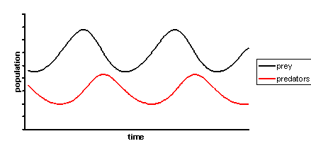
28
|
+
ode.logger.logging_interval = 0.02
|
|
29
|
+
ode.integrate starting_values: { 'current' => 0, 'time' => 0 }, step_size: 0.02, duration: 1.5, adaptive: true
|
|
30
|
+
puts ode.current.value
|
|
31
|
+
```
|
|
32
|
+
|
|
33
|
+
Quick example of a differential equation system of two variables, the Lotka Volterra equations with specific parameter values (p and d are the prey and predator variables):
|
|
34
|
+
$$
|
|
35
|
+
\frac{dp}{dt}=0.08p-0.001pd \\
|
|
36
|
+
\frac{dd}{dt}=-0.02d+0.00001pd
|
|
37
|
+
$$
|
|
38
|
+
|
|
39
|
+
|
|
40
|
+
```RUby
|
|
41
|
+
require 'bibun'
|
|
42
|
+
|
|
43
|
+
# lv stands for a Lotka-Volterra system
|
|
44
|
+
|
|
45
|
+
lv = Bibun::DifferentialEquationSystem.new
|
|
46
|
+
lv.add_variable 'predator', 'd', 'Ecosystem predator', rate_function: '-0.02 * d + 0.00002 * p * d'
|
|
47
|
+
lv.add_variable 'prey', 'p', 'Ecosystem prey', rate_function: '0.08 * p - 0.001 * p * d'
|
|
48
|
+
lv.log_all(2) # Logs all variables with 2 decimals
|
|
49
|
+
lv.integrate starting_values: { 'time' => 0, 'prey' => 1000, 'predator' => 50 }, step_size: 1, duration: 100
|
|
50
|
+
lv.logger.save_to_file('tmp/lotka_volterra_run.csv')
|
|
51
|
+
```
|
|
52
|
+
|
|
53
|
+
The same example as before, but using parameters rather than hard coded numerical values in the formulas:
|
|
54
|
+
|
|
55
|
+
```Ruby
|
|
56
|
+
lv = Bibun::DifferentialEquationSystem.new
|
|
57
|
+
lv.add_variable 'predator', 'd', 'Ecosystem predator', rate_function: '-r * d + b * p * d'
|
|
58
|
+
lv.add_variable 'prey', 'p', 'Ecosystem prey', rate_function: 'k * p - a * p * d'
|
|
59
|
+
lv.add_parameter 'prey_growth', 'k', 'Prey growth rate', value: 0.08
|
|
60
|
+
lv.add_parameter 'prey_consumption', 'a', 'Prey consumption parameter', value: 0.001
|
|
61
|
+
lv.add_parameter 'predator_decay', 'r', 'Predator decay rate', value: 0.02
|
|
62
|
+
lv.add_parameter 'predator_proliferation', 'b', 'Predator proliferation parameter', value: 0.00002
|
|
63
|
+
lv.integrate starting_values: { 'time' => 0, 'prey' => 1000, 'predator' => 50 }, step_size: 1, duration: 100
|
|
64
|
+
```
|
|
65
|
+
|
|
66
|
+
Same example as before, with shortcuts for minimum lines required:
|
|
67
|
+
|
|
68
|
+
```ruby
|
|
69
|
+
lv = Bibun::DifferentialEquationSystem.new
|
|
70
|
+
lv.add_variables({ 'p' => 'k * p - a * p * d', 'd' => '-r * d + b * p * d' })
|
|
71
|
+
lv.add_parameters({ 'k' => 0.08, 'a' => 0.001, 'r' => 0.02, 'b' => 0.00002 })
|
|
72
|
+
lv.integrate starting_values: { 'time' => 0, 'p' => 1000, 'd' => 50 }, step_size: 1, duration: 100
|
|
73
|
+
```
|
|
74
|
+
|
|
75
|
+
The same example as before, but tracking the separate contributions from predation and growth / decay:
|
|
76
|
+
|
|
77
|
+
```Ruby
|
|
78
|
+
lv = Bibun::DifferentialEquationSystem.new
|
|
79
|
+
lv.add_variable 'predator', 'd', 'Ecosystem predator'
|
|
80
|
+
lv.predator.add_rate_term 'Decay', '-r * d'
|
|
81
|
+
lv.predator.add_rate_term 'Predation', 'b * p * d'
|
|
82
|
+
lv.add_variable 'prey', 'p', 'Ecosystem prey'
|
|
83
|
+
lv.prey.add_rate_term 'Growth', 'k * p'
|
|
84
|
+
lv.prey.add_rate_term 'Predation', '- a * p * d'
|
|
85
|
+
lv.add_parameters({ 'k' => 0.08, 'a' => 0.001, 'r' => 0.02, 'b' => 0.00002 })
|
|
86
|
+
lv.log_all(4, with_terms: true) # Shortcut method to adds all variables and their rate terms to the log with 4 decimals
|
|
87
|
+
lv.integrate starting_values: { 'time' => 0, 'prey' => 1000, 'predator' => 50 }, step_size: 1, duration: 100
|
|
88
|
+
# Get array with predator data
|
|
89
|
+
predator_data = lv.logs['predator']
|
|
90
|
+
```
|
|
91
|
+
|
|
92
|
+
With the same basics, a more complex system: an salt tank receiving two inlets, one outlet and variable water volume, proportional loss rate. The concentration is calculated and tracked from the salt mass and volume variables and each flow contribution is tracked separatedly:
|
|
93
|
+
|
|
94
|
+
```mermaid
|
|
95
|
+
---
|
|
96
|
+
title: Interface
|
|
97
|
+
---
|
|
98
|
+
flowchart LR
|
|
99
|
+
tan[Container Tank] -- fo --> out[Outlet]
|
|
100
|
+
bri[Brine inlet cs] -- fb --> tan
|
|
101
|
+
spw[Springwater inlet] -- fw --> tan
|
|
102
|
+
tan -- lV --> los[Loss rate]
|
|
103
|
+
```
|
|
104
|
+
|
|
105
|
+
```Ruby
|
|
106
|
+
tank = Bibun::DifferentialEquationSystem.new
|
|
107
|
+
tank.time.unit = 'h'
|
|
108
|
+
tank.add_variable 'salt', 'm', 'Mass of salt', 'kg', atol: 0.1
|
|
109
|
+
tank.add_variable 'volume', 'V', 'Tank liquid volume', 'm3', atol: 0.1
|
|
110
|
+
tank.add_parameter 'brine_inlet_flow', 'fb', 'Brine intake', 'm3 / h', value: 5
|
|
111
|
+
tank.add_parameter 'brine_concentration', 'cb', 'Brine concentration', 'kg / m3', value: 35
|
|
112
|
+
tank.add_parameter 'water_inlet_flow', 'fw', 'Water intake', 'm3 / h', value: 2
|
|
113
|
+
tank.add_parameter 'outlet_flow', 'fo', 'Outlet flow', 'm3 / h', value: 6
|
|
114
|
+
tank.add_parameter 'loss_coefficient', 'l', 'Loss coefficient rate', 'h-1', value: 0.25
|
|
115
|
+
tank.volume.add_rate_term 'Outlet loss', '-fo'
|
|
116
|
+
tank.volume.add_rate_term 'Brine inlet gain', 'fb'
|
|
117
|
+
tank.volume.add_rate_term 'Springwater inlet gain', 'fw'
|
|
118
|
+
tank.volume.add_rate_term 'Evaporation', '-l * V'
|
|
119
|
+
tank.salt.add_rate_term 'Brine inlet gain', 'cb * fb'
|
|
120
|
+
tank.salt.add_rate_term 'Outlet loss', '-fo * m / V'
|
|
121
|
+
tank.logger.add_step_state
|
|
122
|
+
tank.logger.add_all(4, with_terms: true)
|
|
123
|
+
tank.logger.add_expression('salt_concentration', 'm / V', 4)
|
|
124
|
+
values = { 'volume' => 50, 'time' => 0, 'salt' => 0 }
|
|
125
|
+
tank.integrate starting_values: values, step_size: 1.fdiv(60), duration: 24, adaptive: true
|
|
126
|
+
puts tank.volume.value # 4.0951 asymptotic towards 4.0
|
|
127
|
+
salt_rate_terms = tank.logs['salt:Brine inlet gain'].zip(tank.logs['salt:Outlet loss'])
|
|
128
|
+
pp salt_rate_terms
|
|
129
|
+
tank.logger.save_to_file('tmp/brine_tank.csv')
|
|
130
|
+
```
|
|
131
|
+
|
|
132
|
+
# Gem Description
|
|
133
|
+
|
|
134
|
+
`Bibun` allows to perform integration runs of systems of differential equations through numerical methods such as the traditional fourth-order Runge-Kutta method or the adaptive Dormand-Prince method similar to ode45 in software packages. `Bibun`, however, runs all on Ruby so it gives you the possibility to achieve complete control and access to its processes through standard object manipulation.
|
|
135
|
+
|
|
136
|
+
`Bibun` comes with handy features for engineers like the ability to separate the contribution of different rate additive terms of the differential functions, the ability to monitor custom expressions through the run and the ability to store and load integration conditions to and from JSON and TOML files.
|
|
137
|
+
|
|
138
|
+
This library can handle nonlinear, inhomogeneous and non-autonomous equations, but for the time being it can only handle first-order, explicit systems of differential equations. Convert higher order equations to first order systems before inputting them.
|
|
139
|
+
|
|
140
|
+
## Intention and spirit of the gem
|
|
141
|
+
|
|
142
|
+
The gem is primarily intended for engineers to perform integrations with fully powered Ruby objects which can are amentable to further processing and manipulation with further programming. For this, the interface is intended to be extensive and rich.
|
|
143
|
+
|
|
144
|
+
Math, enthusiasts which like to do quick programming in REPL style or short scripts are acknowledged by provided quick shortcut methods for easy setup in a few lines, but the extensive methods are given greater priority should conflict within both happen.
|
|
145
|
+
|
|
146
|
+
The gem abides to the Ruby philosophy and provides longer, self describing methods which can be understood naturally at first glance rather than acronyms or abbreviatures and uses object orientation rather than an approach of inputing a function with a long list of primitive arguments and obtaining a literal value.
|
|
147
|
+
|
|
148
|
+
## Dependencies
|
|
149
|
+
|
|
150
|
+
This class uses the `keisan` gem to parse and evaluate mathematical expressions in strings. The main criteria to choose it over the `dentaku` gem was the ability to create multiple instances of `Calculator` each one capable of caching its mathematical expression.
|
|
151
|
+
|
|
152
|
+
The gem uses the `json`, `tomlib` and `csv` libraries for importing and exporting integration runs.
|
|
153
|
+
|
|
154
|
+
`Formatador` is used to display a progress bar while doing the integration and for outputting a DES summary.
|
|
155
|
+
|
|
156
|
+
# General Interface and usage
|
|
157
|
+
|
|
158
|
+
The outer `DifferentialEquationSystem` class exposes enough general methods to be able to perform straightforward integration runs, but for a completely control over the integration process it is better to understand and access the inner objects that compose it. Below is the basic interface to a differential equation system object:
|
|
159
|
+
|
|
160
|
+
```mermaid
|
|
161
|
+
---
|
|
162
|
+
title: Interface
|
|
163
|
+
---
|
|
164
|
+
flowchart LR
|
|
165
|
+
sys[System] --shortcut--> vars[variables]
|
|
166
|
+
sys --> syms[syms]
|
|
167
|
+
syms --> vars
|
|
168
|
+
syms --> pars
|
|
169
|
+
sys --shortcut--> pars[parameters]
|
|
170
|
+
vars --> eq[rate_equations]
|
|
171
|
+
vars --shortcut--> rt[terms]
|
|
172
|
+
eq --> rt
|
|
173
|
+
sys --> st[stepper]
|
|
174
|
+
st --> bc[butcher_table]
|
|
175
|
+
sys --> log[logger]
|
|
176
|
+
sys --> tr[tracker]
|
|
177
|
+
```
|
|
178
|
+
|
|
179
|
+
For easier access there are shortcut methods such as System -> Variables or Variable -> Terms even if the strict relationship lies between adjacent classes.
|
|
180
|
+
|
|
181
|
+
## Working example: the Lotka-Volterra equations
|
|
182
|
+
|
|
183
|
+
The Lotka-Volterra equations will be used as the working example for the documentation.
|
|
184
|
+
|
|
185
|
+
The Lotka-Volterra equations model the change across time in the populations of a prey and a predator species:
|
|
186
|
+
$$
|
|
187
|
+
\frac{dp}{dt}=kp-apd \\
|
|
188
|
+
\frac{dd}{dt}=-rd+bpd
|
|
189
|
+
$$
|
|
190
|
+
$p$ and $d$ are the variables for the prey and predator populations and $k$, $a$, $r$ and $b$ are constant parameters or coefficients.
|
|
191
|
+
|
|
192
|
+
This differential equation system is nonlinear and cyclical, with prey and predator population oscillating around their own maximum and minimum and with a phase shift between them.
|
|
193
|
+
|
|
194
|
+
|
|
195
|
+
|
|
196
|
+
## Adding variables
|
|
197
|
+
|
|
198
|
+
To add dependent variables to the system, use the method `add_variable`:
|
|
199
|
+
|
|
200
|
+
```Ruby
|
|
201
|
+
lv.add_variable 'predator', 'd', 'Ecosystem predator', 'individuals', type: :organism, rate_equation: '-0.02 * d - 0.00001 * p * d '
|
|
202
|
+
```
|
|
203
|
+
|
|
204
|
+
The arguments for the method and attributes of the variable are:
|
|
205
|
+
|
|
206
|
+
| Parameter | Required | Argument type | Description |
|
|
207
|
+
| ---------------- | ------------------------------------------------------------ | ------------------------------------------------------------ | ------------------------------------------------------------ |
|
|
208
|
+
| `name` | Yes | String, with ruby method requirements (no spaces, no special characters) | Name of the variable. A instance variable and accessor methods will be created with it. |
|
|
209
|
+
| `symbol` | Optional, but highly recommended | String, without spaces and without math symbols | The symbol that will be used in string formulas. |
|
|
210
|
+
| `title` | Optional | String | A longer title to describe the variable without name restrictions |
|
|
211
|
+
| `unit` | Optional | String | The units of the variable |
|
|
212
|
+
| `type:` | Optional | Symbol | A custom type to group variables. |
|
|
213
|
+
| `rate_equation:` | Optional (but must be provided prior integration) | String | A string which represent the mathematical expression for the derivative of the variable. |
|
|
214
|
+
| `atol:` | Optional (for adaptive methods, it is necessary to provide at least one of `rtol` or `atol`) | Float | Absolute error to be used for the adaptive method |
|
|
215
|
+
| `rtol:` | Optional (for adaptive methods, it is necessary to provide at least one of `rtol` or `atol`) | Float | Relative error to be used for the adaptive method |
|
|
216
|
+
| `accessor: true` | Optional | Boolean | If `true`, creates an instance variable and accessor method with the name provided |
|
|
217
|
+
|
|
218
|
+
`Bibun` uses a name to identify a variable in the `variables` hash during program execution and a shorter symbol to identify it in the string formulas. It uses the `name` provided to create an accessor method and a instance variable automatically for easier acess to the variable. You can skip this behaviour if you want by passing `accessor: false`. You can always access the variable through the `variables` hash accessor method.
|
|
219
|
+
|
|
220
|
+
```ruby
|
|
221
|
+
lv.add_variable 'predator', 'd',
|
|
222
|
+
puts lv.predator.symbol # => 'd'
|
|
223
|
+
# Omit accesor creation
|
|
224
|
+
lv.add_variable 'prey', 'p', create_accessor: false
|
|
225
|
+
puts lv.prey.symbol # => NoMethodError
|
|
226
|
+
puts lv.variables['prey'].symbol # => p
|
|
227
|
+
```
|
|
228
|
+
|
|
229
|
+
For quick math work, you can pass a single ordered argument which will be used as both the name and the symbol. To avoid name collisions with short name methods, the accessor won't be created if you only pass a single ordered argument:
|
|
230
|
+
|
|
231
|
+
```Ruby
|
|
232
|
+
des.add_variable 'y', rate_function: '3 * y**2 + t'
|
|
233
|
+
puts des.x.name # => NoMethodError
|
|
234
|
+
```
|
|
235
|
+
|
|
236
|
+
If you do not need the longer names and other attributes, you can use the shortcut method `add_variables` to add them all in a single call:
|
|
237
|
+
|
|
238
|
+
```ruby
|
|
239
|
+
lv.add_variables({ 'p' => '0.08 * p - 0.001 * p * d',
|
|
240
|
+
'd' => '-0.02 * d + 0.00002 * p * d'})
|
|
241
|
+
```
|
|
242
|
+
|
|
243
|
+
When created, a `DifferentialEquationSystem` object automatically creates a `time` variable with symbol `t` which is used as the independent variable. This can be changed if desired by using the `edit_independent_variable_method`which takes the same arguments of `add_variable` save for those which only apply to dependent variables (`rate_function:`, `atol:`, `rtol:`)
|
|
244
|
+
|
|
245
|
+
```ruby
|
|
246
|
+
des = Bibun::DifferentialEquationSystem.new
|
|
247
|
+
des.edit_independent_variable('x')
|
|
248
|
+
des.x.value = 10
|
|
249
|
+
puts des.x.value # => 10
|
|
250
|
+
```
|
|
251
|
+
|
|
252
|
+
## Adding parameters
|
|
253
|
+
|
|
254
|
+
Although they can be ommited in the simplest cases, most of the time it is desirable to assign values to parameters (quantities that stay the same through the integration) at runtime rather than hard coding them in the formula strings.
|
|
255
|
+
|
|
256
|
+
Parameters can be added using the `add_parameter` method, The first four ordered arguments are the same as those of variables; the additional keyword argument `value:` can be used to assign it at the same time the parameter is created. As with variables, an instance variable and accessor method are created unless you either pass `accessor: false` or provide a single ordered argument. You can always get the parameters through the hash accessor method `parameters`
|
|
257
|
+
|
|
258
|
+
The working example implemented using parameters would look like this:
|
|
259
|
+
|
|
260
|
+
```Ruby
|
|
261
|
+
lv = DifferentialEquationSystem.new
|
|
262
|
+
lv.add_variable 'predator', 'd', 'Ecosystem predator', rate_function: '-r * d + b * p * d'
|
|
263
|
+
lv.add_variable 'prey', 'p', 'Ecosystem prey', rate_function: 'k * p - a * p * d'
|
|
264
|
+
lv.add_parameter 'prey_growth', 'k', 'Prey growth coefficient', value: 0.08
|
|
265
|
+
lv.add_parameter 'prey_consumption', 'a', 'Prey consumption coefficient', value: 0.001
|
|
266
|
+
lv.add_parameter 'predator_decay', 'r', 'Predator decay coefficient', value: 0.02
|
|
267
|
+
lv.add_parameter 'predator_proliferation', 'b', 'Predator proliferation coefficient', value: 0.00002
|
|
268
|
+
```
|
|
269
|
+
|
|
270
|
+
If you do not need the longer names and other attributes, you can use the shortcut method `add_parameters` to add them all in a single line:
|
|
271
|
+
|
|
272
|
+
```ruby
|
|
273
|
+
lv.add_parameters({ 'k' => 0.02, 'a' => 0.001, 'r' => 0.02, 'b' => 0.00001 })
|
|
274
|
+
```
|
|
275
|
+
|
|
276
|
+
## Adding equations
|
|
277
|
+
|
|
278
|
+
An instance of the `SubDifferentialEquation` class is automatically created along its variable and can be accessed through the `DifferentialSystemVariable#rate_equation` accessor.
|
|
279
|
+
|
|
280
|
+
```Ruby
|
|
281
|
+
lv.add_variable 'prey', 'p', rate_function: '-r * d + b * p * d'
|
|
282
|
+
puts lv.prey.rate_equation.rate_function # => '-r * d + b * p * d'
|
|
283
|
+
```
|
|
284
|
+
|
|
285
|
+
Usually this object needs not to be accessed since the mathematical expression of the derivative can be provided using the `rate_function` parameter of the `add_variable` method but is always available if needed:
|
|
286
|
+
|
|
287
|
+
```ruby
|
|
288
|
+
lv.add_variable 'predator', 'd', rate_equation: '0.02 * d - 0.00001 * p * d '
|
|
289
|
+
# Oops, wrong signs, so reedit:
|
|
290
|
+
lv.predator.rate_equation.rate_function = '-0.02 * d + 0.00001 * p * d'
|
|
291
|
+
```
|
|
292
|
+
|
|
293
|
+
The expression of the rate function must be provided with the form $dx_i/dt = f(X)$ and using the symbols previously assigned to the variables and parameters.
|
|
294
|
+
|
|
295
|
+
## Adding rate additive terms
|
|
296
|
+
|
|
297
|
+
There are many situations where a differential equation comprises the sum of several different contributions: for example, in a heat transfer problem one might wish to describe the change in temperature as the sum of one heating contribution and a cooling one, or in a reactor one may wish to distinguish between the rate of generation of a substance and its rate of consumption.
|
|
298
|
+
|
|
299
|
+
Although the most straightforward manner to implement this would be to assign distinct variable to each of these rate additive terms and them having them summed at each step after performing the integration, with `Bibun` you can provide the differential equation that governs a variable's derivative as the sum of separate additive terms rather than one single formula. Use the `DifferentialEquationVariable#add_rate_term` method to add each term with a name for it and its mathematical expression. This method technically resides in the `SubDifferentialEquation` class but the shortcut is equivalent.
|
|
300
|
+
|
|
301
|
+
Using terms, our Lotka-Volterra case would look like this:
|
|
302
|
+
|
|
303
|
+
```Ruby
|
|
304
|
+
lv = DifferentialEquationSystem.new
|
|
305
|
+
lv.add_variable 'predator', 'd', 'Ecosystem predator'
|
|
306
|
+
lv.add_variable 'prey', 'p', 'Ecosystem prey'
|
|
307
|
+
lv.add_parameter 'prey_growth', 'k', 'Prey growth coefficient'
|
|
308
|
+
lv.add_parameter 'prey_consumption', 'a', 'Prey consumption coefficient'
|
|
309
|
+
lv.add_parameter 'predator_decay', 'r', 'Predator decay coefficient'
|
|
310
|
+
lv.add_parameter 'predator_proliferation', 'b', 'Predator proliferation coefficient'
|
|
311
|
+
lv.predator.rate_equation.add_rate_term('decay', '-r * d')
|
|
312
|
+
lv.predator.rate_equation.add_rate_term('predation', 'b * p * d')
|
|
313
|
+
lv.prey.rate_equation.add_rate_term('growth', 'k * p')
|
|
314
|
+
lv.prey.rate_equation.add_rate_term('predation', '-a *p * d')
|
|
315
|
+
```
|
|
316
|
+
|
|
317
|
+
The `add_rate_term` method takes a `name` and a `rate_equation` argument.
|
|
318
|
+
|
|
319
|
+
## Assigning values to variables and parameters
|
|
320
|
+
|
|
321
|
+
Variables need to be given starting values before the integration can be run. The method `DifferentialEquationSystem#assign_values` can be used to pass a hash with both variable and parameter values:
|
|
322
|
+
|
|
323
|
+
```Ruby
|
|
324
|
+
lv.assign_values({ 'prey_growth' => 0.08, 'prey_consumption' => 0.001, 'predator_decay' => 0.02, 'predator_proliferation' => 0.00002, 'predator' => 100, 'prey' => 1000 })
|
|
325
|
+
```
|
|
326
|
+
|
|
327
|
+
You can also assign values by directly accessing the `value` instance variable.
|
|
328
|
+
|
|
329
|
+
```Ruby
|
|
330
|
+
lv.predator.value = 100
|
|
331
|
+
lv.prey_growth.value = 0.08
|
|
332
|
+
lv.prey_consumption.value = 0.001
|
|
333
|
+
# ...
|
|
334
|
+
```
|
|
335
|
+
|
|
336
|
+
As shown later, in the main method `integrate` you can also pass the values as a hash for the `starting_values` parameter:
|
|
337
|
+
|
|
338
|
+
```Ruby
|
|
339
|
+
lv.integrate starting_values: { 'prey_growth' => 0.08, 'prey_consumption' => 0.001, 'predator_decay' => 0.02, 'predator_proliferation' => 0.00002, 'predator' => 100, 'prey' => 1000 } # ...
|
|
340
|
+
```
|
|
341
|
+
|
|
342
|
+
# Performing the integration
|
|
343
|
+
|
|
344
|
+
## Constant step, non adaptive
|
|
345
|
+
|
|
346
|
+
The method `integrate` is the main method to perform the integration, that is, starts a run where the variable values at each step are calculated numerically using a numerical method. The `starting_values:` parameter allows a last chance to introduce initial values; `step_size:` is used to input the desired step size ($h$) and the `duration:` parameter determines the lenght of the run. For a non adaptive method, the total number of steps performed will be total_steps = duration / step_size since the step size is held constant.
|
|
347
|
+
|
|
348
|
+
```Ruby
|
|
349
|
+
lv.integrate starting_values: { 'time' => 0, 'prey' => 1000, 'predator' => 50 }, step_size: 1, duration: 100
|
|
350
|
+
puts lv.prey.value # Value at t = 100
|
|
351
|
+
puts lv.predator.value # Value at t = 100
|
|
352
|
+
```
|
|
353
|
+
|
|
354
|
+
*Note: while it might be tempting to pass the step size argument as a rational value (for example: 1 / 60 for time in minutes when the unit is in hours), rational number operations can slow down the execution by two orders of magnitude. It is recommended to pass the arguement as a float.*
|
|
355
|
+
|
|
356
|
+
The independent variable (time or the custom name provided) gets assigned a default value of 0 if it was not assigned before. The DES instance will raise an error if any other variable or parameter has a nil value at the moment of integration.
|
|
357
|
+
|
|
358
|
+
Long integrations with a lot of variables and parameters can take a significant amount of time to complete. A progress bar made with `Formatador` will be displayed in the CLI output. You can supress it if you wish by passing the keyword argument `display_progress: false`.
|
|
359
|
+
|
|
360
|
+
### Method parameters
|
|
361
|
+
|
|
362
|
+
| Parameter | Attribute location | Argument type | Description |
|
|
363
|
+
| ------------------------ | ------------------------------------------------------------ | ------------------------------------------------------ | ------------------------------------------------------------ |
|
|
364
|
+
| `starting_values:` | Variable and parameter values before integrating can be set separately or with the `assign_values` method. | `Hash{String => Numeric}` | Last chance to pass the values of variables and parameters if they haven't been set. |
|
|
365
|
+
| `step_size:` | `tracker.step_size` | `Numeric` | Assigns the stepsize to be taken. |
|
|
366
|
+
| `duration:` | `tracker.duration` | `Numeric` | Sets the timespan or limit value until which the integration will be run. |
|
|
367
|
+
| `method:` | Passed at method call (optional) | Can be `:rk4`, `:midpoint` and `:dopr45` at the moment | Specifically sets the integration method. If absent, defaults to `:rk4` for non adaptive and `:dopr45` for adaptive. |
|
|
368
|
+
| `adaptive:false` | Passed at method call. | `Boolean` | Sets whether to use an adaptive step size or not. |
|
|
369
|
+
| `display_progress: true` | Passed at method call. | `Boolean` | Specifies whether to print a progress bar to `stdout` or not. |
|
|
370
|
+
|
|
371
|
+
|
|
372
|
+
|
|
373
|
+
## Logging integrations and storing in a file
|
|
374
|
+
|
|
375
|
+
Tracking the evolution of the variables and other quantities across the integration is likely the most important use of a numerical integrator. Depending on the case, only some variables might be important to store to simplify the storage file or, alternatively, it might be that there are different quantities or expressions besides the variables which one might want to track and store for further analysis and inspection.
|
|
376
|
+
|
|
377
|
+
`Bibun` keeps a log that is independent of the variables to easily customize and manipulate it at will. The `logger` object from the DES instance lets you define what you desire to track and record. The logger must be set up before staring the integration. Several different quantities can be set to be recorded with it:
|
|
378
|
+
|
|
379
|
+
- Variables of the DES
|
|
380
|
+
- Additive terms for the variables of the DES
|
|
381
|
+
- Custom mathematical expressions which are functions of the variables and parameters of the DES.
|
|
382
|
+
- The iteration counter, which is akin to the `ROW_NUMBER` function for SQL queries.
|
|
383
|
+
|
|
384
|
+
For the purposes of writing to a `.csv` file, columns are written in the order with which they were added to the logger.
|
|
385
|
+
|
|
386
|
+
## Recording a variable
|
|
387
|
+
|
|
388
|
+
To record variables, use the method `add_variables_to_log` . Provide a hash with the variable names and the decimal places to which the values are going to be rounded.
|
|
389
|
+
|
|
390
|
+
```Ruby
|
|
391
|
+
lv.logger.add_variables({ 'time' => 0 , 'predator' => 1, 'prey' => 1 })
|
|
392
|
+
```
|
|
393
|
+
|
|
394
|
+
If multiple variables share the same decimals, you can use the following shortcut method:
|
|
395
|
+
|
|
396
|
+
```ruby
|
|
397
|
+
# After the decimals comes a variable length parameter list
|
|
398
|
+
lv.logger.add_same_decimals_to_variables(2, 'time', 'predator', 'prey')
|
|
399
|
+
```
|
|
400
|
+
|
|
401
|
+
|
|
402
|
+
|
|
403
|
+
## Recording a rate additive term
|
|
404
|
+
|
|
405
|
+
If the differential equations of the variables where introduced as separate additive terms, they can be recorded individually. To record the contribution of a term to the change of the variable in one step, use the method `DifferentialEquationLogger # add_rate_term`, providing the name of the variable, the name of the rate additive term, and the number of decimals places to round the value.
|
|
406
|
+
|
|
407
|
+
```Ruby
|
|
408
|
+
lv.logger.add_rate_term('prey', 'growth', 2)
|
|
409
|
+
```
|
|
410
|
+
|
|
411
|
+
A variable along its additive terms can be added to the log in a single line with the method `logger#add_variable_with_terms`, passing a single common value for the decimal places:
|
|
412
|
+
|
|
413
|
+
```ruby
|
|
414
|
+
lv.logger.add_variable_with_terms('prey', 2)
|
|
415
|
+
# Equivalent to:
|
|
416
|
+
# lv.logger.add_variables({'prey' => 2})
|
|
417
|
+
# lv.logger.add_rate_term('prey', 'growth', 2)
|
|
418
|
+
# lv.logger.add_rate_term('prey', 'predation', 2)
|
|
419
|
+
```
|
|
420
|
+
|
|
421
|
+
As it will be shown later, in the log the rate additive term are such that the value of the variable at the next row equals the sum of its value in the current row plus all the rate additive terms.
|
|
422
|
+
|
|
423
|
+
## Recording the step number
|
|
424
|
+
|
|
425
|
+
When the step size is not 1, it may be desirable to add a row counter column. `logger.add_step_state` adds this step counter without needing any argument.
|
|
426
|
+
|
|
427
|
+
## Recording a expression
|
|
428
|
+
|
|
429
|
+
Custom calculations that are a function of the DES variables and parameters can be set to be tracked during the integration. To record a custom mathematical expression, use the method `DifferentialEquationLogger # add_expression`, providing the name of the expression, the mathematical formula of the expression, and the number of decimals places to round the value.
|
|
430
|
+
|
|
431
|
+
Make sure the expression name is not the same to any variable name.
|
|
432
|
+
|
|
433
|
+
```Ruby
|
|
434
|
+
lv.logger.add_expression('prey_predator_ratio', 'p / d', 2)
|
|
435
|
+
```
|
|
436
|
+
|
|
437
|
+
## Adding all to the logger
|
|
438
|
+
|
|
439
|
+
For quick cases, `add_all` lets adding all variables to the logger in a single line passing a common value for the decimal places. Using `with_terms: true` includes all rate terms if they were specified.
|
|
440
|
+
|
|
441
|
+
```ruby
|
|
442
|
+
# 3 decimal places for all variables and including all terms
|
|
443
|
+
lv.logger.add_all(3, with_terms: true)
|
|
444
|
+
```
|
|
445
|
+
|
|
446
|
+
This method is available as a shortcut from the DES object as `log_all`
|
|
447
|
+
|
|
448
|
+
```Ruby
|
|
449
|
+
# 3 decimal places for all variables and including all terms
|
|
450
|
+
lv.log_all(3, with_terms: false)
|
|
451
|
+
```
|
|
452
|
+
|
|
453
|
+
## Changing the interval of logging
|
|
454
|
+
|
|
455
|
+
Using small step sizes could result in huge log files and slow performance as logs grow in the memory. One can preserve the precision of smaller step sizes and keep the log light by using a different interval for logging. For example, if time is in seconds and the step size is 1 s but we wish to log results only every 30 seconds, we can adjust it with the `logger#logging_interval` writer method:
|
|
456
|
+
|
|
457
|
+
```ruby
|
|
458
|
+
lv.logger.logging_interval = 30
|
|
459
|
+
```
|
|
460
|
+
|
|
461
|
+
## Exporting the log to a `.csv` file
|
|
462
|
+
|
|
463
|
+
After performing the integration, the method `logger#save_to_file` exports the log of the integration to the provided file path. Column order is that of the order with which the quantities to log were input.
|
|
464
|
+
|
|
465
|
+
```Ruby
|
|
466
|
+
lv.logger.save_to_file('Predation.csv')
|
|
467
|
+
```
|
|
468
|
+
The whole program using all the features would be this:
|
|
469
|
+
|
|
470
|
+
```Ruby
|
|
471
|
+
lv = DifferentialEquationSystem.new
|
|
472
|
+
lv.add_variable 'predator', 'd', 'Ecosystem Predator'
|
|
473
|
+
lv.add_variable 'prey', 'p', 'Ecosystem Prey'
|
|
474
|
+
lv.add_parameter 'prey_growth', 'k', 'Prey growth coefficient'
|
|
475
|
+
lv.add_parameter 'prey_consumption', 'a', 'Prey consumption coefficient'
|
|
476
|
+
lv.add_parameter 'predator_decay', 'r', 'Predator decay coefficient'
|
|
477
|
+
lv.add_parameter 'predator_proliferation', 'b', 'Predator proliferation coefficient'
|
|
478
|
+
lv.prey.rate_equation.add_rate_term('decay', '-r * d')
|
|
479
|
+
lv.prey.rate_equation.add_rate_term('predation', 'b * p * d')
|
|
480
|
+
lv.predator.rate_equation.add_rate_term('growth', 'k * p')
|
|
481
|
+
lv.predator.rate_equation.add_rate_term('predation', '-a *p * d')
|
|
482
|
+
|
|
483
|
+
lv.add_variables_to_log({ 'time' => 0 })
|
|
484
|
+
lv.add_variables_to_log({ 'predator' => 1 })
|
|
485
|
+
lv.logger.add_rate_term('predator', 'decay', 2)
|
|
486
|
+
lv.logger.add_rate_term('predator', 'predation', 2)
|
|
487
|
+
lv.add_variables_to_log({ 'prey' => 1 })
|
|
488
|
+
lv.logger.add_rate_term('prey', 'growth', 2)
|
|
489
|
+
lv.logger.add_rate_term('prey', 'predation', 2)
|
|
490
|
+
lv.logger.add_expression('prey-predator_ratio', 'p / d', 2)
|
|
491
|
+
|
|
492
|
+
lv.assign_values({ 'prey_growth' => 0.08, 'prey_consumption' => 0.001, 'predator_decay' => 0.02, 'predator_proliferation' => 0.00002 })
|
|
493
|
+
lv.integrate starting_values: { 'time' => 0, 'prey' => 1000, 'predator' => 50 }, step_size: 1, duration: 100
|
|
494
|
+
lv.logger.save_to_file('Predation.csv')
|
|
495
|
+
```
|
|
496
|
+
Checking some rows of the generated file:
|
|
497
|
+
|
|
498
|
+
| time | predator | predator - decay | predator - predation | prey | prey - growth | prey - predation | prey-predator ratio |
|
|
499
|
+
| :--: | :------: | :--------------: | :------------------: | :----: | :-----------: | :--------------: | :-----------------: |
|
|
500
|
+
| 37 | 80.8 | -1.63 | 3.5 | 2141.2 | 171.17 | -174.87 | 26.5 |
|
|
501
|
+
| 38 | 82.7 | -1.67 | 3.57 | 2137.5 | 170.72 | -178.41 | 25.86 |
|
|
502
|
+
| 39 | 84.6 | -1.71 | 3.63 | 2129.8 | 169.94 | -181.66 | 25.19 |
|
|
503
|
+
|
|
504
|
+
The sums of the terms for each variable equal the value of the variable for the next step. Here at time 37 we can verify that the value for time 38 for the predator population is $80.8 - 1.63 + 3.5 = 82.67$, showing the separate contributions due to predation and decay.
|
|
505
|
+
|
|
506
|
+
*NOTE: when the logging interval is not equal to the step size, the term logs account for it in order to always represent the total change between two logging rows, so their logged values will differ if the logging interval change.*
|
|
507
|
+
|
|
508
|
+
## Accessing the logs programatically
|
|
509
|
+
|
|
510
|
+
After integrating, you can access the logs through the shortcut `DifferentialEquationSystem#logs[]` or with `logger.logs` using the proper key, which is:
|
|
511
|
+
|
|
512
|
+
- For variables, their `name`
|
|
513
|
+
- For additive rate terms, the variable `name` followed by the term `name` with a semicolon in between. For example: `lv.logs['predator:decay']`
|
|
514
|
+
- For custom expressions, the name provided while creating the entry.
|
|
515
|
+
- For the step, use `des.logs['step']`
|
|
516
|
+
|
|
517
|
+
You can also access the logs of variables and rate additive terms through them. The log will be returned as an array with the value gotten at each logging step. so you can use standard array methods on them.
|
|
518
|
+
|
|
519
|
+
```ruby
|
|
520
|
+
# Get last ten step values
|
|
521
|
+
last_prey_values = lv.logs['prey'].last(10)
|
|
522
|
+
# From the logger
|
|
523
|
+
last_prey_values = lv.logger.logs['prey'].last(10)
|
|
524
|
+
```
|
|
525
|
+
|
|
526
|
+
# Using an adaptive method
|
|
527
|
+
|
|
528
|
+
Passing `adaptive: true` to the `integrate` method uses the fifth order (with 4-order for error evaluation) Dormand Prince method. Several extra arguments must be passed overall. You need to pass error tolerances to at least one dependent variable and you can do it while adding them or later by the accessor methods:
|
|
529
|
+
|
|
530
|
+
```Ruby
|
|
531
|
+
lv.add_variable 'prey', 'p', rate_function: 'k * p - a * p * d', atol: 0.1, rtol: 0.01
|
|
532
|
+
# Alternatively
|
|
533
|
+
lv.prey.atol = 0.1
|
|
534
|
+
lv.prey.rtol = 0.01
|
|
535
|
+
```
|
|
536
|
+
|
|
537
|
+
You can pass only relative or absolute tolerance or both (the stepper will take the sum of both for error evaluation, see formulas below). Variables are inherently created with a value of zero for both tolerances. Failure to assign nonzero tolerances in at least one dependent variable will raise an error when calling the `integrate` method. You can pass tolerances for all variables at once with the `set_global_tolerances` method if you wish, although this is only advisable if they share the same units and order of magnitude:
|
|
538
|
+
|
|
539
|
+
```ruby
|
|
540
|
+
lv.set_global_tolerance 0.1, 0.01 # atol of 0.1 and rtol of 0.01
|
|
541
|
+
```
|
|
542
|
+
|
|
543
|
+
The stepper evaluates the error at each iteration and increases the initial step size given if it the overall error is smaller than the aggregate `err` index or decreases the error and repeats the iteration if the error surpasses the aggregate. Because criteria for calculating the error and changing the step size is not set in stone, `Bibun` uses the following formulas[^1] :
|
|
544
|
+
$$
|
|
545
|
+
err = \sqrt{\frac{1}{N}\sum{(\frac{\Delta}{scale})^2}} \\
|
|
546
|
+
\Delta = x_{5^{th}order}-x_{4^{th}order} \\
|
|
547
|
+
scale = atol+rtol\times max(x_n,x_{n+1})
|
|
548
|
+
$$
|
|
549
|
+
Where N is the number of variables with nonzero tolerance. Step size is decreased and the step performed again if err < 1 and step size is increased otherwise. The size adjustment is done according to:
|
|
550
|
+
$$
|
|
551
|
+
h_{next}=h \times clamp(0.9(\frac{1}{err})^{1/5},1/5, 10)
|
|
552
|
+
$$
|
|
553
|
+
The 0.9 safety factor is a reccomendation by J.C. Butcher[^2] while the 1/5..10 range is a recommendation by W. H. Press.
|
|
554
|
+
|
|
555
|
+
### Using dense output
|
|
556
|
+
|
|
557
|
+
Because an adaptive method is constantly adjusting its step size, the log it produces is unevenly spaced, which might be undesirable in certain circumstances, such as creating a uniform graph or closely monitoring its behaviour. You can adjust the logging interval as you would in the non-adaptive case; if you do, the stepper generates the rows at each interval using a polynomial interpolation of fourth degree. This is known as a dense output.
|
|
558
|
+
|
|
559
|
+
```ruby
|
|
560
|
+
lv.logger.logging_interval = 0.02
|
|
561
|
+
lv.integrate adaptive: true # Uses dense output
|
|
562
|
+
```
|
|
563
|
+
|
|
564
|
+
# Custom control by single step
|
|
565
|
+
|
|
566
|
+
Software packages offer an ability to create events in their own syntax in order to control the integration process, one common example being the ability to interrupt and finish the integration if the values of the variables surpass certain limits.
|
|
567
|
+
|
|
568
|
+
`Bibun` offers the `single_step` method to perform one single step of the integration process. This method take the same arguments than the integrate method, but will only peform the setup of the integration run the first time is called (the `starting_values:` parameter is only taken into account the first time, then ignored for any further calls to `single_step` since variables now depend on the integration proces).
|
|
569
|
+
|
|
570
|
+
Because the `integrate` method simply adds a loop to the basic stepping routine, you can easily set an integration with the `single_step` method and a loop and use Ruby to create any condition or perform any action you want in the middle of the integration.
|
|
571
|
+
|
|
572
|
+
Below are shown several examples of what you can do by using a custom loop along `single step`:
|
|
573
|
+
|
|
574
|
+
```ruby
|
|
575
|
+
# Use a constant step method. Integrate over a day (time is in minutes).Stop integration if a variable crosses a threshold. Preemptive setup is shown.
|
|
576
|
+
reactor.assign_values({'time' => 0, 'chemical_oxygen_demand' => 100, 'oxygen' => 5.0 })
|
|
577
|
+
reactor.step_size = (1/60r).to_f # One minute
|
|
578
|
+
1440.times do # 1 day run
|
|
579
|
+
reactor.single_step # reactor is the DES
|
|
580
|
+
break if reactor.chemical_oxigen_demand < 5
|
|
581
|
+
end
|
|
582
|
+
# For a circuit known to stabilize asynthotically, stop when the maximum difference across the last 10 iterations falls below a threshold.
|
|
583
|
+
while unstable
|
|
584
|
+
circuit.single_step # Circuit is the DES
|
|
585
|
+
last_values = circuit.logs['voltage'].last(10)
|
|
586
|
+
unstable = (last_values.max - last_values.min).abs > 0.1
|
|
587
|
+
end
|
|
588
|
+
# Using an adaptive process, stop if a variables stays below a 50 000 UFC / mL threshold for 10 min.
|
|
589
|
+
1000.times do
|
|
590
|
+
medium.single_step adaptive: true
|
|
591
|
+
ar = medium.logs['time']
|
|
592
|
+
lower_bound = ar.find_index(ar.select {|s| s > ar.last - 10 }.min)
|
|
593
|
+
break if medium.logs['staphylococcus'][lower_bound..-1].none? { |s| s >= 5E4 }
|
|
594
|
+
end
|
|
595
|
+
# Harvest a population extracting certain quantity whenever it grows about a threshold and add feed if it falls below a threshold.
|
|
596
|
+
(365 * 24).times do
|
|
597
|
+
tank.single_step
|
|
598
|
+
tank.shrimp.value -= 5_000 if tank.shrimp.value > 25_000
|
|
599
|
+
tank.daphnia.value += 30_000 if tank.daphnia.value < 40_000
|
|
600
|
+
end
|
|
601
|
+
```
|
|
602
|
+
|
|
603
|
+
# Serialization
|
|
604
|
+
|
|
605
|
+
It might be convenient to save the conditions to perform a integration run when performing many of them. The main class has `to_json` and `from_json` methods to write and read from JSON objects. The look of the previous example as a JSON is the following:
|
|
606
|
+
|
|
607
|
+
```json
|
|
608
|
+
{
|
|
609
|
+
"variables": [
|
|
610
|
+
{
|
|
611
|
+
"name": "predator",
|
|
612
|
+
"symbol": "d",
|
|
613
|
+
"title": "Ecosystem predator",
|
|
614
|
+
"unit": null,
|
|
615
|
+
"terms": [
|
|
616
|
+
{
|
|
617
|
+
"name": "decay",
|
|
618
|
+
"rate_function": "-r * d"
|
|
619
|
+
},
|
|
620
|
+
{
|
|
621
|
+
"name": "predation",
|
|
622
|
+
"rate_function": "b * p * d"
|
|
623
|
+
}
|
|
624
|
+
]
|
|
625
|
+
},
|
|
626
|
+
{
|
|
627
|
+
"name": "prey",
|
|
628
|
+
"symbol": "p",
|
|
629
|
+
"title": "Ecosystem prey",
|
|
630
|
+
"unit": null,
|
|
631
|
+
"terms": [
|
|
632
|
+
{
|
|
633
|
+
"name": "growth",
|
|
634
|
+
"rate_function": "k * p"
|
|
635
|
+
},
|
|
636
|
+
{
|
|
637
|
+
"name": "predation",
|
|
638
|
+
"rate_function": "-a *p * d"
|
|
639
|
+
}
|
|
640
|
+
]
|
|
641
|
+
}
|
|
642
|
+
],
|
|
643
|
+
"parameters": [
|
|
644
|
+
{
|
|
645
|
+
"name": "prey_growth",
|
|
646
|
+
"symbol": "k",
|
|
647
|
+
"title": "Prey growth rate",
|
|
648
|
+
"unit": null,
|
|
649
|
+
"value": 0.08
|
|
650
|
+
},
|
|
651
|
+
{
|
|
652
|
+
"name": "prey_consumption",
|
|
653
|
+
"symbol": "a",
|
|
654
|
+
"title": "Prey predation coefficient",
|
|
655
|
+
"unit": null,
|
|
656
|
+
"value": 0.001
|
|
657
|
+
},
|
|
658
|
+
{
|
|
659
|
+
"name": "predator_decay",
|
|
660
|
+
"symbol": "r",
|
|
661
|
+
"title": "Predator decay rate",
|
|
662
|
+
"unit": null,
|
|
663
|
+
"value": 0.02
|
|
664
|
+
},
|
|
665
|
+
{
|
|
666
|
+
"name": "predator_proliferation",
|
|
667
|
+
"symbol": "b",
|
|
668
|
+
"title": "Predator proliferation coefficient",
|
|
669
|
+
"unit": null,
|
|
670
|
+
"value": 0.00002
|
|
671
|
+
}
|
|
672
|
+
],
|
|
673
|
+
"logging": [
|
|
674
|
+
{
|
|
675
|
+
"type": "variable",
|
|
676
|
+
"variable": "time",
|
|
677
|
+
"decimals": 0
|
|
678
|
+
},
|
|
679
|
+
{
|
|
680
|
+
"type": "variable",
|
|
681
|
+
"variable": "predator",
|
|
682
|
+
"decimals": 2
|
|
683
|
+
},
|
|
684
|
+
{
|
|
685
|
+
"type": "term",
|
|
686
|
+
"term": "decay",
|
|
687
|
+
"variable": "predator",
|
|
688
|
+
"decimals": 2
|
|
689
|
+
},
|
|
690
|
+
{
|
|
691
|
+
"type": "term",
|
|
692
|
+
"term": "predation",
|
|
693
|
+
"variable": "predator",
|
|
694
|
+
"decimals": 2
|
|
695
|
+
},
|
|
696
|
+
{
|
|
697
|
+
"type": "variable",
|
|
698
|
+
"variable": "prey",
|
|
699
|
+
"decimals": 2
|
|
700
|
+
},
|
|
701
|
+
{
|
|
702
|
+
"type": "term",
|
|
703
|
+
"term": "growth",
|
|
704
|
+
"variable": "prey",
|
|
705
|
+
"decimals": 2
|
|
706
|
+
},
|
|
707
|
+
{
|
|
708
|
+
"type": "term",
|
|
709
|
+
"term": "predation",
|
|
710
|
+
"variable": "prey",
|
|
711
|
+
"decimals": 2
|
|
712
|
+
},
|
|
713
|
+
{
|
|
714
|
+
"type": "expression",
|
|
715
|
+
"name": "prey-predator ratio",
|
|
716
|
+
"formula": "p / d",
|
|
717
|
+
"decimals": 2
|
|
718
|
+
}
|
|
719
|
+
],
|
|
720
|
+
"values": {
|
|
721
|
+
"time": 0,
|
|
722
|
+
"predator": 50,
|
|
723
|
+
"prey": 1000
|
|
724
|
+
},
|
|
725
|
+
"simulation_options": {
|
|
726
|
+
"step_size": 1,
|
|
727
|
+
"duration": 100,
|
|
728
|
+
"logging_interval": 5
|
|
729
|
+
}
|
|
730
|
+
}
|
|
731
|
+
```
|
|
732
|
+
|
|
733
|
+
Although variables and parameters are more general and seldom worth skipping, the `logging`, `values` and `integration_options` might be skipped and assigned in the program. Loading is trivial:
|
|
734
|
+
|
|
735
|
+
```Ruby
|
|
736
|
+
lv.from_json(File.read('tmp/lotka_volterra.json'))
|
|
737
|
+
lv.integrate
|
|
738
|
+
```
|
|
739
|
+
|
|
740
|
+
There are also `to_toml` and `from_toml` versions to work with TOML files, which I find more confortable to manually create and edit:
|
|
741
|
+
|
|
742
|
+
```toml
|
|
743
|
+
[[variables]]
|
|
744
|
+
name = "predator"
|
|
745
|
+
symbol = "d"
|
|
746
|
+
title = "Ecosystem predator"
|
|
747
|
+
unit = ""
|
|
748
|
+
|
|
749
|
+
[[variables.terms]]
|
|
750
|
+
name = "decay"
|
|
751
|
+
rate_function = "-r * d"
|
|
752
|
+
|
|
753
|
+
[[variables.terms]]
|
|
754
|
+
name = "predation"
|
|
755
|
+
rate_function = "b * p * d"
|
|
756
|
+
|
|
757
|
+
[[variables]]
|
|
758
|
+
name = "prey"
|
|
759
|
+
symbol = "p"
|
|
760
|
+
title = "Ecosystem prey"
|
|
761
|
+
unit = ""
|
|
762
|
+
|
|
763
|
+
[[variables.terms]]
|
|
764
|
+
name = "growth"
|
|
765
|
+
rate_function = "k * p"
|
|
766
|
+
|
|
767
|
+
[[variables.terms]]
|
|
768
|
+
name = "predation"
|
|
769
|
+
rate_function = "-a *p * d"
|
|
770
|
+
|
|
771
|
+
[[parameters]]
|
|
772
|
+
name = "prey_growth"
|
|
773
|
+
symbol = "k"
|
|
774
|
+
title = "Prey growth rate"
|
|
775
|
+
unit = ""
|
|
776
|
+
value = 0.08
|
|
777
|
+
|
|
778
|
+
[[parameters]]
|
|
779
|
+
name = "prey_consumption"
|
|
780
|
+
symbol = "a"
|
|
781
|
+
title = "Prey consumption coefficient"
|
|
782
|
+
unit = ""
|
|
783
|
+
value = 0.001
|
|
784
|
+
|
|
785
|
+
[[parameters]]
|
|
786
|
+
name = "predator_decay"
|
|
787
|
+
symbol = "r"
|
|
788
|
+
title = "Predator decay rate"
|
|
789
|
+
unit = ""
|
|
790
|
+
value = 0.02
|
|
791
|
+
|
|
792
|
+
[[parameters]]
|
|
793
|
+
name = "predator_proliferation"
|
|
794
|
+
symbol = "b"
|
|
795
|
+
title = "Predator proliferation coefficient"
|
|
796
|
+
unit = ""
|
|
797
|
+
value = 2.0e-05
|
|
798
|
+
|
|
799
|
+
[[logging]]
|
|
800
|
+
type = "variable"
|
|
801
|
+
variable = "time"
|
|
802
|
+
decimals = 0
|
|
803
|
+
|
|
804
|
+
[[logging]]
|
|
805
|
+
type = "variable"
|
|
806
|
+
variable = "predator"
|
|
807
|
+
decimals = 2
|
|
808
|
+
|
|
809
|
+
[[logging]]
|
|
810
|
+
type = "term"
|
|
811
|
+
term = "decay"
|
|
812
|
+
variable = "predator"
|
|
813
|
+
decimals = 2
|
|
814
|
+
|
|
815
|
+
[[logging]]
|
|
816
|
+
type = "term"
|
|
817
|
+
term = "predation"
|
|
818
|
+
variable = "predator"
|
|
819
|
+
decimals = 2
|
|
820
|
+
|
|
821
|
+
[[logging]]
|
|
822
|
+
type = "variable"
|
|
823
|
+
variable = "prey"
|
|
824
|
+
decimals = 2
|
|
825
|
+
|
|
826
|
+
[[logging]]
|
|
827
|
+
type = "term"
|
|
828
|
+
term = "growth"
|
|
829
|
+
variable = "prey"
|
|
830
|
+
decimals = 2
|
|
831
|
+
|
|
832
|
+
[[logging]]
|
|
833
|
+
type = "term"
|
|
834
|
+
term = "predation"
|
|
835
|
+
variable = "prey"
|
|
836
|
+
decimals = 2
|
|
837
|
+
|
|
838
|
+
[[logging]]
|
|
839
|
+
name = "prey-predator ratio"
|
|
840
|
+
type = "expression"
|
|
841
|
+
formula = "p / d"
|
|
842
|
+
decimals = 2
|
|
843
|
+
|
|
844
|
+
[values]
|
|
845
|
+
time = 0
|
|
846
|
+
predator = 50
|
|
847
|
+
prey = 1000
|
|
848
|
+
|
|
849
|
+
[simulation_options]
|
|
850
|
+
step_size = 1
|
|
851
|
+
duration = 100
|
|
852
|
+
logging_interval = 5
|
|
853
|
+
```
|
|
854
|
+
|
|
855
|
+
*NOTE: TOML has no specification for null values andso far the only way is to omit the key-value pair if the value is null. I have not found a library which correctly implements this behaviour. This can cause inconsistencies when exporting to TOML and use immediately for loading. Check for "" assignments in the generated TOML file.*
|
|
856
|
+
|
|
857
|
+
# Subclassing: the general integration method
|
|
858
|
+
|
|
859
|
+
Although the default class might give good functionality, some might desire to inherit from `Bibun::DifferentialEquationSystem` to implement some custom procedures within the calculation of each step. For example, physical systems might want to prevent variables to reach negative values, which can happen at near zero regions with not small enough step sizes. The main loop is conveniently separated into different subroutines which are ideal to override in the subclasses:
|
|
860
|
+
|
|
861
|
+
```ruby
|
|
862
|
+
while syms.ind_var.value < step_tracker.ending_point
|
|
863
|
+
unitary_step
|
|
864
|
+
@progress_bar.increment if display_progress
|
|
865
|
+
end
|
|
866
|
+
|
|
867
|
+
def unitary_step
|
|
868
|
+
# Calculation of the variable changes for the next step
|
|
869
|
+
walk_step
|
|
870
|
+
# Logging the values using those the prior variables values and their changes
|
|
871
|
+
append_log
|
|
872
|
+
# Finally commiting the changes into the variables
|
|
873
|
+
change_variables
|
|
874
|
+
end
|
|
875
|
+
```
|
|
876
|
+
|
|
877
|
+
Lets say we simply want to set variable values to zero if they happen to become negative. We can override `change_variables` in the subclass to set those which became negative to zero for the next iteration.
|
|
878
|
+
|
|
879
|
+
```ruby
|
|
880
|
+
# Subclass
|
|
881
|
+
def change_variables
|
|
882
|
+
super
|
|
883
|
+
variables.each_value do |v|
|
|
884
|
+
v.value = 0 if v.value.negative?
|
|
885
|
+
end
|
|
886
|
+
end
|
|
887
|
+
```
|
|
888
|
+
|
|
889
|
+
# Validation
|
|
890
|
+
|
|
891
|
+
The methods have been validated mostly against differential equations with known analytical solutions and in some cases against tabulated data from book examples or simple steps against Libre Calc software. Specific calculations and criteria for modifying the step size are not set into stone and for the popular `ode45` method the documentation does not disclose it, so I cannot guarantee an exact correspondence with it.
|
|
892
|
+
|
|
893
|
+
So far the numerical methods here are explicit and do not take specific features of the DES into consideration so limitations such as unsuitability for stiff equations or gradual shift of cyclic behaviour over time apply.
|
|
894
|
+
|
|
895
|
+
## Bugs, errors and limitations
|
|
896
|
+
|
|
897
|
+
Although testing has been made to ensure the library performs the integration correctly, it is unavoidable to get errors of mathematical nature with certains inputs (for example, division by zero). The library does not check or takes preemptive action against errors of this nature. Some of the errors of this nature are:
|
|
898
|
+
|
|
899
|
+
- Given the exponential nature of many differential equations, it is frequently the case that variables grow quickly to very high values eventually surpassing the `Float` type maximum. A single wrong sign in the rate functions can trigger this, so check those accordingly if the growth behaviour is unexpected or use a custom loop with a stop condition.
|
|
900
|
+
- Similarly, division by a variable might trigger very large values if such variable approaches zero.
|
|
901
|
+
- Operations with the `Rational` number type are quite slower. Passing a `Rational` number as the step size can cause the integration to take two extra orders of magnitude more time than the float case, so it is recommended to pass floats like `1/60r.to_f`.
|
|
902
|
+
- As of the initial version, I have not tested the changing of the `logging_interval` attribute in the midst of integration because I have not found it likely for it to need manual adjustment. It will trigger inconsistent behaviour for the adaptive method.
|
|
903
|
+
|
|
904
|
+
# Future changes
|
|
905
|
+
|
|
906
|
+
As of the initial release, the `Bibun` gem is likely to undergo changes in order to solidify the best functionality for engineering needs. Some aspects like the core stepping process are probably staying largely unmodified although it might change to accomodate the plans to include the Dormand-Prince 8(5,3) method. The serialization feature is the one most likely to evolve. Changes to the outer methods of the interface that could break the API will be implemented if there's common enough use cases for it until reaching a 1.0 version.
|
|
907
|
+
|
|
908
|
+
[^1]: Numerical Recipes. The Art of Scientific Computing. Third Edition, by W. H. Press
|
|
909
|
+
[^2]: Numerical Methods for Ordinary Differential Equations. Second Edition, by J.C. Butcher.
|