zsplit 1.0.1__tar.gz → 1.0.2__tar.gz
This diff represents the content of publicly available package versions that have been released to one of the supported registries. The information contained in this diff is provided for informational purposes only and reflects changes between package versions as they appear in their respective public registries.
- {zsplit-1.0.1/zsplit.egg-info → zsplit-1.0.2}/PKG-INFO +39 -20
- {zsplit-1.0.1 → zsplit-1.0.2}/README.md +38 -19
- {zsplit-1.0.1 → zsplit-1.0.2}/pyproject.toml +1 -1
- {zsplit-1.0.1 → zsplit-1.0.2/zsplit.egg-info}/PKG-INFO +39 -20
- {zsplit-1.0.1 → zsplit-1.0.2}/LICENSE +0 -0
- {zsplit-1.0.1 → zsplit-1.0.2}/setup.cfg +0 -0
- {zsplit-1.0.1 → zsplit-1.0.2}/zsplit/__init__.py +0 -0
- {zsplit-1.0.1 → zsplit-1.0.2}/zsplit/core.py +0 -0
- {zsplit-1.0.1 → zsplit-1.0.2}/zsplit.egg-info/SOURCES.txt +0 -0
- {zsplit-1.0.1 → zsplit-1.0.2}/zsplit.egg-info/dependency_links.txt +0 -0
- {zsplit-1.0.1 → zsplit-1.0.2}/zsplit.egg-info/requires.txt +0 -0
- {zsplit-1.0.1 → zsplit-1.0.2}/zsplit.egg-info/top_level.txt +0 -0
|
@@ -1,6 +1,6 @@
|
|
|
1
1
|
Metadata-Version: 2.4
|
|
2
2
|
Name: zsplit
|
|
3
|
-
Version: 1.0.
|
|
3
|
+
Version: 1.0.2
|
|
4
4
|
Summary: Z-Split Normalization: Zero-Preserving Split Normalization for bipolar spectral indices
|
|
5
5
|
Author-email: Abdulrhman Almoadi <aalmoadi@kacst.edu.sa>
|
|
6
6
|
License: MIT License
|
|
@@ -58,7 +58,7 @@ Dynamic: license-file
|
|
|
58
58
|
|
|
59
59
|
# Z-Split Normalization (Zero-Preserving Split Normalization)
|
|
60
60
|
|
|
61
|
-
**Version:** 1.0.
|
|
61
|
+
**Version:** 1.0.1
|
|
62
62
|
**License:** MIT
|
|
63
63
|
|
|
64
64
|
---
|
|
@@ -132,6 +132,24 @@ result = normalize(your_bipolar_index)
|
|
|
132
132
|
|
|
133
133
|
---
|
|
134
134
|
|
|
135
|
+
## Practical Applications in Remote Sensing
|
|
136
|
+
|
|
137
|
+
Z-Split addresses a critical problem in any workflow involving bipolar indices across time or sensors:
|
|
138
|
+
|
|
139
|
+
**1. Change Detection**
|
|
140
|
+
Applying Min-Max before change detection introduces artificial trends that appear as land cover change but reflect only normalization artifacts. A report showing "15% vegetation decline" may be entirely attributable to normalization, not reality.
|
|
141
|
+
|
|
142
|
+
**2. Time Series Analysis**
|
|
143
|
+
Studies tracking floods, drought, or urban expansion over time require a clean temporal signal. Min-Max corrupts this signal by rescaling each scene independently to [0, 1], making year-to-year comparisons unreliable.
|
|
144
|
+
|
|
145
|
+
**3. Multi-temporal Machine Learning**
|
|
146
|
+
Models trained on Min-Max normalized multi-year data learn spurious patterns introduced by normalization rather than real spectral change. Z-Split ensures the training signal reflects actual surface conditions.
|
|
147
|
+
|
|
148
|
+
**4. InSAR and Displacement Monitoring**
|
|
149
|
+
In LOS displacement data, zero means no movement. Shifting zero through Min-Max misclassifies stable pixels as deforming, directly corrupting subsidence or uplift maps.
|
|
150
|
+
|
|
151
|
+
---
|
|
152
|
+
|
|
135
153
|
## Validation
|
|
136
154
|
|
|
137
155
|
### 1. NDWI — Optical Remote Sensing
|
|
@@ -142,7 +160,20 @@ Tested on Sentinel-2 NDWI data. Z-Split successfully expanded near-zero clustere
|
|
|
142
160
|
|
|
143
161
|
Validated on four Sentinel-2 NDVI scenes (March–April, 2018–2020–2022–2024) over Riyadh, Saudi Arabia (scale: 10 m, 5603 × 5129 pixels per scene) across 11,424 spatial patches.
|
|
144
162
|
|
|
145
|
-
#### A.
|
|
163
|
+
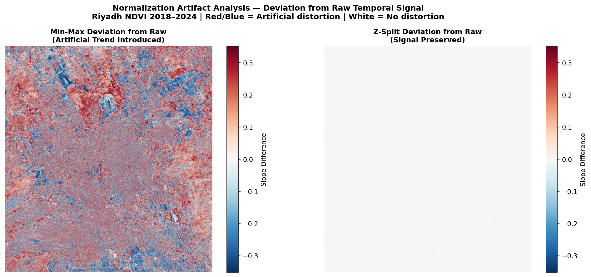
#### A. Normalization Artifact Analysis
|
|
164
|
+
|
|
165
|
+
The figure below shows the deviation of each normalization method from the raw temporal signal. Min-Max introduces large artificial trends across the entire scene (colored map). Z-Split introduces virtually no deviation (near-white map).
|
|
166
|
+
|
|
167
|
+
|
|
168
|
+
|
|
169
|
+
| Method | Mean Absolute Deviation | Std |
|
|
170
|
+
|--------|:-----------------------:|:---:|
|
|
171
|
+
| Min-Max | 0.1858 | 0.2091 |
|
|
172
|
+
| **Z-Split** | **0.0013** | **0.0017** |
|
|
173
|
+
|
|
174
|
+
Z-Split preserves the temporal signal with **143× greater fidelity** than Min-Max.
|
|
175
|
+
|
|
176
|
+
#### B. Linear Trend (Slope per pixel, 2018–2024)
|
|
146
177
|
|
|
147
178
|
| Method | Mean Slope | Std | Correlation with Raw |
|
|
148
179
|
|--------|:----------:|:---:|:--------------------:|
|
|
@@ -150,13 +181,11 @@ Validated on four Sentinel-2 NDVI scenes (March–April, 2018–2020–2022–20
|
|
|
150
181
|
| Min-Max | 0.027454 | 0.2170 | r = 0.511 |
|
|
151
182
|
| **Z-Split** | **−0.000120** | **0.0167** | **r = 0.995** |
|
|
152
183
|
|
|
153
|
-
|
|
184
|
+
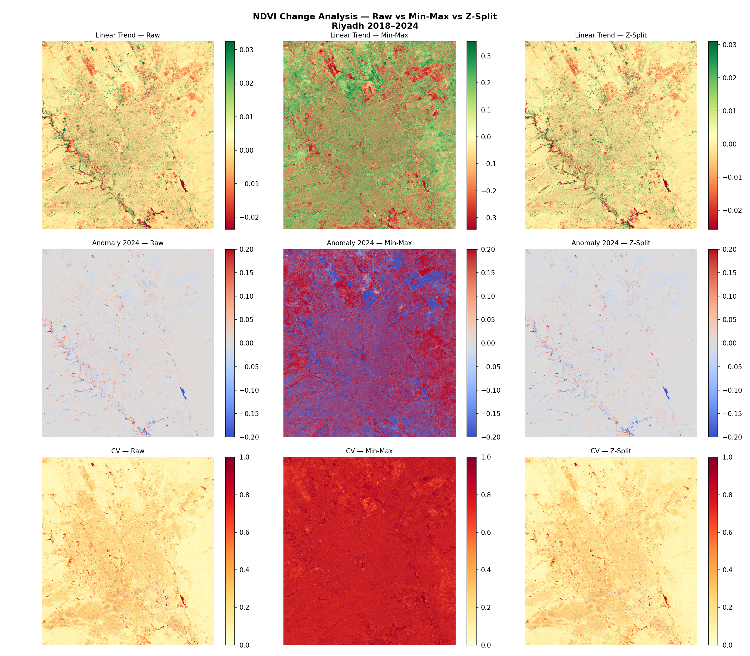
#### C. Multi-Temporal Change Maps
|
|
154
185
|
|
|
155
|
-
|
|
186
|
+
The figure below compares Linear Trend, Anomaly, and Coefficient of Variation maps across all three methods. Z-Split maps are visually and statistically consistent with raw data; Min-Max maps show spatially inverted anomaly patterns and 5.5× inflated variability.
|
|
156
187
|
|
|
157
|
-
|
|
158
|
-
|
|
159
|
-
#### C. Coefficient of Variation (CV across 2018–2024)
|
|
188
|
+
|
|
160
189
|
|
|
161
190
|
| Method | Mean CV |
|
|
162
191
|
|--------|:-------:|
|
|
@@ -164,14 +193,12 @@ Min-Max anomaly maps show spatially inverted patterns relative to raw data. Z-Sp
|
|
|
164
193
|
| **Z-Split** | **0.173** |
|
|
165
194
|
| Min-Max | 0.832 |
|
|
166
195
|
|
|
167
|
-
Min-Max inflates temporal variability by **5.5×**. Z-Split stays within 15% of the raw baseline.
|
|
168
|
-
|
|
169
196
|
#### D. Threshold Stability (Otsu across 11,424 patches)
|
|
170
197
|
|
|
171
198
|
| Method | Threshold Std |
|
|
172
199
|
|--------|:-------------:|
|
|
173
200
|
| Min-Max | 0.0882 |
|
|
174
|
-
|
|
|
201
|
+
| Z-Split | 0.2220 |
|
|
175
202
|
| Z-Score | 1.2012 |
|
|
176
203
|
|
|
177
204
|
> **Note:** For strongly unipolar NDVI in arid urban areas, Min-Max threshold stability is comparable to Z-Split. Z-Split's primary advantage is in bipolar indices with narrow near-zero distributions (NDWI, InSAR LOS), consistent with its design objective.
|
|
@@ -182,7 +209,7 @@ Min-Max inflates temporal variability by **5.5×**. Z-Split stays within 15% of
|
|
|
182
209
|
|
|
183
210
|
Most effective when:
|
|
184
211
|
- Values cluster near zero (NDWI in arid regions, InSAR LOS over stable terrain)
|
|
185
|
-
- Multi-temporal consistency is required
|
|
212
|
+
- Multi-temporal consistency is required (change detection, time series analysis)
|
|
186
213
|
- Otsu or zero-based thresholding is applied
|
|
187
214
|
- Cross-scene or cross-sensor comparisons are performed
|
|
188
215
|
|
|
@@ -199,14 +226,6 @@ Most effective when:
|
|
|
199
226
|
|
|
200
227
|
---
|
|
201
228
|
|
|
202
|
-
## Figures
|
|
203
|
-
|
|
204
|
-
**Figure 1:** Otsu threshold distribution across 11,424 spatial patches — Min-Max vs Z-Score vs Z-Split.
|
|
205
|
-
|
|
206
|
-
**Figure 2:** Multi-temporal NDVI change analysis (Linear Trend, Anomaly, CV) — Raw vs Min-Max vs Z-Split, Riyadh 2018–2024.
|
|
207
|
-
|
|
208
|
-
---
|
|
209
|
-
|
|
210
229
|
## Author
|
|
211
230
|
|
|
212
231
|
**Abdulrhman Almoadi**
|
|
@@ -1,6 +1,6 @@
|
|
|
1
1
|
# Z-Split Normalization (Zero-Preserving Split Normalization)
|
|
2
2
|
|
|
3
|
-
**Version:** 1.0.
|
|
3
|
+
**Version:** 1.0.1
|
|
4
4
|
**License:** MIT
|
|
5
5
|
|
|
6
6
|
---
|
|
@@ -74,6 +74,24 @@ result = normalize(your_bipolar_index)
|
|
|
74
74
|
|
|
75
75
|
---
|
|
76
76
|
|
|
77
|
+
## Practical Applications in Remote Sensing
|
|
78
|
+
|
|
79
|
+
Z-Split addresses a critical problem in any workflow involving bipolar indices across time or sensors:
|
|
80
|
+
|
|
81
|
+
**1. Change Detection**
|
|
82
|
+
Applying Min-Max before change detection introduces artificial trends that appear as land cover change but reflect only normalization artifacts. A report showing "15% vegetation decline" may be entirely attributable to normalization, not reality.
|
|
83
|
+
|
|
84
|
+
**2. Time Series Analysis**
|
|
85
|
+
Studies tracking floods, drought, or urban expansion over time require a clean temporal signal. Min-Max corrupts this signal by rescaling each scene independently to [0, 1], making year-to-year comparisons unreliable.
|
|
86
|
+
|
|
87
|
+
**3. Multi-temporal Machine Learning**
|
|
88
|
+
Models trained on Min-Max normalized multi-year data learn spurious patterns introduced by normalization rather than real spectral change. Z-Split ensures the training signal reflects actual surface conditions.
|
|
89
|
+
|
|
90
|
+
**4. InSAR and Displacement Monitoring**
|
|
91
|
+
In LOS displacement data, zero means no movement. Shifting zero through Min-Max misclassifies stable pixels as deforming, directly corrupting subsidence or uplift maps.
|
|
92
|
+
|
|
93
|
+
---
|
|
94
|
+
|
|
77
95
|
## Validation
|
|
78
96
|
|
|
79
97
|
### 1. NDWI — Optical Remote Sensing
|
|
@@ -84,7 +102,20 @@ Tested on Sentinel-2 NDWI data. Z-Split successfully expanded near-zero clustere
|
|
|
84
102
|
|
|
85
103
|
Validated on four Sentinel-2 NDVI scenes (March–April, 2018–2020–2022–2024) over Riyadh, Saudi Arabia (scale: 10 m, 5603 × 5129 pixels per scene) across 11,424 spatial patches.
|
|
86
104
|
|
|
87
|
-
#### A.
|
|
105
|
+
#### A. Normalization Artifact Analysis
|
|
106
|
+
|
|
107
|
+
The figure below shows the deviation of each normalization method from the raw temporal signal. Min-Max introduces large artificial trends across the entire scene (colored map). Z-Split introduces virtually no deviation (near-white map).
|
|
108
|
+
|
|
109
|
+

|
|
110
|
+
|
|
111
|
+
| Method | Mean Absolute Deviation | Std |
|
|
112
|
+
|--------|:-----------------------:|:---:|
|
|
113
|
+
| Min-Max | 0.1858 | 0.2091 |
|
|
114
|
+
| **Z-Split** | **0.0013** | **0.0017** |
|
|
115
|
+
|
|
116
|
+
Z-Split preserves the temporal signal with **143× greater fidelity** than Min-Max.
|
|
117
|
+
|
|
118
|
+
#### B. Linear Trend (Slope per pixel, 2018–2024)
|
|
88
119
|
|
|
89
120
|
| Method | Mean Slope | Std | Correlation with Raw |
|
|
90
121
|
|--------|:----------:|:---:|:--------------------:|
|
|
@@ -92,13 +123,11 @@ Validated on four Sentinel-2 NDVI scenes (March–April, 2018–2020–2022–20
|
|
|
92
123
|
| Min-Max | 0.027454 | 0.2170 | r = 0.511 |
|
|
93
124
|
| **Z-Split** | **−0.000120** | **0.0167** | **r = 0.995** |
|
|
94
125
|
|
|
95
|
-
|
|
126
|
+
#### C. Multi-Temporal Change Maps
|
|
96
127
|
|
|
97
|
-
|
|
128
|
+
The figure below compares Linear Trend, Anomaly, and Coefficient of Variation maps across all three methods. Z-Split maps are visually and statistically consistent with raw data; Min-Max maps show spatially inverted anomaly patterns and 5.5× inflated variability.
|
|
98
129
|
|
|
99
|
-
|
|
100
|
-
|
|
101
|
-
#### C. Coefficient of Variation (CV across 2018–2024)
|
|
130
|
+

|
|
102
131
|
|
|
103
132
|
| Method | Mean CV |
|
|
104
133
|
|--------|:-------:|
|
|
@@ -106,14 +135,12 @@ Min-Max anomaly maps show spatially inverted patterns relative to raw data. Z-Sp
|
|
|
106
135
|
| **Z-Split** | **0.173** |
|
|
107
136
|
| Min-Max | 0.832 |
|
|
108
137
|
|
|
109
|
-
Min-Max inflates temporal variability by **5.5×**. Z-Split stays within 15% of the raw baseline.
|
|
110
|
-
|
|
111
138
|
#### D. Threshold Stability (Otsu across 11,424 patches)
|
|
112
139
|
|
|
113
140
|
| Method | Threshold Std |
|
|
114
141
|
|--------|:-------------:|
|
|
115
142
|
| Min-Max | 0.0882 |
|
|
116
|
-
|
|
|
143
|
+
| Z-Split | 0.2220 |
|
|
117
144
|
| Z-Score | 1.2012 |
|
|
118
145
|
|
|
119
146
|
> **Note:** For strongly unipolar NDVI in arid urban areas, Min-Max threshold stability is comparable to Z-Split. Z-Split's primary advantage is in bipolar indices with narrow near-zero distributions (NDWI, InSAR LOS), consistent with its design objective.
|
|
@@ -124,7 +151,7 @@ Min-Max inflates temporal variability by **5.5×**. Z-Split stays within 15% of
|
|
|
124
151
|
|
|
125
152
|
Most effective when:
|
|
126
153
|
- Values cluster near zero (NDWI in arid regions, InSAR LOS over stable terrain)
|
|
127
|
-
- Multi-temporal consistency is required
|
|
154
|
+
- Multi-temporal consistency is required (change detection, time series analysis)
|
|
128
155
|
- Otsu or zero-based thresholding is applied
|
|
129
156
|
- Cross-scene or cross-sensor comparisons are performed
|
|
130
157
|
|
|
@@ -141,14 +168,6 @@ Most effective when:
|
|
|
141
168
|
|
|
142
169
|
---
|
|
143
170
|
|
|
144
|
-
## Figures
|
|
145
|
-
|
|
146
|
-
**Figure 1:** Otsu threshold distribution across 11,424 spatial patches — Min-Max vs Z-Score vs Z-Split.
|
|
147
|
-
|
|
148
|
-
**Figure 2:** Multi-temporal NDVI change analysis (Linear Trend, Anomaly, CV) — Raw vs Min-Max vs Z-Split, Riyadh 2018–2024.
|
|
149
|
-
|
|
150
|
-
---
|
|
151
|
-
|
|
152
171
|
## Author
|
|
153
172
|
|
|
154
173
|
**Abdulrhman Almoadi**
|
|
@@ -4,7 +4,7 @@ build-backend = "setuptools.build_meta"
|
|
|
4
4
|
|
|
5
5
|
[project]
|
|
6
6
|
name = "zsplit"
|
|
7
|
-
version = "1.0.
|
|
7
|
+
version = "1.0.2"
|
|
8
8
|
description = "Z-Split Normalization: Zero-Preserving Split Normalization for bipolar spectral indices"
|
|
9
9
|
readme = "README.md"
|
|
10
10
|
license = { file = "LICENSE" }
|
|
@@ -1,6 +1,6 @@
|
|
|
1
1
|
Metadata-Version: 2.4
|
|
2
2
|
Name: zsplit
|
|
3
|
-
Version: 1.0.
|
|
3
|
+
Version: 1.0.2
|
|
4
4
|
Summary: Z-Split Normalization: Zero-Preserving Split Normalization for bipolar spectral indices
|
|
5
5
|
Author-email: Abdulrhman Almoadi <aalmoadi@kacst.edu.sa>
|
|
6
6
|
License: MIT License
|
|
@@ -58,7 +58,7 @@ Dynamic: license-file
|
|
|
58
58
|
|
|
59
59
|
# Z-Split Normalization (Zero-Preserving Split Normalization)
|
|
60
60
|
|
|
61
|
-
**Version:** 1.0.
|
|
61
|
+
**Version:** 1.0.1
|
|
62
62
|
**License:** MIT
|
|
63
63
|
|
|
64
64
|
---
|
|
@@ -132,6 +132,24 @@ result = normalize(your_bipolar_index)
|
|
|
132
132
|
|
|
133
133
|
---
|
|
134
134
|
|
|
135
|
+
## Practical Applications in Remote Sensing
|
|
136
|
+
|
|
137
|
+
Z-Split addresses a critical problem in any workflow involving bipolar indices across time or sensors:
|
|
138
|
+
|
|
139
|
+
**1. Change Detection**
|
|
140
|
+
Applying Min-Max before change detection introduces artificial trends that appear as land cover change but reflect only normalization artifacts. A report showing "15% vegetation decline" may be entirely attributable to normalization, not reality.
|
|
141
|
+
|
|
142
|
+
**2. Time Series Analysis**
|
|
143
|
+
Studies tracking floods, drought, or urban expansion over time require a clean temporal signal. Min-Max corrupts this signal by rescaling each scene independently to [0, 1], making year-to-year comparisons unreliable.
|
|
144
|
+
|
|
145
|
+
**3. Multi-temporal Machine Learning**
|
|
146
|
+
Models trained on Min-Max normalized multi-year data learn spurious patterns introduced by normalization rather than real spectral change. Z-Split ensures the training signal reflects actual surface conditions.
|
|
147
|
+
|
|
148
|
+
**4. InSAR and Displacement Monitoring**
|
|
149
|
+
In LOS displacement data, zero means no movement. Shifting zero through Min-Max misclassifies stable pixels as deforming, directly corrupting subsidence or uplift maps.
|
|
150
|
+
|
|
151
|
+
---
|
|
152
|
+
|
|
135
153
|
## Validation
|
|
136
154
|
|
|
137
155
|
### 1. NDWI — Optical Remote Sensing
|
|
@@ -142,7 +160,20 @@ Tested on Sentinel-2 NDWI data. Z-Split successfully expanded near-zero clustere
|
|
|
142
160
|
|
|
143
161
|
Validated on four Sentinel-2 NDVI scenes (March–April, 2018–2020–2022–2024) over Riyadh, Saudi Arabia (scale: 10 m, 5603 × 5129 pixels per scene) across 11,424 spatial patches.
|
|
144
162
|
|
|
145
|
-
#### A.
|
|
163
|
+
#### A. Normalization Artifact Analysis
|
|
164
|
+
|
|
165
|
+
The figure below shows the deviation of each normalization method from the raw temporal signal. Min-Max introduces large artificial trends across the entire scene (colored map). Z-Split introduces virtually no deviation (near-white map).
|
|
166
|
+
|
|
167
|
+

|
|
168
|
+
|
|
169
|
+
| Method | Mean Absolute Deviation | Std |
|
|
170
|
+
|--------|:-----------------------:|:---:|
|
|
171
|
+
| Min-Max | 0.1858 | 0.2091 |
|
|
172
|
+
| **Z-Split** | **0.0013** | **0.0017** |
|
|
173
|
+
|
|
174
|
+
Z-Split preserves the temporal signal with **143× greater fidelity** than Min-Max.
|
|
175
|
+
|
|
176
|
+
#### B. Linear Trend (Slope per pixel, 2018–2024)
|
|
146
177
|
|
|
147
178
|
| Method | Mean Slope | Std | Correlation with Raw |
|
|
148
179
|
|--------|:----------:|:---:|:--------------------:|
|
|
@@ -150,13 +181,11 @@ Validated on four Sentinel-2 NDVI scenes (March–April, 2018–2020–2022–20
|
|
|
150
181
|
| Min-Max | 0.027454 | 0.2170 | r = 0.511 |
|
|
151
182
|
| **Z-Split** | **−0.000120** | **0.0167** | **r = 0.995** |
|
|
152
183
|
|
|
153
|
-
|
|
184
|
+
#### C. Multi-Temporal Change Maps
|
|
154
185
|
|
|
155
|
-
|
|
186
|
+
The figure below compares Linear Trend, Anomaly, and Coefficient of Variation maps across all three methods. Z-Split maps are visually and statistically consistent with raw data; Min-Max maps show spatially inverted anomaly patterns and 5.5× inflated variability.
|
|
156
187
|
|
|
157
|
-
|
|
158
|
-
|
|
159
|
-
#### C. Coefficient of Variation (CV across 2018–2024)
|
|
188
|
+

|
|
160
189
|
|
|
161
190
|
| Method | Mean CV |
|
|
162
191
|
|--------|:-------:|
|
|
@@ -164,14 +193,12 @@ Min-Max anomaly maps show spatially inverted patterns relative to raw data. Z-Sp
|
|
|
164
193
|
| **Z-Split** | **0.173** |
|
|
165
194
|
| Min-Max | 0.832 |
|
|
166
195
|
|
|
167
|
-
Min-Max inflates temporal variability by **5.5×**. Z-Split stays within 15% of the raw baseline.
|
|
168
|
-
|
|
169
196
|
#### D. Threshold Stability (Otsu across 11,424 patches)
|
|
170
197
|
|
|
171
198
|
| Method | Threshold Std |
|
|
172
199
|
|--------|:-------------:|
|
|
173
200
|
| Min-Max | 0.0882 |
|
|
174
|
-
|
|
|
201
|
+
| Z-Split | 0.2220 |
|
|
175
202
|
| Z-Score | 1.2012 |
|
|
176
203
|
|
|
177
204
|
> **Note:** For strongly unipolar NDVI in arid urban areas, Min-Max threshold stability is comparable to Z-Split. Z-Split's primary advantage is in bipolar indices with narrow near-zero distributions (NDWI, InSAR LOS), consistent with its design objective.
|
|
@@ -182,7 +209,7 @@ Min-Max inflates temporal variability by **5.5×**. Z-Split stays within 15% of
|
|
|
182
209
|
|
|
183
210
|
Most effective when:
|
|
184
211
|
- Values cluster near zero (NDWI in arid regions, InSAR LOS over stable terrain)
|
|
185
|
-
- Multi-temporal consistency is required
|
|
212
|
+
- Multi-temporal consistency is required (change detection, time series analysis)
|
|
186
213
|
- Otsu or zero-based thresholding is applied
|
|
187
214
|
- Cross-scene or cross-sensor comparisons are performed
|
|
188
215
|
|
|
@@ -199,14 +226,6 @@ Most effective when:
|
|
|
199
226
|
|
|
200
227
|
---
|
|
201
228
|
|
|
202
|
-
## Figures
|
|
203
|
-
|
|
204
|
-
**Figure 1:** Otsu threshold distribution across 11,424 spatial patches — Min-Max vs Z-Score vs Z-Split.
|
|
205
|
-
|
|
206
|
-
**Figure 2:** Multi-temporal NDVI change analysis (Linear Trend, Anomaly, CV) — Raw vs Min-Max vs Z-Split, Riyadh 2018–2024.
|
|
207
|
-
|
|
208
|
-
---
|
|
209
|
-
|
|
210
229
|
## Author
|
|
211
230
|
|
|
212
231
|
**Abdulrhman Almoadi**
|
|
File without changes
|
|
File without changes
|
|
File without changes
|
|
File without changes
|
|
File without changes
|
|
File without changes
|
|
File without changes
|
|
File without changes
|