wawi 0.0.5__tar.gz → 0.0.8__tar.gz
This diff represents the content of publicly available package versions that have been released to one of the supported registries. The information contained in this diff is provided for informational purposes only and reflects changes between package versions as they appear in their respective public registries.
Potentially problematic release.
This version of wawi might be problematic. Click here for more details.
- {wawi-0.0.5 → wawi-0.0.8}/PKG-INFO +61 -2
- wawi-0.0.8/README.md +100 -0
- {wawi-0.0.5 → wawi-0.0.8}/tests/test_IABSE_step11a.py +1 -3
- {wawi-0.0.5 → wawi-0.0.8}/tests/test_IABSE_step11c.py +1 -4
- {wawi-0.0.5 → wawi-0.0.8}/tests/test_IABSE_step2a.py +1 -3
- {wawi-0.0.5 → wawi-0.0.8}/wawi/__init__.py +1 -1
- {wawi-0.0.5 → wawi-0.0.8}/wawi/io.py +15 -15
- {wawi-0.0.5 → wawi-0.0.8}/wawi/modal.py +1 -1
- {wawi-0.0.5 → wawi-0.0.8}/wawi/plot.py +9 -6
- {wawi-0.0.5 → wawi-0.0.8}/wawi/wind.py +12 -19
- {wawi-0.0.5 → wawi-0.0.8}/wawi.egg-info/PKG-INFO +61 -2
- wawi-0.0.5/README.md +0 -41
- {wawi-0.0.5 → wawi-0.0.8}/LICENSE +0 -0
- {wawi-0.0.5 → wawi-0.0.8}/pyproject.toml +0 -0
- {wawi-0.0.5 → wawi-0.0.8}/setup.cfg +0 -0
- {wawi-0.0.5 → wawi-0.0.8}/tests/test_wind.py +0 -0
- {wawi-0.0.5 → wawi-0.0.8}/wawi/fe.py +0 -0
- {wawi-0.0.5 → wawi-0.0.8}/wawi/general.py +0 -0
- {wawi-0.0.5 → wawi-0.0.8}/wawi/identification.py +0 -0
- {wawi-0.0.5 → wawi-0.0.8}/wawi/prob.py +0 -0
- {wawi-0.0.5 → wawi-0.0.8}/wawi/random.py +0 -0
- {wawi-0.0.5 → wawi-0.0.8}/wawi/signal.py +0 -0
- {wawi-0.0.5 → wawi-0.0.8}/wawi/structural.py +0 -0
- {wawi-0.0.5 → wawi-0.0.8}/wawi/time_domain.py +0 -0
- {wawi-0.0.5 → wawi-0.0.8}/wawi/tools.py +0 -0
- {wawi-0.0.5 → wawi-0.0.8}/wawi/wave.py +0 -0
- {wawi-0.0.5 → wawi-0.0.8}/wawi/wind_code.py +0 -0
- {wawi-0.0.5 → wawi-0.0.8}/wawi.egg-info/SOURCES.txt +0 -0
- {wawi-0.0.5 → wawi-0.0.8}/wawi.egg-info/dependency_links.txt +0 -0
- {wawi-0.0.5 → wawi-0.0.8}/wawi.egg-info/requires.txt +0 -0
- {wawi-0.0.5 → wawi-0.0.8}/wawi.egg-info/top_level.txt +0 -0
|
@@ -1,6 +1,6 @@
|
|
|
1
1
|
Metadata-Version: 2.2
|
|
2
2
|
Name: wawi
|
|
3
|
-
Version: 0.0.
|
|
3
|
+
Version: 0.0.8
|
|
4
4
|
Summary: WAve and WInd response prediction
|
|
5
5
|
Author-email: "Knut A. Kvåle" <knut.a.kvale@ntnu.no>, Ole Øiseth <ole.oiseth@ntnu.no>, Aksel Fenerci <aksel.fenerci@ntnu.no>, Øivind Wiig Petersen <oyvind.w.petersen@ntnu.no>
|
|
6
6
|
License: MIT License
|
|
@@ -69,6 +69,65 @@ pip install git+https://www.github.com/knutankv/wawi.git@main
|
|
|
69
69
|
|
|
70
70
|
Quick start
|
|
71
71
|
=======================
|
|
72
|
+
Assuming a premade WAWI-model is created and saved as `MyModel.wwi´, it can be imported as follows:
|
|
73
|
+
|
|
74
|
+
```python
|
|
75
|
+
from wawi.model import Model, Windstate, Seastate
|
|
76
|
+
|
|
77
|
+
model = Model.load('MyModel.wwi')
|
|
78
|
+
model.n_modes = 50 # number of dry modes to use for computation
|
|
79
|
+
omega = np.arange(0.001, 2, 0.01) # frequency axis to use for FRF
|
|
80
|
+
```
|
|
81
|
+
|
|
82
|
+
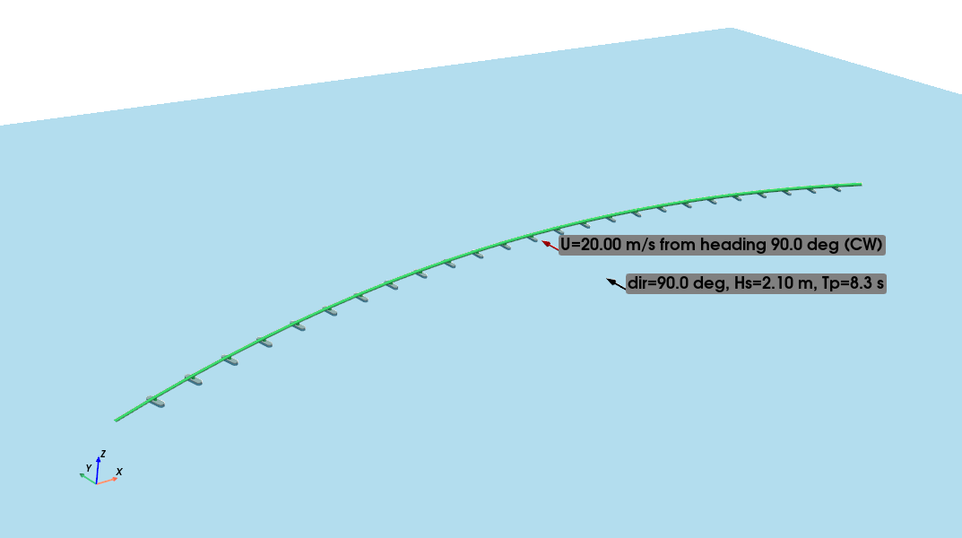
A windstate (U=20 m/s with origin 90 degrees and other required properties) and a seastate (Hs=2.1m, Tp=8.3s, gamma=8, s=12, heading 90 deg) is created and assigned to the model:
|
|
83
|
+
|
|
84
|
+
```python
|
|
85
|
+
# Wind state
|
|
86
|
+
U0 = 20.0
|
|
87
|
+
direction = 90.0
|
|
88
|
+
windstate = Windstate(U0, direction, Iu=0.136, Iw=0.072,
|
|
89
|
+
Au=6.8, Aw=9.4, Cuy=10.0, Cwy=6.5,
|
|
90
|
+
Lux=115, Lwx=9.58, spectrum_type='kaimal')
|
|
91
|
+
model.assign_windstate(windstate)
|
|
92
|
+
|
|
93
|
+
# Sea state
|
|
94
|
+
Hs = 2.1
|
|
95
|
+
Tp = 8.3
|
|
96
|
+
gamma = 8
|
|
97
|
+
s = 12
|
|
98
|
+
theta0 = 90.0
|
|
99
|
+
seastate = Seastate(Tp, Hs, gamma, theta0, s)
|
|
100
|
+
model.assign_seastate(seastate)
|
|
101
|
+
```
|
|
102
|
+
|
|
103
|
+
The model is plotted by envoking this command:
|
|
104
|
+
|
|
105
|
+
```python
|
|
106
|
+
model.plot()
|
|
107
|
+
```
|
|
108
|
+
|
|
109
|
+
which gives this plot of the model and the wind and wave states:
|
|
110
|
+
|
|
111
|
+
|
|
112
|
+
Then, response predictions can be run by the `run_freqsim` method or iterative modal analysis (combined system) conducted by `run_eig`:
|
|
113
|
+
|
|
114
|
+
```python
|
|
115
|
+
model.run_eig(include=['hydro', 'aero'])
|
|
116
|
+
model.run_freqsim(omega)
|
|
117
|
+
```
|
|
118
|
+
|
|
119
|
+
The results are stored in `model.results`, and consists of modal representation of the response (easily converted to relevant physical counterparts using built-in methods) or modal parameters of the combined system (natural frequencies, damping ratio, mode shapes).
|
|
120
|
+
|
|
121
|
+
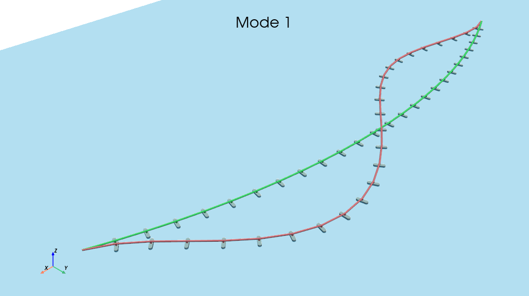
The resulting first mode shape is plotted as follows:
|
|
122
|
+
|
|
123
|
+
```python
|
|
124
|
+
model.plot_mode(0)
|
|
125
|
+
```
|
|
126
|
+
|
|
127
|
+
This results in this plot:
|
|
128
|
+
|
|
129
|
+
|
|
130
|
+
For more details and recommendations regarding the analysis setup, it is referred to the examples provided and the code reference.
|
|
72
131
|
|
|
73
132
|
Examples
|
|
74
133
|
=======================
|
|
@@ -79,7 +138,7 @@ References
|
|
|
79
138
|
|
|
80
139
|
Citation
|
|
81
140
|
=======================
|
|
82
|
-
Zenodo research entry:
|
|
141
|
+
Zenodo research entry: [](https://doi.org/10.5281/zenodo.14895014)
|
|
83
142
|
|
|
84
143
|
Support
|
|
85
144
|
=======================
|
wawi-0.0.8/README.md
ADDED
|
@@ -0,0 +1,100 @@
|
|
|
1
|
+

|
|
2
|
+
=======================
|
|
3
|
+
|
|
4
|
+
What is wawi?
|
|
5
|
+
=======================
|
|
6
|
+
WAWI is a Python toolbox for prediction of response of structures exposed to wind and wave excitation. The package is still under development in its alpha stage, and documentation and testing will be completed along the way.
|
|
7
|
+
|
|
8
|
+
|
|
9
|
+
Installation
|
|
10
|
+
========================
|
|
11
|
+
Either install via PyPI as follows:
|
|
12
|
+
|
|
13
|
+
```
|
|
14
|
+
pip install wawi
|
|
15
|
+
```
|
|
16
|
+
|
|
17
|
+
or install directly from github:
|
|
18
|
+
|
|
19
|
+
```
|
|
20
|
+
pip install git+https://www.github.com/knutankv/wawi.git@main
|
|
21
|
+
```
|
|
22
|
+
|
|
23
|
+
|
|
24
|
+
Quick start
|
|
25
|
+
=======================
|
|
26
|
+
Assuming a premade WAWI-model is created and saved as `MyModel.wwi´, it can be imported as follows:
|
|
27
|
+
|
|
28
|
+
```python
|
|
29
|
+
from wawi.model import Model, Windstate, Seastate
|
|
30
|
+
|
|
31
|
+
model = Model.load('MyModel.wwi')
|
|
32
|
+
model.n_modes = 50 # number of dry modes to use for computation
|
|
33
|
+
omega = np.arange(0.001, 2, 0.01) # frequency axis to use for FRF
|
|
34
|
+
```
|
|
35
|
+
|
|
36
|
+
A windstate (U=20 m/s with origin 90 degrees and other required properties) and a seastate (Hs=2.1m, Tp=8.3s, gamma=8, s=12, heading 90 deg) is created and assigned to the model:
|
|
37
|
+
|
|
38
|
+
```python
|
|
39
|
+
# Wind state
|
|
40
|
+
U0 = 20.0
|
|
41
|
+
direction = 90.0
|
|
42
|
+
windstate = Windstate(U0, direction, Iu=0.136, Iw=0.072,
|
|
43
|
+
Au=6.8, Aw=9.4, Cuy=10.0, Cwy=6.5,
|
|
44
|
+
Lux=115, Lwx=9.58, spectrum_type='kaimal')
|
|
45
|
+
model.assign_windstate(windstate)
|
|
46
|
+
|
|
47
|
+
# Sea state
|
|
48
|
+
Hs = 2.1
|
|
49
|
+
Tp = 8.3
|
|
50
|
+
gamma = 8
|
|
51
|
+
s = 12
|
|
52
|
+
theta0 = 90.0
|
|
53
|
+
seastate = Seastate(Tp, Hs, gamma, theta0, s)
|
|
54
|
+
model.assign_seastate(seastate)
|
|
55
|
+
```
|
|
56
|
+
|
|
57
|
+
The model is plotted by envoking this command:
|
|
58
|
+
|
|
59
|
+
```python
|
|
60
|
+
model.plot()
|
|
61
|
+
```
|
|
62
|
+
|
|
63
|
+
which gives this plot of the model and the wind and wave states:
|
|
64
|
+

|
|
65
|
+
|
|
66
|
+
Then, response predictions can be run by the `run_freqsim` method or iterative modal analysis (combined system) conducted by `run_eig`:
|
|
67
|
+
|
|
68
|
+
```python
|
|
69
|
+
model.run_eig(include=['hydro', 'aero'])
|
|
70
|
+
model.run_freqsim(omega)
|
|
71
|
+
```
|
|
72
|
+
|
|
73
|
+
The results are stored in `model.results`, and consists of modal representation of the response (easily converted to relevant physical counterparts using built-in methods) or modal parameters of the combined system (natural frequencies, damping ratio, mode shapes).
|
|
74
|
+
|
|
75
|
+
The resulting first mode shape is plotted as follows:
|
|
76
|
+
|
|
77
|
+
```python
|
|
78
|
+
model.plot_mode(0)
|
|
79
|
+
```
|
|
80
|
+
|
|
81
|
+
This results in this plot:
|
|
82
|
+

|
|
83
|
+
|
|
84
|
+
For more details and recommendations regarding the analysis setup, it is referred to the examples provided and the code reference.
|
|
85
|
+
|
|
86
|
+
Examples
|
|
87
|
+
=======================
|
|
88
|
+
Examples are provided as Jupyter Notebooks in the [examples folder](https://github.com/knutankv/wawi/tree/main/examples).
|
|
89
|
+
|
|
90
|
+
References
|
|
91
|
+
=======================
|
|
92
|
+
|
|
93
|
+
Citation
|
|
94
|
+
=======================
|
|
95
|
+
Zenodo research entry: [](https://doi.org/10.5281/zenodo.14895014)
|
|
96
|
+
|
|
97
|
+
Support
|
|
98
|
+
=======================
|
|
99
|
+
Please [open an issue](https://github.com/knutankv/wawi/issues/new) for support.
|
|
100
|
+
|
|
@@ -55,10 +55,7 @@ def iabse_11c_windstate(mean_v):
|
|
|
55
55
|
Cuz=0.0, Cwz=0.0,
|
|
56
56
|
Lux=200.0, Lwx=20.0,
|
|
57
57
|
x_ref=[0,0,0], rho=1.22,
|
|
58
|
-
|
|
59
|
-
'spectra_type': 'vonKarman'
|
|
60
|
-
}
|
|
61
|
-
)
|
|
58
|
+
spectrum_type='vonKarman')
|
|
62
59
|
return windstate
|
|
63
60
|
|
|
64
61
|
davenport = lambda fred: 2*(7*fred-1+np.exp(-7*fred))/(7*fred)**2
|
|
@@ -355,25 +355,25 @@ def import_wadam_hydro_transfer(wadam_file):
|
|
|
355
355
|
6-by-len(theta)-by-len(omega)
|
|
356
356
|
'''
|
|
357
357
|
|
|
358
|
-
string = ('.+W A V E P E R I O D.+=\s+(?P<period>.+):.+\n.+'
|
|
359
|
-
'H E A D I N G A N G L E.+=\s+(?P<theta>.+):(?:.*\n){5,10}'
|
|
358
|
+
string = (r'.+W A V E P E R I O D.+=\s+(?P<period>.+):.+\n.+'
|
|
359
|
+
r'H E A D I N G A N G L E.+=\s+(?P<theta>.+):(?:.*\n){5,10}'
|
|
360
360
|
|
|
361
|
-
'.+EXCITING FORCES AND MOMENTS FROM THE HASKIN RELATIONS(?:.*\n){4,6}\s+'
|
|
361
|
+
r'.+EXCITING FORCES AND MOMENTS FROM THE HASKIN RELATIONS(?:.*\n){4,6}\s+'
|
|
362
362
|
|
|
363
|
-
'-F1-\s+(?P<F1_real>[-?.E\d+]+)\s+(?P<F1_imag>[-?.E\d+]+)\s.+\n\s+'
|
|
364
|
-
'-F2-\s+(?P<F2_real>[-?.E\d+]+)\s+(?P<F2_imag>[-?.E\d+]+)\s.+\n\s+'
|
|
365
|
-
'-F3-\s+(?P<F3_real>[-?.E\d+]+)\s+(?P<F3_imag>[-?.E\d+]+)\s.+\n\s+'
|
|
366
|
-
'-F4-\s+(?P<F4_real>[-?.E\d+]+)\s+(?P<F4_imag>[-?.E\d+]+)\s.+\n\s+'
|
|
367
|
-
'-F5-\s+(?P<F5_real>[-?.E\d+]+)\s+(?P<F5_imag>[-?.E\d+]+)\s.+\n\s+'
|
|
368
|
-
'-F6-\s+(?P<F6_real>[-?.E\d+]+)\s+(?P<F6_imag>[-?.E\d+]+)\s.+\n')
|
|
363
|
+
r'-F1-\s+(?P<F1_real>[-?.E\d+]+)\s+(?P<F1_imag>[-?.E\d+]+)\s.+\n\s+'
|
|
364
|
+
r'-F2-\s+(?P<F2_real>[-?.E\d+]+)\s+(?P<F2_imag>[-?.E\d+]+)\s.+\n\s+'
|
|
365
|
+
r'-F3-\s+(?P<F3_real>[-?.E\d+]+)\s+(?P<F3_imag>[-?.E\d+]+)\s.+\n\s+'
|
|
366
|
+
r'-F4-\s+(?P<F4_real>[-?.E\d+]+)\s+(?P<F4_imag>[-?.E\d+]+)\s.+\n\s+'
|
|
367
|
+
r'-F5-\s+(?P<F5_real>[-?.E\d+]+)\s+(?P<F5_imag>[-?.E\d+]+)\s.+\n\s+'
|
|
368
|
+
r'-F6-\s+(?P<F6_real>[-?.E\d+]+)\s+(?P<F6_imag>[-?.E\d+]+)\s.+\n')
|
|
369
369
|
regex = re.compile(string)
|
|
370
370
|
|
|
371
|
-
nondim_string = ('\s+NON-DIMENSIONALIZING FACTORS:\n(?:.*\n)+'
|
|
372
|
-
'\s+RO\s+=\s+(?P<rho>[-?.E\d+]+)\n'
|
|
373
|
-
'\s+G\s+=\s+(?P<g>[-?.E\d+]+)\n'
|
|
374
|
-
'\s+VOL\s+=\s+(?P<vol>[-?.E\d+]+)\n'
|
|
375
|
-
'\s+L\s+=\s+(?P<l>[-?.E\d+]+)\n'
|
|
376
|
-
'\s+WA\s+=\s+(?P<wa>[-?.E\d+]+)')
|
|
371
|
+
nondim_string = (r'\s+NON-DIMENSIONALIZING FACTORS:\n(?:.*\n)+'
|
|
372
|
+
r'\s+RO\s+=\s+(?P<rho>[-?.E\d+]+)\n'
|
|
373
|
+
r'\s+G\s+=\s+(?P<g>[-?.E\d+]+)\n'
|
|
374
|
+
r'\s+VOL\s+=\s+(?P<vol>[-?.E\d+]+)\n'
|
|
375
|
+
r'\s+L\s+=\s+(?P<l>[-?.E\d+]+)\n'
|
|
376
|
+
r'\s+WA\s+=\s+(?P<wa>[-?.E\d+]+)')
|
|
377
377
|
|
|
378
378
|
regex_nondim = re.compile(nondim_string)
|
|
379
379
|
|
|
@@ -17,7 +17,7 @@ def maxreal(phi):
|
|
|
17
17
|
complex-valued modal transformation matrix, with vectors rotated to have maximum real parts
|
|
18
18
|
"""
|
|
19
19
|
|
|
20
|
-
angles = np.expand_dims(np.arange(0,np.pi
|
|
20
|
+
angles = np.expand_dims(np.arange(0,np.pi, 0.01), axis=0)
|
|
21
21
|
phi_max_real = np.zeros(np.shape(phi)).astype('complex')
|
|
22
22
|
for mode in range(0,np.shape(phi)[1]):
|
|
23
23
|
rot_mode = np.dot(np.expand_dims(phi[:, mode], axis=1), np.exp(angles*1j))
|
|
@@ -9,9 +9,9 @@ from scipy.interpolate import RectBivariateSpline, interp1d
|
|
|
9
9
|
|
|
10
10
|
def plot_ads(ad_dict, v, terms='stiffness', num=None, test_v=dict(), test_ad=dict(), zasso_type=False, ranges=None):
|
|
11
11
|
# v: v or K
|
|
12
|
-
if terms
|
|
12
|
+
if terms == 'stiffness':
|
|
13
13
|
terms = [['P4', 'P6', 'P3'], ['H6', 'H4', 'H3'], ['A6', 'A4', 'A3']]
|
|
14
|
-
elif terms
|
|
14
|
+
elif terms == 'damping':
|
|
15
15
|
terms = [['P1', 'P5', 'P2'], ['H5', 'H1', 'H2'], ['A5', 'A1', 'A2']]
|
|
16
16
|
|
|
17
17
|
# Create exponent defs for K_normalized plotting
|
|
@@ -60,9 +60,9 @@ def plot_ads(ad_dict, v, terms='stiffness', num=None, test_v=dict(), test_ad=dic
|
|
|
60
60
|
|
|
61
61
|
for col_ix in range(len(terms)):
|
|
62
62
|
if zasso_type:
|
|
63
|
-
ax[-1, col_ix].set_xlabel('$K$')
|
|
63
|
+
ax[-1, col_ix].set_xlabel(r'$K$')
|
|
64
64
|
else:
|
|
65
|
-
ax[-1, col_ix].set_xlabel('$V/(B\cdot \omega)$')
|
|
65
|
+
ax[-1, col_ix].set_xlabel(r'$V/(B\cdot \omega)$')
|
|
66
66
|
|
|
67
67
|
fig.tight_layout()
|
|
68
68
|
return fig, ax
|
|
@@ -98,7 +98,7 @@ def plot_dir_and_crests(theta0, Tp, arrow_length=100, origin=np.array([0,0]),
|
|
|
98
98
|
wave_length = 2*np.pi/get_kappa(2*np.pi/Tp, U=0.0)
|
|
99
99
|
|
|
100
100
|
plt.arrow(origin[0],origin[1], arrow_length*v[0], arrow_length*v[1], **arr_opts)
|
|
101
|
-
plt.text(origin[0], origin[1], f'$\\theta_0$ = {theta0}$^o$\n $T_p$={Tp} s\n
|
|
101
|
+
plt.text(origin[0], origin[1], f'$\\theta_0$ = {theta0}$^o$\n $T_p$={Tp} s\n $\\lambda=${wave_length:.0f} m')
|
|
102
102
|
|
|
103
103
|
dv = v*wave_length
|
|
104
104
|
for n in range(n_repeats):
|
|
@@ -317,7 +317,10 @@ def _set_axes_radius(ax, origin, radius):
|
|
|
317
317
|
ax.set_ylim3d([y - radius, y + radius])
|
|
318
318
|
ax.set_zlim3d([z - radius, z + radius])
|
|
319
319
|
|
|
320
|
-
def equal_3d(ax=
|
|
320
|
+
def equal_3d(ax=None):
|
|
321
|
+
if ax is None:
|
|
322
|
+
ax = plt.gca()
|
|
323
|
+
|
|
321
324
|
x_lims = np.array(ax.get_xlim())
|
|
322
325
|
y_lims = np.array(ax.get_ylim())
|
|
323
326
|
z_lims = np.array(ax.get_zlim())
|
|
@@ -526,7 +526,7 @@ def kaimal_auto(omega, Lx, A, sigma, V):
|
|
|
526
526
|
|
|
527
527
|
return S/(2*np.pi)
|
|
528
528
|
|
|
529
|
-
def
|
|
529
|
+
def von_karman_auto(omega, Lx, sigma, V):
|
|
530
530
|
|
|
531
531
|
A1 = [
|
|
532
532
|
0.0,
|
|
@@ -552,7 +552,7 @@ def von_Karman_auto(omega, Lx, sigma, V):
|
|
|
552
552
|
|
|
553
553
|
return S/(2*np.pi)
|
|
554
554
|
|
|
555
|
-
def generic_kaimal_matrix(omega, nodes, T_wind, A, sigma, C, Lx, U,
|
|
555
|
+
def generic_kaimal_matrix(omega, nodes, T_wind, A, sigma, C, Lx, U, spectrum_type='kaimal'):
|
|
556
556
|
# Adopted from MATLAB version. `nodes` is list with beef-nodes.
|
|
557
557
|
V = np.zeros(len(nodes)) # Initialize vector with mean wind in all nodes
|
|
558
558
|
Su = np.zeros([len(nodes), len(nodes)]) # One-point spectra for u component in all nodes
|
|
@@ -560,22 +560,16 @@ def generic_kaimal_matrix(omega, nodes, T_wind, A, sigma, C, Lx, U, options=None
|
|
|
560
560
|
Sw = np.zeros([len(nodes), len(nodes)]) # One-point spectra for w component in all nodes
|
|
561
561
|
xyz = np.zeros([len(nodes), 3]) # Nodes in wind coordinate system
|
|
562
562
|
|
|
563
|
-
if options is None:
|
|
564
|
-
options = {
|
|
565
|
-
'spectra_type': 'Kaimal'
|
|
566
|
-
}
|
|
567
|
-
|
|
568
563
|
for node_ix, node in enumerate(nodes):
|
|
569
564
|
xyz[node_ix,:] = (T_wind @ node.coordinates).T #Transform node coordinates to the wind coordinate system
|
|
570
565
|
V[node_ix] = U(node.coordinates) # Mean wind velocity in the nodes
|
|
571
566
|
|
|
572
|
-
if '
|
|
573
|
-
|
|
574
|
-
|
|
575
|
-
|
|
576
|
-
|
|
577
|
-
|
|
578
|
-
Su[node_ix,:], Sv[node_ix,:], Sw[node_ix,:] = kaimal_auto(omega, Lx, A, sigma, V[node_ix])
|
|
567
|
+
if 'karman' in spectrum_type.lower():
|
|
568
|
+
Su[node_ix,:], Sv[node_ix,:], Sw[node_ix,:] = von_karman_auto(omega, Lx, sigma, V[node_ix])
|
|
569
|
+
elif spectrum_type.lower() == 'kaimal':
|
|
570
|
+
Su[node_ix,:], Sv[node_ix,:], Sw[node_ix,:] = kaimal_auto(omega, Lx, A, sigma, V[node_ix]) # One point spectra for u component in all nodes
|
|
571
|
+
else:
|
|
572
|
+
raise ValueError('spectrum_type must either be defined as "vonKarman"/"Karman" or "Kaimal"')
|
|
579
573
|
|
|
580
574
|
x = xyz[:, 0]
|
|
581
575
|
y = xyz[:, 1]
|
|
@@ -822,7 +816,7 @@ def windaction_static(load_coefficients, elements, T_wind,
|
|
|
822
816
|
mean_wind = U(el.get_cog())
|
|
823
817
|
Vn = normal_wind(T_wind, el.T0)*mean_wind # Find the normal wind
|
|
824
818
|
BqBq = loadmatrix_fe_static(Vn, lc_fun(el), rho, B_fun(el), D_fun(el))
|
|
825
|
-
R1, R2 = loadvector(el.T0, BqBq, T_wind, el.L, static
|
|
819
|
+
R1, R2 = loadvector(el.T0, BqBq, T_wind, el.L, static=True) # Obtain the load vector for each element
|
|
826
820
|
|
|
827
821
|
RG[node1_dofs] = RG[node1_dofs] + R1[:,0] # Add the contribution from the element (end 1) to the system
|
|
828
822
|
RG[node2_dofs] = RG[node2_dofs] + R2[:,0] # Add the contribution from the element (end 2) to the system
|
|
@@ -833,12 +827,11 @@ def windaction_static(load_coefficients, elements, T_wind,
|
|
|
833
827
|
for node in nodes:
|
|
834
828
|
ix = node.index
|
|
835
829
|
n = np.r_[6*ix:6*ix+6]
|
|
836
|
-
RG_block[np.ix_(n)] = RG[n]
|
|
830
|
+
RG_block[np.ix_(n)] = RG[n]
|
|
837
831
|
|
|
838
|
-
|
|
839
|
-
genSqSq = phi.T @ RG_block
|
|
832
|
+
genF = phi.T @ RG_block
|
|
840
833
|
|
|
841
|
-
return
|
|
834
|
+
return genF
|
|
842
835
|
|
|
843
836
|
def K_from_ad(ad, V, w, B, rho):
|
|
844
837
|
if w==0:
|
|
@@ -1,6 +1,6 @@
|
|
|
1
1
|
Metadata-Version: 2.2
|
|
2
2
|
Name: wawi
|
|
3
|
-
Version: 0.0.
|
|
3
|
+
Version: 0.0.8
|
|
4
4
|
Summary: WAve and WInd response prediction
|
|
5
5
|
Author-email: "Knut A. Kvåle" <knut.a.kvale@ntnu.no>, Ole Øiseth <ole.oiseth@ntnu.no>, Aksel Fenerci <aksel.fenerci@ntnu.no>, Øivind Wiig Petersen <oyvind.w.petersen@ntnu.no>
|
|
6
6
|
License: MIT License
|
|
@@ -69,6 +69,65 @@ pip install git+https://www.github.com/knutankv/wawi.git@main
|
|
|
69
69
|
|
|
70
70
|
Quick start
|
|
71
71
|
=======================
|
|
72
|
+
Assuming a premade WAWI-model is created and saved as `MyModel.wwi´, it can be imported as follows:
|
|
73
|
+
|
|
74
|
+
```python
|
|
75
|
+
from wawi.model import Model, Windstate, Seastate
|
|
76
|
+
|
|
77
|
+
model = Model.load('MyModel.wwi')
|
|
78
|
+
model.n_modes = 50 # number of dry modes to use for computation
|
|
79
|
+
omega = np.arange(0.001, 2, 0.01) # frequency axis to use for FRF
|
|
80
|
+
```
|
|
81
|
+
|
|
82
|
+
A windstate (U=20 m/s with origin 90 degrees and other required properties) and a seastate (Hs=2.1m, Tp=8.3s, gamma=8, s=12, heading 90 deg) is created and assigned to the model:
|
|
83
|
+
|
|
84
|
+
```python
|
|
85
|
+
# Wind state
|
|
86
|
+
U0 = 20.0
|
|
87
|
+
direction = 90.0
|
|
88
|
+
windstate = Windstate(U0, direction, Iu=0.136, Iw=0.072,
|
|
89
|
+
Au=6.8, Aw=9.4, Cuy=10.0, Cwy=6.5,
|
|
90
|
+
Lux=115, Lwx=9.58, spectrum_type='kaimal')
|
|
91
|
+
model.assign_windstate(windstate)
|
|
92
|
+
|
|
93
|
+
# Sea state
|
|
94
|
+
Hs = 2.1
|
|
95
|
+
Tp = 8.3
|
|
96
|
+
gamma = 8
|
|
97
|
+
s = 12
|
|
98
|
+
theta0 = 90.0
|
|
99
|
+
seastate = Seastate(Tp, Hs, gamma, theta0, s)
|
|
100
|
+
model.assign_seastate(seastate)
|
|
101
|
+
```
|
|
102
|
+
|
|
103
|
+
The model is plotted by envoking this command:
|
|
104
|
+
|
|
105
|
+
```python
|
|
106
|
+
model.plot()
|
|
107
|
+
```
|
|
108
|
+
|
|
109
|
+
which gives this plot of the model and the wind and wave states:
|
|
110
|
+

|
|
111
|
+
|
|
112
|
+
Then, response predictions can be run by the `run_freqsim` method or iterative modal analysis (combined system) conducted by `run_eig`:
|
|
113
|
+
|
|
114
|
+
```python
|
|
115
|
+
model.run_eig(include=['hydro', 'aero'])
|
|
116
|
+
model.run_freqsim(omega)
|
|
117
|
+
```
|
|
118
|
+
|
|
119
|
+
The results are stored in `model.results`, and consists of modal representation of the response (easily converted to relevant physical counterparts using built-in methods) or modal parameters of the combined system (natural frequencies, damping ratio, mode shapes).
|
|
120
|
+
|
|
121
|
+
The resulting first mode shape is plotted as follows:
|
|
122
|
+
|
|
123
|
+
```python
|
|
124
|
+
model.plot_mode(0)
|
|
125
|
+
```
|
|
126
|
+
|
|
127
|
+
This results in this plot:
|
|
128
|
+

|
|
129
|
+
|
|
130
|
+
For more details and recommendations regarding the analysis setup, it is referred to the examples provided and the code reference.
|
|
72
131
|
|
|
73
132
|
Examples
|
|
74
133
|
=======================
|
|
@@ -79,7 +138,7 @@ References
|
|
|
79
138
|
|
|
80
139
|
Citation
|
|
81
140
|
=======================
|
|
82
|
-
Zenodo research entry:
|
|
141
|
+
Zenodo research entry: [](https://doi.org/10.5281/zenodo.14895014)
|
|
83
142
|
|
|
84
143
|
Support
|
|
85
144
|
=======================
|
wawi-0.0.5/README.md
DELETED
|
@@ -1,41 +0,0 @@
|
|
|
1
|
-

|
|
2
|
-
=======================
|
|
3
|
-
|
|
4
|
-
What is wawi?
|
|
5
|
-
=======================
|
|
6
|
-
WAWI is a Python toolbox for prediction of response of structures exposed to wind and wave excitation. The package is still under development in its alpha stage, and documentation and testing will be completed along the way.
|
|
7
|
-
|
|
8
|
-
|
|
9
|
-
Installation
|
|
10
|
-
========================
|
|
11
|
-
Either install via PyPI as follows:
|
|
12
|
-
|
|
13
|
-
```
|
|
14
|
-
pip install wawi
|
|
15
|
-
```
|
|
16
|
-
|
|
17
|
-
or install directly from github:
|
|
18
|
-
|
|
19
|
-
```
|
|
20
|
-
pip install git+https://www.github.com/knutankv/wawi.git@main
|
|
21
|
-
```
|
|
22
|
-
|
|
23
|
-
|
|
24
|
-
Quick start
|
|
25
|
-
=======================
|
|
26
|
-
|
|
27
|
-
Examples
|
|
28
|
-
=======================
|
|
29
|
-
Examples are provided as Jupyter Notebooks in the [examples folder](https://github.com/knutankv/wawi/tree/main/examples).
|
|
30
|
-
|
|
31
|
-
References
|
|
32
|
-
=======================
|
|
33
|
-
|
|
34
|
-
Citation
|
|
35
|
-
=======================
|
|
36
|
-
Zenodo research entry:
|
|
37
|
-
|
|
38
|
-
Support
|
|
39
|
-
=======================
|
|
40
|
-
Please [open an issue](https://github.com/knutankv/wawi/issues/new) for support.
|
|
41
|
-
|
|
File without changes
|
|
File without changes
|
|
File without changes
|
|
File without changes
|
|
File without changes
|
|
File without changes
|
|
File without changes
|
|
File without changes
|
|
File without changes
|
|
File without changes
|
|
File without changes
|
|
File without changes
|
|
File without changes
|
|
File without changes
|
|
File without changes
|
|
File without changes
|
|
File without changes
|
|
File without changes
|
|
File without changes
|