wawi 0.0.16__tar.gz → 0.0.18__tar.gz

{wawi-0.0.16 → wawi-0.0.18}/PKG-INFO

@@ -1,6 +1,6 @@
 Metadata-Version: 2.4
 Name: wawi
-Version: 0.0.16
+Version: 0.0.18
 Summary: WAve and WInd response prediction
 Author-email: "Knut A. Kvåle" <knut.a.kvale@ntnu.no>, Ole Øiseth <ole.oiseth@ntnu.no>, Aksel Fenerci <aksel.fenerci@ntnu.no>, Øivind Wiig Petersen <oyvind.w.petersen@ntnu.no>
 License: MIT License
@@ -92,17 +92,51 @@ pip install git+https://www.github.com/knutankv/wawi.git@main
 How does WAWI work?
 ======================
 By representing both aerodynamic and hydrodynamic motion-induced forces and excitation using a coordinate basis defined by the dry in-vacuum mode shapes of the structure, WAWI is able to versatily predict response based on input from any commercial FE software. The main structure used for response prediction is given in this figure:
+
 ![Model](https://raw.githubusercontent.com/knutankv/wawi/main/docs/flowchart.svg)
 
 The object structure of a WAWI model is given here:
-![Modelattributes](https://raw.githubusercontent.com/knutankv/wawi/main/docs/structure.svg)
+
+![Model attributes](https://raw.githubusercontent.com/knutankv/wawi/main/docs/structure.svg)
 
 Further details regarding hydrodynamic definitions initiated by the `Hydro` class is given below:
+
 ![Hydro](https://raw.githubusercontent.com/knutankv/wawi/main/docs/hydro_part.svg)
 
 Further details regarding aerodynamic definitions initiated by the `Aero` class is given below:
+
 ![Aero](https://raw.githubusercontent.com/knutankv/wawi/main/docs/aero_part.svg)
 
+Wave conditions
+----------------------
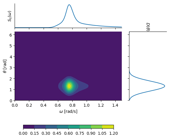
+The wave field definition is based on the assumption that the two-dimensional wave spectral density can be decomposed into a directional distribution and a one-dimensional wave spectral density, i.e.,  $S_\eta(\omega,\theta) = D(\theta) S(\omega)$. The two factors are defined using these well-known formulations:
+
+* $S(\omega)$: JONSWAP spectrum  (see [Hasselmann et al., 1973](https://pure.mpg.de/pubman/faces/ViewItemOverviewPage.jsp?itemId=item_3262854))
+* $D(\theta)$: cos-2s directional distribution (see Longuet-Higgins et al., 1963)
+
+Currents are defined by a homogeneous current speed `U` and corresponding direction `thetaU`.
+
+An example of a two-dimensional wave spectral density based on (arbitrarily chosen) parameters $H_s = 2.1$ m, $T_p = 2.1$ s, $\gamma = 4.0$, $s = 10$ and $\theta_0 = 75^\circ$ is shown in this plot:
+
+![2D wave PSD](https://raw.githubusercontent.com/knutankv/wawi/main/docs/wave_S2d.png)
+
+It is noted that you can easily assign custom functions of the `S` and `D` of the seastate (or customly on all pontoons for full control) instead of relying on the built in JONSWAP and cos-2s definitions.
+
+Wind conditions
+----------------------
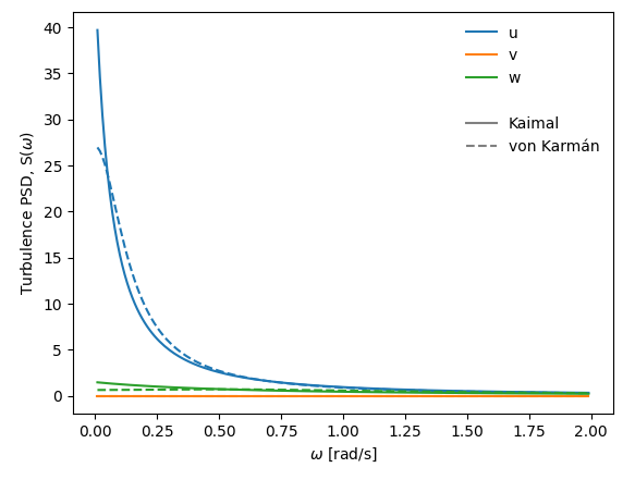
+The wind field is defined by single-point turbulence wind spectra (for all turbulence components $u$, $v$ and $w$) and coherence definitions.
+
+By default, wind spectra can be defined using these two definitions:
+
+* Kaimal spectrum defined by length scale parameters ($L^x_u$, $L^x_v$, $L^x_w$), spectral shape parameters ($A_u$, $A_v$ and $A_w$) and turbulence intensities ($I_u$, $I_v$ and $I_w$); see [Kaimal et al., 1972](https://www.climatexchange.nl/projects/alteddy/papers/Kaimal-1972.pdf)
+* von Karmán spectrum defined by only length scale parameters ($L^x_u$, $L^x_v$, $L^x_w$) and turbulence intensities ($I_u=\sigma_u/U$, $I_v=\sigma_v/U$ and $I_w=\sigma_w/U$); see [von Kármán, 1948](http://dx.doi.org/10.1073/pnas.34.11.530)
+
+Furthermore, the coherence of the wind field is defined by the nine decay parameters $C_{ux}$, $C_{vx}$, $C_{wx}$, $C_{uy}$, $C_{vy}$, $C_{wy}$, $C_{uz}$ $C_{vz}$, $C_{wz}$; see e.g. [Simiu and Scanlan, 1996](https://library.wur.nl/WebQuery/titel/1606468) for details.
+
+An example of turbulence spectral densities based on (arbitrarily chosen) parameters $I_u=0.136$, $I_v=0.0$, $I_w=0.072$, $L^x_u=115$, $L^x_w=9.58$, $A_u=6.8$ (only relevant for Kaimal-type) and $A_w=9.4$ (only relevant for Kaimal-type) is given below:
+
+![1D turbulence PSD](https://raw.githubusercontent.com/knutankv/wawi/main/docs/wind_psd.png)
+
 
 Quick start
 =======================
@@ -181,16 +215,20 @@ References
 =======================
 The following papers provide background for the implementation:
 
-* Beam (FE) description of aerodynamic forces: [Øiseth et al. (2012)](https://www.sciencedirect.com/science/article/abs/pii/S0168874X11001880)
 * Wave modelling and response prediction: [Kvåle et al. (2016)](https://www.sciencedirect.com/science/article/abs/pii/S004579491500334X)
 * Inhomogeneous wave modelling: [Kvåle et al. (2024)](https://www.sciencedirect.com/science/article/pii/S0141118723003437)
 * Hydrodynamic interaction effects: [Fenerci et al. (2022)](https://www.sciencedirect.com/science/article/pii/S095183392200017X)
+* Beam (FE) description of aerodynamic forces: [Øiseth et al. (2012)](https://www.sciencedirect.com/science/article/abs/pii/S0168874X11001880)
 * Wave-current interaction: [Fredriksen et al. (2024)](https://www.researchgate.net/profile/Arnt-Fredriksen/publication/386453916_On_the_wave-current_interaction_effect_on_linear_motion_for_floating_bridges/links/6751a40fabddbb448c65cbef/On-the-wave-current-interaction-effect-on-linear-motion-for-floating-bridges.pdf)
 
 
 Citation
 =======================
-Zenodo research entry: [![DOI](https://zenodo.org/badge/921621297.svg)](https://doi.org/10.5281/zenodo.14895014)
+Please cite the use of this software as follows:
+
+Kvåle, K. A., Fenerci, A., Petersen, Ø. W., & Øiseth, O. A. (2025). WAWI. Zenodo. https://doi.org/10.5281/zenodo.15482552
+[![DOI](https://zenodo.org/badge/921621297.svg)](https://doi.org/10.5281/zenodo.14895014)
+
 
 Support
 =======================

{wawi-0.0.16 → wawi-0.0.18}/README.md

@@ -45,17 +45,51 @@ pip install git+https://www.github.com/knutankv/wawi.git@main
 How does WAWI work?
 ======================
 By representing both aerodynamic and hydrodynamic motion-induced forces and excitation using a coordinate basis defined by the dry in-vacuum mode shapes of the structure, WAWI is able to versatily predict response based on input from any commercial FE software. The main structure used for response prediction is given in this figure:
+
 ![Model](https://raw.githubusercontent.com/knutankv/wawi/main/docs/flowchart.svg)
 
 The object structure of a WAWI model is given here:
-![Modelattributes](https://raw.githubusercontent.com/knutankv/wawi/main/docs/structure.svg)
+
+![Model attributes](https://raw.githubusercontent.com/knutankv/wawi/main/docs/structure.svg)
 
 Further details regarding hydrodynamic definitions initiated by the `Hydro` class is given below:
+
 ![Hydro](https://raw.githubusercontent.com/knutankv/wawi/main/docs/hydro_part.svg)
 
 Further details regarding aerodynamic definitions initiated by the `Aero` class is given below:
+
 ![Aero](https://raw.githubusercontent.com/knutankv/wawi/main/docs/aero_part.svg)
 
+Wave conditions
+----------------------
+The wave field definition is based on the assumption that the two-dimensional wave spectral density can be decomposed into a directional distribution and a one-dimensional wave spectral density, i.e.,  $S_\eta(\omega,\theta) = D(\theta) S(\omega)$. The two factors are defined using these well-known formulations:
+
+* $S(\omega)$: JONSWAP spectrum  (see [Hasselmann et al., 1973](https://pure.mpg.de/pubman/faces/ViewItemOverviewPage.jsp?itemId=item_3262854))
+* $D(\theta)$: cos-2s directional distribution (see Longuet-Higgins et al., 1963)
+
+Currents are defined by a homogeneous current speed `U` and corresponding direction `thetaU`.
+
+An example of a two-dimensional wave spectral density based on (arbitrarily chosen) parameters $H_s = 2.1$ m, $T_p = 2.1$ s, $\gamma = 4.0$, $s = 10$ and $\theta_0 = 75^\circ$ is shown in this plot:
+
+![2D wave PSD](https://raw.githubusercontent.com/knutankv/wawi/main/docs/wave_S2d.png)
+
+It is noted that you can easily assign custom functions of the `S` and `D` of the seastate (or customly on all pontoons for full control) instead of relying on the built in JONSWAP and cos-2s definitions.
+
+Wind conditions
+----------------------
+The wind field is defined by single-point turbulence wind spectra (for all turbulence components $u$, $v$ and $w$) and coherence definitions.
+
+By default, wind spectra can be defined using these two definitions:
+
+* Kaimal spectrum defined by length scale parameters ($L^x_u$, $L^x_v$, $L^x_w$), spectral shape parameters ($A_u$, $A_v$ and $A_w$) and turbulence intensities ($I_u$, $I_v$ and $I_w$); see [Kaimal et al., 1972](https://www.climatexchange.nl/projects/alteddy/papers/Kaimal-1972.pdf)
+* von Karmán spectrum defined by only length scale parameters ($L^x_u$, $L^x_v$, $L^x_w$) and turbulence intensities ($I_u=\sigma_u/U$, $I_v=\sigma_v/U$ and $I_w=\sigma_w/U$); see [von Kármán, 1948](http://dx.doi.org/10.1073/pnas.34.11.530)
+
+Furthermore, the coherence of the wind field is defined by the nine decay parameters $C_{ux}$, $C_{vx}$, $C_{wx}$, $C_{uy}$, $C_{vy}$, $C_{wy}$, $C_{uz}$ $C_{vz}$, $C_{wz}$; see e.g. [Simiu and Scanlan, 1996](https://library.wur.nl/WebQuery/titel/1606468) for details.
+
+An example of turbulence spectral densities based on (arbitrarily chosen) parameters $I_u=0.136$, $I_v=0.0$, $I_w=0.072$, $L^x_u=115$, $L^x_w=9.58$, $A_u=6.8$ (only relevant for Kaimal-type) and $A_w=9.4$ (only relevant for Kaimal-type) is given below:
+
+![1D turbulence PSD](https://raw.githubusercontent.com/knutankv/wawi/main/docs/wind_psd.png)
+
 
 Quick start
 =======================
@@ -134,16 +168,20 @@ References
 =======================
 The following papers provide background for the implementation:
 
-* Beam (FE) description of aerodynamic forces: [Øiseth et al. (2012)](https://www.sciencedirect.com/science/article/abs/pii/S0168874X11001880)
 * Wave modelling and response prediction: [Kvåle et al. (2016)](https://www.sciencedirect.com/science/article/abs/pii/S004579491500334X)
 * Inhomogeneous wave modelling: [Kvåle et al. (2024)](https://www.sciencedirect.com/science/article/pii/S0141118723003437)
 * Hydrodynamic interaction effects: [Fenerci et al. (2022)](https://www.sciencedirect.com/science/article/pii/S095183392200017X)
+* Beam (FE) description of aerodynamic forces: [Øiseth et al. (2012)](https://www.sciencedirect.com/science/article/abs/pii/S0168874X11001880)
 * Wave-current interaction: [Fredriksen et al. (2024)](https://www.researchgate.net/profile/Arnt-Fredriksen/publication/386453916_On_the_wave-current_interaction_effect_on_linear_motion_for_floating_bridges/links/6751a40fabddbb448c65cbef/On-the-wave-current-interaction-effect-on-linear-motion-for-floating-bridges.pdf)
 
 
 Citation
 =======================
-Zenodo research entry: [![DOI](https://zenodo.org/badge/921621297.svg)](https://doi.org/10.5281/zenodo.14895014)
+Please cite the use of this software as follows:
+
+Kvåle, K. A., Fenerci, A., Petersen, Ø. W., & Øiseth, O. A. (2025). WAWI. Zenodo. https://doi.org/10.5281/zenodo.15482552
+[![DOI](https://zenodo.org/badge/921621297.svg)](https://doi.org/10.5281/zenodo.14895014)
+
 
 Support
 =======================

{wawi-0.0.16 → wawi-0.0.18}/wawi/__init__.py

@@ -3,7 +3,7 @@
 '''
 __pdoc__ = {'wawi.ext.abq': False}
 
-__version__ = "0.0.16"
+__version__ = "0.0.18"
 
 # Other packages
 import numpy as np

wawi-0.0.18/wawi/fe.py

@@ -0,0 +1,381 @@
+# -*- coding: utf-8 -*-
+import numpy as np
+from .general import blkdiag, transform_unit
+
+'''
+FE-related tools.
+'''
+
+def intpoints_from_elements(nodes, elements, sort_axis=0):
+    """
+    Calculates the integration points (midpoints) for each element based on node coordinates.
+
+    Parameters
+    ----------
+    nodes : np.ndarray
+        Array of node coordinates with shape (n_nodes, 4), where columns represent node index and x, y, z coordinates.
+    elements : np.ndarray
+        Array of element connectivity with shape (n_elements, 2), where each row contains indices of the two nodes forming an element.
+    sort_axis : int, optional
+        Axis (0 for x, 1 for y, 2 for z) to sort the integration points by. Default is 0 (x-axis).
+
+    Returns
+    -------
+    x : np.ndarray
+        Array of x-coordinates of the integration points, sorted by the specified axis.
+    y : np.ndarray
+        Array of y-coordinates of the integration points, sorted by the specified axis.
+    z : np.ndarray
+        Array of z-coordinates of the integration points, sorted by the specified axis.
+
+    Notes
+    -----
+    Assumes that `nodeix_from_elements` is a function that returns the indices of the nodes for each element. Docstring is generated by Github Copilot.
+    """
+   
+    nodeix = nodeix_from_elements(elements, nodes).astype('int')
+
+    intpoints = (nodes[nodeix[:,0], 1:4]+nodes[nodeix[:,1], 1:4])/2
+    sortix = np.argsort(intpoints[:,sort_axis])
+    intpoints = intpoints[sortix, :]
+
+    x = intpoints[:, 0]
+    y = intpoints[:, 1]
+    z = intpoints[:, 2]
+
+    return x, y, z
+
+
+def nodeix_from_elements(element_matrix, node_matrix, return_as_flat=False):
+    """
+    Map element node labels to their corresponding indices in the node matrix.
+
+    Parameters
+    ----------
+    element_matrix : np.ndarray
+        Array of elements with shape (n_elements, m), where columns 1 and 2 contain node IDs for each element.
+    node_matrix : np.ndarray
+        Array of nodes with shape (n_nodes, k), where column 0 contains node IDs.
+    return_as_flat : bool, optional
+        If True, returns a 1D array of unique node indices used by all elements.
+        If False, returns a 2D array of shape (n_elements, 2) with node indices for each element.
+        Default is False.
+
+    Returns
+    -------
+    np.ndarray
+        If return_as_flat is False, returns a 2D array of node indices for each element (shape: n_elements, 2).
+        If return_as_flat is True, returns a 1D array of unique node indices.
+
+    Notes
+    -----
+    Each element is assumed to be defined by two node labels in columns 1 and 2 of element_matrix. Docstring is generated by GitHub Copilot.
+    """
+    nodeix = [None] * len(element_matrix[:, 0])
+    for element_ix, __ in enumerate(element_matrix[:, 0]):
+        node1 = element_matrix[element_ix, 1]
+        node2 = element_matrix[element_ix, 2]
+
+        nodeix1 = np.where(node_matrix[:, 0] == node1)[0][0]
+        nodeix2 = np.where(node_matrix[:, 0] == node2)[0][0]
+        nodeix[element_ix] = [nodeix1, nodeix2]
+
+    nodeix = np.array(nodeix)
+
+    if return_as_flat:
+        nodeix = np.unique(nodeix.flatten())
+
+    return nodeix
+
+
+def create_node_dict(element_dict, node_labels, x_nodes, y_nodes, z_nodes):
+    """
+    Creates a dictionary mapping element keys to their corresponding node data.
+
+    Parameters
+    ----------
+    element_dict : dict
+        A dictionary where each key corresponds to an element and each value contains information
+        about the nodes associated with that element.
+    node_labels : array-like
+        An array of node labels/IDs.
+    x_nodes : array-like
+        An array of x-coordinates for each node.
+    y_nodes : array-like
+        An array of y-coordinates for each node.
+    z_nodes : array-like
+        An array of z-coordinates for each node.
+
+    Returns
+    -------
+    node_dict : dict
+        A dictionary where each key matches an element key from `element_dict`, and each value is
+        an array containing the node label and coordinates (label, x, y, z) for the nodes
+        associated with that element.
+
+    Notes
+    -----
+    This function relies on the helper function `nodeix_from_elements` to determine the indices
+    of nodes associated with each element. Docstring is generated by GitHub Copilot.
+    """
+
+    node_dict = dict()
+    node_matrix = np.vstack([node_labels, x_nodes, y_nodes, z_nodes]).T
+
+    for key in element_dict.keys():
+        node_ix = nodeix_from_elements(element_dict[key], node_matrix, return_as_flat=True)
+        node_dict[key] = node_matrix[node_ix, :]
+
+    return node_dict
+
+
+def elements_with_node(element_matrix, node_label):
+    """
+    Finds elements containing a specific node and returns their labels, indices, and local node indices.
+    
+    Parameters
+    ----------
+    element_matrix : np.ndarray
+        A 2D array where each row represents an element. The first column contains element labels,
+        and the second and third columns contain node labels associated with each element.
+    node_label : int or float
+        The node label to search for within the element matrix.
+
+    Returns
+    -------
+    element_labels : np.ndarray
+        Array of element labels that contain the specified node.
+    element_ixs : np.ndarray
+        Array of indices in `element_matrix` where the specified node is found.
+    local_node_ix : np.ndarray
+        Array indicating the local node index (0 or 1) within each element where the node is found.
+
+    Examples
+    --------
+    >>> element_matrix = np.array([[1, 10, 20],
+    ...                            [2, 20, 30],
+    ...                            [3, 10, 30]])
+    >>> elements_with_node(element_matrix, 10)
+    (array([1, 3]), array([0, 2]), array([0., 0.]))
+
+    Notes
+    ---------
+    Docstring is generated by GitHub Copilot.
+    """
+    element_ixs1 = np.array(np.where(element_matrix[:,1]==node_label)).flatten()
+    element_ixs2 = np.array(np.where(element_matrix[:,2]==node_label)).flatten()
+
+    element_ixs = np.hstack([element_ixs1, element_ixs2])
+    element_labels = element_matrix[element_ixs, 0]
+
+    local_node_ix = np.zeros(np.shape(element_ixs))
+    local_node_ix[np.arange(0,len(element_ixs1))] = 0
+    local_node_ix[np.arange(len(element_ixs1), len(element_ixs1) + len(element_ixs2))] = 1
+
+    return element_labels, element_ixs, local_node_ix
+
+
+def nodes_to_beam_element_matrix(node_labels, first_element_label=1):
+    """
+    Generates an element connectivity matrix for beam elements from a sequence of node labels.
+
+    Parameters
+    ----------
+    node_labels : array_like
+        Sequence of node labels (integers or floats) defining the order of nodes along the beam.
+    first_element_label : int, optional
+        The label to assign to the first element. Default is 1.
+
+    Returns
+    -------
+    element_matrix : ndarray of shape (n_elements, 3)
+        Array where each row represents a beam element. The columns are:
+        [element_label, start_node_label, end_node_label].
+
+    Examples
+    --------
+    >>> nodes = [10, 20, 30, 40]
+    >>> nodes_to_beam_element_matrix(nodes)
+    array([[ 1., 10., 20.],
+           [ 2., 20., 30.],
+           [ 3., 30., 40.]])
+
+    Notes
+    ---------
+    Docstring is generated by GitHub Copilot.
+    """
+
+    n_nodes = len(node_labels)
+    n_elements = n_nodes-1
+    
+    element_matrix = np.empty([n_elements, 3])
+    element_matrix[:, 0] = np.arange(first_element_label,first_element_label+n_elements)
+    element_matrix[:, 1] = node_labels[0:-1]
+    element_matrix[:, 2] = node_labels[1:]
+
+    return element_matrix
+
+
+def node_ix_to_dof_ix(node_ix, n_dofs=6):
+    """
+    Converts a node index to a degree of freedom (DOF) index.
+    Each node has n_dofs degrees of freedom, and this function returns the corresponding DOF indices.
+
+    Parameters
+    ----------
+    node_ix : int
+        Index of the node for which to find the DOF indices.
+    n_dofs : int, optional
+        Number of degrees of freedom per node. Default is 6.
+    
+    Returns
+    -------
+    dof_ix : np.ndarray
+        Array of DOF indices corresponding to the given node index.
+
+    Examples
+    --------
+    >>> node_ix = 2
+    >>> n_dofs = 6
+    >>> dof_ix = node_ix_to_dof_ix(node_ix, n_dofs)
+    >>> print(dof_ix)
+    [12 13 14 15 16 17]
+
+    Notes
+    --------
+    Docstring is generated by GitHub Copilot.
+    
+    """
+    start = node_ix*n_dofs
+    stop = node_ix*n_dofs+n_dofs
+    dof_ix = []
+    for (i,j) in zip(start,stop):
+        dof_ix.append(np.arange(i,j))
+
+    dof_ix = np.array(dof_ix).flatten()
+
+    return dof_ix
+
+
+def dof_sel(arr, dof_sel, n_dofs=6, axis=0):
+    """
+    Selects degrees of freedom (DOFs) from an array along a specified axis.
+
+    Parameters
+    ----------
+    arr : np.ndarray
+        Input array from which to select DOFs.
+    dof_sel : array-like
+        Indices of the DOFs to select (relative to each block of n_dofs).
+    n_dofs : int, optional
+        Number of DOFs per node or block. Default is 6.
+    axis : int, optional
+        Axis along which to select DOFs. Default is 0.
+
+    Returns
+    -------
+    arr_sel : np.ndarray
+        Array containing only the selected DOFs along the specified axis.
+
+    Examples
+    --------
+    >>> arr = np.arange(18).reshape(3, 6)
+    >>> dof_sel(arr, [0, 2], n_dofs=6, axis=1)
+    array([[ 0,  2],
+           [ 6,  8],
+           [12, 14]])
+
+    Notes
+    -------
+    Docstring is generated by GitHub Copilot.
+    """
+
+    N = np.shape(arr)[axis]
+    all_ix = [range(dof_sel_i, N, n_dofs) for dof_sel_i in dof_sel]
+    sel_ix = np.array(all_ix).T.flatten()
+    
+    # Select the elements
+    arr_sel = np.take(arr, sel_ix, axis=axis)
+    
+    return arr_sel
+    
+
+
+def elements_from_common_nodes(element_matrix, selected_nodes):
+    """
+    Find elements that have both nodes in `selected_nodes`.
+
+    Parameters
+    ----------
+    element_matrix : np.ndarray
+        Array of elements with shape (n_elements, 3), where columns are [element_id, node1, node2].
+    selected_nodes : array-like
+        List or array of node labels to search for.
+
+    Returns
+    -------
+    selected_element_matrix : np.ndarray
+        Subset of `element_matrix` where both nodes are in `selected_nodes`.
+    sel_ix : np.ndarray
+        Indices of the selected elements in the original `element_matrix`.
+
+    Notes
+    -----
+    Only elements where both node1 and node2 are in `selected_nodes` are selected. Docstring is generated by GitHub Copilot.
+    """
+    
+    mask = np.isin(element_matrix[:, 1], selected_nodes) & np.isin(element_matrix[:, 2], selected_nodes)
+    sel_ix = np.where(mask)[0]
+    selected_element_matrix = element_matrix[sel_ix, :]
+
+    return selected_element_matrix, sel_ix
+
+
+def transform_elements(node_matrix, element_matrix, e2p, repeats=1):
+    """
+    Transforms elements from global to local coordinates.
+    Given a node matrix and an element matrix, this function computes the transformation matrices
+    from global to local coordinates for each element. The transformation is based on the direction
+    vector between the nodes of each element. The transformation matrices are constructed using
+    the `transform_unit` function and are repeated as specified.
+
+    Parameters
+    ----------
+    node_matrix : np.ndarray
+        Array of node data. The first column should contain node IDs, and the remaining columns
+        should contain node coordinates.
+    element_matrix : np.ndarray
+        Array of element data. Each row corresponds to an element, with the first column as the
+        element ID and the next columns as node IDs defining the element.
+    e2p : np.ndarray or similar
+        Additional parameter passed to `transform_unit` for transformation construction.
+    repeats : int, optional
+        Number of times to repeat the transformation block (default is 1).
+
+    Returns
+    -------
+    list of np.ndarray
+        List of transformation matrices, one for each element, mapping global to local coordinates.
+
+    Notes
+    -----
+    - Assumes that `transform_unit` and `blkdiag` functions are defined elsewhere.
+    - The function matches node IDs between `element_matrix` and `node_matrix` to determine node positions.
+    Docstring is generated by GitHub Copilot.
+    """
+
+    n_elements = np.shape(element_matrix)[0]
+    T_g2el = [None]*n_elements
+
+    for el in range(0, n_elements):
+        n1_ix = np.where(node_matrix[:,0]==element_matrix[el, 1])
+        n2_ix = np.where(node_matrix[:,0]==element_matrix[el, 2])
+
+        X1 = node_matrix[n1_ix, 1:]
+        X2 = node_matrix[n2_ix, 1:]
+        dx = X2-X1
+        e1 = dx/np.linalg.norm(dx)
+
+        T_g2el[el] = blkdiag(transform_unit(e1, e2p), repeats)   # Transform from global to local coordinates VLocal = T*VGlobal
+
+    return T_g2el