waveorder 2.2.0__tar.gz → 2.2.0rc0__tar.gz

{waveorder-2.2.0 → waveorder-2.2.0rc0}/.gitignore

@@ -150,4 +150,3 @@ recOrder/_version.py
 *.npz
 *.png
 *.tif[f]
-*.pdf

{waveorder-2.2.0 → waveorder-2.2.0rc0}/PKG-INFO

@@ -1,6 +1,6 @@
 Metadata-Version: 2.1
 Name: waveorder
-Version: 2.2.0
+Version: 2.2.0rc0
 Summary: Wave-optical simulations and deconvolution of optical properties
 Author-email: CZ Biohub SF <compmicro@czbiohub.org>
 Maintainer-email: Talon Chandler <talon.chandler@czbiohub.org>, Shalin Mehta <shalin.mehta@czbiohub.org>
@@ -53,99 +53,59 @@ Classifier: Operating System :: MacOS
 Requires-Python: >=3.10
 Description-Content-Type: text/markdown
 License-File: LICENSE
-Requires-Dist: numpy>=1.24
+Requires-Dist: numpy<2,>=1.21
 Requires-Dist: matplotlib>=3.1.1
 Requires-Dist: scipy>=1.3.0
 Requires-Dist: pywavelets>=1.1.1
 Requires-Dist: ipywidgets>=7.5.1
-Requires-Dist: torch>=2.4.1
+Requires-Dist: torch>=2.2.1
 Provides-Extra: dev
 Requires-Dist: pytest; extra == "dev"
 Requires-Dist: pytest-cov; extra == "dev"
-Provides-Extra: examples
-Requires-Dist: napari[all]; extra == "examples"
-Requires-Dist: jupyter; extra == "examples"
 
 # waveorder
 
-[![Python package index](https://img.shields.io/pypi/v/waveorder.svg)](https://pypi.org/project/waveorder)
-[![PyPI monthly downloads](https://img.shields.io/pypi/dm/waveorder.svg)](https://pypistats.org/packages/waveorder)
-[![Total downloads](https://pepy.tech/badge/waveorder)](https://pepy.tech/project/waveorder)
-[![GitHub contributors](https://img.shields.io/github/contributors-anon/mehta-lab/waveorder)](https://github.com/mehta-lab/waveorder/graphs/contributors)
-![GitHub Repo stars](https://img.shields.io/github/stars/mehta-lab/waveorder)
-![GitHub forks](https://img.shields.io/github/forks/mehta-lab/waveorder)
 ![PyPI - Python Version](https://img.shields.io/pypi/pyversions/waveorder)
-
+[![Downloads](https://pepy.tech/badge/waveorder)](https://pepy.tech/project/waveorder)
+[![Python package index](https://img.shields.io/pypi/v/waveorder.svg)](https://pypi.org/project/waveorder)
+[![Development Status](https://img.shields.io/pypi/status/napari.svg)](https://en.wikipedia.org/wiki/Software_release_life_cycle#Alpha)
 
 This computational imaging library enables wave-optical simulation and reconstruction of optical properties that report microscopic architectural order.
 
-## Computational label-agnostic imaging
+## Computational label-free imaging
 
-https://github.com/user-attachments/assets/4f9969e5-94ce-4e08-9f30-68314a905db6
+This vectorial wave simulator and reconstructor enabled the development of a new label-free imaging method, __permittivity tensor imaging (PTI)__, that measures density and  3D orientation of biomolecules with diffraction-limited resolution. These measurements are reconstructed from polarization-resolved images acquired with a sequence of oblique illuminations.
 
-`waveorder` enables simulations and reconstructions of label-agnostic microscopy data as described in the following [preprint](https://arxiv.org/abs/2412.09775)
-<details>	
-<summary> Chandler et al. 2024 </summary>
-<pre><code>
-@article{chandler_2024,
-    author = {Chandler, Talon and Hirata-Miyasaki, Eduardo and Ivanov, Ivan E. and Liu, Ziwen and Sundarraman, Deepika and Ryan, Allyson Quinn and Jacobo, Adrian and Balla, Keir and Mehta, Shalin B.},
-	title = {waveOrder: generalist framework for label-agnostic computational microscopy},
-	journal = {arXiv},
-	year = {2024},
-	month = dec,
-	eprint = {2412.09775},
-	doi = {10.48550/arXiv.2412.09775}
-}
-</code></pre>
-</details>
+The acquisition, calibration, background correction, reconstruction, and applications of PTI are described in the following [preprint](https://doi.org/10.1101/2020.12.15.422951):
 
-Specifically, `waveorder` enables simulation and reconstruction of 2D or 3D:
+```bibtex
+ L.-H. Yeh, I. E. Ivanov, B. B. Chhun, S.-M. Guo, E. Hashemi, J. R. Byrum, J. A. Pérez-Bermejo, H. Wang, Y. Yu, P. G. Kazansky, B. R. Conklin, M. H. Han, and S. B. Mehta, "uPTI: uniaxial permittivity tensor imaging of intrinsic density and anisotropy," bioRxiv 2020.12.15.422951 (2020).
+ ```
 
-1. __phase, projected retardance, and in-plane orientation__ from a polarization-diverse volumetric brightfield acquisition ([QLIPP](https://elifesciences.org/articles/55502)),
+In addition to PTI, `waveorder` enables simulations and reconstructions of subsets of label-free measurements with subsets of the acquired data:
 
-2. __phase__ from a volumetric brightfield acquisition ([2D phase](https://www.osapublishing.org/ao/abstract.cfm?uri=ao-54-28-8566)/[3D phase](https://www.osapublishing.org/ao/abstract.cfm?uri=ao-57-1-a205)),
+1. Reconstruction of 2D or 3D phase, projected retardance, and in-plane orientation from a polarization-diverse volumetric brightfield acquisition ([QLIPP](https://elifesciences.org/articles/55502))
 
-3. __phase__ from an illumination-diverse volumetric acquisition ([2D](https://www.osapublishing.org/oe/fulltext.cfm?uri=oe-23-9-11394&id=315599)/[3D](https://www.osapublishing.org/boe/fulltext.cfm?uri=boe-7-10-3940&id=349951) differential phase contrast),
+2. Reconstruction of 2D or 3D phase from a volumetric brightfield acquisition ([2D](https://www.osapublishing.org/ao/abstract.cfm?uri=ao-54-28-8566)/[3D (PODT)](https://www.osapublishing.org/ao/abstract.cfm?uri=ao-57-1-a205) phase)
 
-4. __fluorescence density__ from a widefield volumetric fluorescence acquisition (fluorescence deconvolution).  
+3. Reconstruction of 2D or 3D phase from an illumination-diverse volumetric acquisition ([2D](https://www.osapublishing.org/oe/fulltext.cfm?uri=oe-23-9-11394&id=315599)/[3D](https://www.osapublishing.org/boe/fulltext.cfm?uri=boe-7-10-3940&id=349951) differential phase contrast)
 
-The [examples](https://github.com/mehta-lab/waveorder/tree/main/examples) demonstrate simulations and reconstruction for 2D QLIPP, 3D PODT, 3D fluorescence deconvolution, and 2D/3D PTI methods.
-
-If you are interested in deploying QLIPP, phase from brightfield, or fluorescence deconvolution for label-agnostic imaging at scale, checkout our [napari plugin](https://www.napari-hub.org/plugins/recOrder-napari),  [`recOrder-napari`](https://github.com/mehta-lab/recOrder).
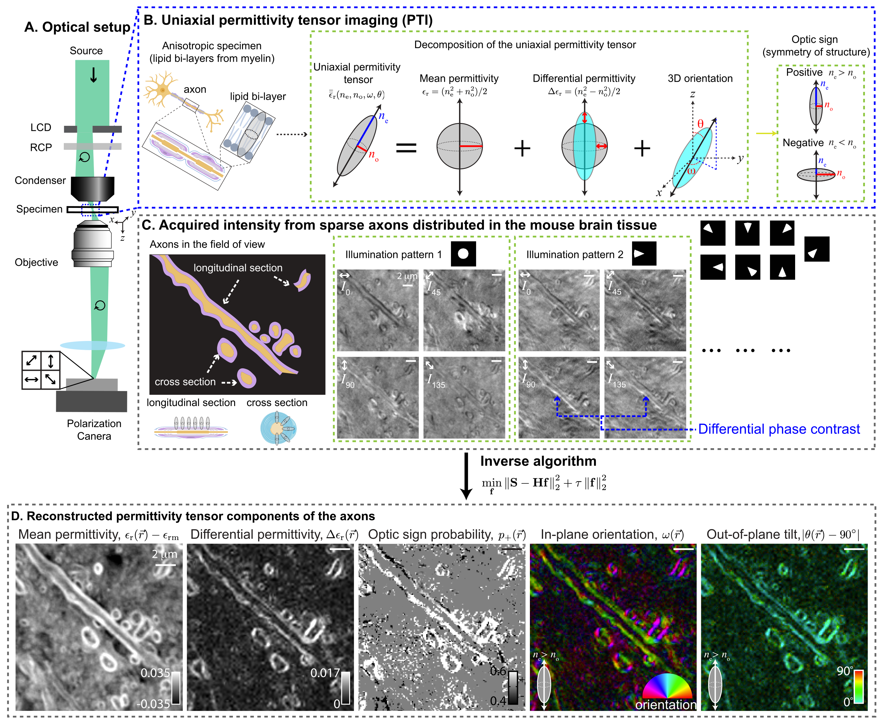
+PTI provides volumetric reconstructions of mean permittivity ($\propto$ material density), differential permittivity ($\propto$ material anisotropy), 3D orientation, and optic sign. The following figure summarizes PTI acquisition and reconstruction with a small optical section of the mouse brain tissue:
 
-## Permittivity tensor imaging 
+![Data_flow](https://github.com/mehta-lab/waveorder/blob/main/readme.png?raw=true)
 
-Additionally, `waveorder` enabled the development of a new label-free imaging method, __permittivity tensor imaging (PTI)__, that measures density and  3D orientation of biomolecules with diffraction-limited resolution. These measurements are reconstructed from polarization-resolved images acquired with a sequence of oblique illuminations.
 
-The acquisition, calibration, background correction, reconstruction, and applications of PTI are described in the following [paper](https://doi.org/10.1101/2020.12.15.422951) published in Nature Methods:
+The [examples](https://github.com/mehta-lab/waveorder/tree/main/examples) illustrate simulations and reconstruction for 2D QLIPP, 3D PODT, and 2D/3D PTI methods.
 
-<details>
-<summary> Yeh et al. 2024 </summary>
-<pre><code>
-@article{yeh_2024,
-	author = {Yeh, Li-Hao and Ivanov, Ivan E. and Chandler, Talon and Byrum, Janie R. and Chhun, Bryant B. and Guo, Syuan-Ming and Foltz, Cameron and Hashemi, Ezzat and Perez-Bermejo, Juan A. and Wang, Huijun and Yu, Yanhao and Kazansky, Peter G. and Conklin, Bruce R. and Han, May H. and Mehta, Shalin B.},
-	title = {Permittivity tensor imaging: modular label-free imaging of 3D dry mass and 3D orientation at high resolution},
-	journal = {Nature Methods},
-	volume = {21},
-	number = {7},
-	pages = {1257--1274},
-	year = {2024},
-	month = jul,
-	issn = {1548-7105},
-	publisher = {Nature Publishing Group},
-	doi = {10.1038/s41592-024-02291-w}
-}
-</code></pre>
-</details>
+If you are interested in deploying QLIPP or PODT for label-free imaging at scale, checkout our [napari plugin](https://www.napari-hub.org/plugins/recOrder-napari),  [`recOrder-napari`](https://github.com/mehta-lab/recOrder).
 
-PTI provides volumetric reconstructions of mean permittivity ($\propto$ material density), differential permittivity ($\propto$ material anisotropy), 3D orientation, and optic sign. The following figure summarizes PTI acquisition and reconstruction with a small optical section of the mouse brain tissue:
+## Correlative imaging
 
-![Data_flow](https://github.com/mehta-lab/waveorder/blob/main/readme.png?raw=true)
+In addition to label-free reconstruction algorithms, `waveorder` also implements widefield fluorescence and fluorescence polarization reconstruction algorithms for correlative label-free and fluorescence imaging.
 
-## Examples
-The [examples](https://github.com/mehta-lab/waveorder/tree/main/examples) illustrate simulations and reconstruction for 2D QLIPP, 3D phase from brightfield, and 2D/3D PTI methods.
+1. Correlative measurements of biomolecular density and orientation from polarization-diverse widefield imaging ([multimodal Instant PolScope](https://opg.optica.org/boe/fulltext.cfm?uri=boe-13-5-3102&id=472350))
 
-If you are interested in deploying QLIPP or phase from brightbrield, or fluorescence deconvolution for label-agnostic imaging at scale, checkout our [napari plugin](https://www.napari-hub.org/plugins/recOrder-napari),  [`recOrder-napari`](https://github.com/mehta-lab/recOrder).
+We provide an [example notebook](https://github.com/mehta-lab/waveorder/blob/main/examples/documentation/fluorescence_deconvolution/fluorescence_deconv.ipynb) for widefield fluorescence deconvolution.
 
 ## Citation
 
@@ -153,10 +113,10 @@ Please cite this repository, along with the relevant preprint or paper, if you u
 
 ## Installation
 
-Create a virtual environment:
+(Optional but recommended) install [anaconda](https://www.anaconda.com/products/distribution) and create a virtual environment:
 
 ```sh
-conda create -y -n waveorder python=3.10
+conda create -y -n waveorder python=3.11
 conda activate waveorder
 ```
 
@@ -173,11 +133,12 @@ python
 >>> import waveorder
 ```
 
-(Optional) Install example dependencies, clone the repository, and run an example script:
+(Optional) Download the repository, install `jupyter`, and experiment with the example notebooks
+
 ```sh
-pip install waveorder[examples]
 git clone https://github.com/mehta-lab/waveorder.git
-python waveorder/examples/models/phase_thick_3d.py
+pip install jupyter
+jupyter notebook ./waveorder/examples/
 ```
 
 (M1 users) `pytorch` has [incomplete GPU support](https://github.com/pytorch/pytorch/issues/77764),

waveorder-2.2.0rc0/README.md

@@ -0,0 +1,82 @@
+# waveorder
+
+![PyPI - Python Version](https://img.shields.io/pypi/pyversions/waveorder)
+[![Downloads](https://pepy.tech/badge/waveorder)](https://pepy.tech/project/waveorder)
+[![Python package index](https://img.shields.io/pypi/v/waveorder.svg)](https://pypi.org/project/waveorder)
+[![Development Status](https://img.shields.io/pypi/status/napari.svg)](https://en.wikipedia.org/wiki/Software_release_life_cycle#Alpha)
+
+This computational imaging library enables wave-optical simulation and reconstruction of optical properties that report microscopic architectural order.
+
+## Computational label-free imaging
+
+This vectorial wave simulator and reconstructor enabled the development of a new label-free imaging method, __permittivity tensor imaging (PTI)__, that measures density and  3D orientation of biomolecules with diffraction-limited resolution. These measurements are reconstructed from polarization-resolved images acquired with a sequence of oblique illuminations.
+
+The acquisition, calibration, background correction, reconstruction, and applications of PTI are described in the following [preprint](https://doi.org/10.1101/2020.12.15.422951):
+
+```bibtex
+ L.-H. Yeh, I. E. Ivanov, B. B. Chhun, S.-M. Guo, E. Hashemi, J. R. Byrum, J. A. Pérez-Bermejo, H. Wang, Y. Yu, P. G. Kazansky, B. R. Conklin, M. H. Han, and S. B. Mehta, "uPTI: uniaxial permittivity tensor imaging of intrinsic density and anisotropy," bioRxiv 2020.12.15.422951 (2020).
+ ```
+
+In addition to PTI, `waveorder` enables simulations and reconstructions of subsets of label-free measurements with subsets of the acquired data:
+
+1. Reconstruction of 2D or 3D phase, projected retardance, and in-plane orientation from a polarization-diverse volumetric brightfield acquisition ([QLIPP](https://elifesciences.org/articles/55502))
+
+2. Reconstruction of 2D or 3D phase from a volumetric brightfield acquisition ([2D](https://www.osapublishing.org/ao/abstract.cfm?uri=ao-54-28-8566)/[3D (PODT)](https://www.osapublishing.org/ao/abstract.cfm?uri=ao-57-1-a205) phase)
+
+3. Reconstruction of 2D or 3D phase from an illumination-diverse volumetric acquisition ([2D](https://www.osapublishing.org/oe/fulltext.cfm?uri=oe-23-9-11394&id=315599)/[3D](https://www.osapublishing.org/boe/fulltext.cfm?uri=boe-7-10-3940&id=349951) differential phase contrast)
+
+PTI provides volumetric reconstructions of mean permittivity ($\propto$ material density), differential permittivity ($\propto$ material anisotropy), 3D orientation, and optic sign. The following figure summarizes PTI acquisition and reconstruction with a small optical section of the mouse brain tissue:
+
+![Data_flow](https://github.com/mehta-lab/waveorder/blob/main/readme.png?raw=true)
+
+
+The [examples](https://github.com/mehta-lab/waveorder/tree/main/examples) illustrate simulations and reconstruction for 2D QLIPP, 3D PODT, and 2D/3D PTI methods.
+
+If you are interested in deploying QLIPP or PODT for label-free imaging at scale, checkout our [napari plugin](https://www.napari-hub.org/plugins/recOrder-napari),  [`recOrder-napari`](https://github.com/mehta-lab/recOrder).
+
+## Correlative imaging
+
+In addition to label-free reconstruction algorithms, `waveorder` also implements widefield fluorescence and fluorescence polarization reconstruction algorithms for correlative label-free and fluorescence imaging.
+
+1. Correlative measurements of biomolecular density and orientation from polarization-diverse widefield imaging ([multimodal Instant PolScope](https://opg.optica.org/boe/fulltext.cfm?uri=boe-13-5-3102&id=472350))
+
+We provide an [example notebook](https://github.com/mehta-lab/waveorder/blob/main/examples/documentation/fluorescence_deconvolution/fluorescence_deconv.ipynb) for widefield fluorescence deconvolution.
+
+## Citation
+
+Please cite this repository, along with the relevant preprint or paper, if you use or adapt this code. The citation information can be found by clicking "Cite this repository" button in the About section in the right sidebar.
+
+## Installation
+
+(Optional but recommended) install [anaconda](https://www.anaconda.com/products/distribution) and create a virtual environment:
+
+```sh
+conda create -y -n waveorder python=3.11
+conda activate waveorder
+```
+
+Install `waveorder` from PyPI:
+
+```sh
+pip install waveorder
+```
+
+Use `waveorder` in your scripts:
+
+```sh
+python
+>>> import waveorder
+```
+
+(Optional) Download the repository, install `jupyter`, and experiment with the example notebooks
+
+```sh
+git clone https://github.com/mehta-lab/waveorder.git
+pip install jupyter
+jupyter notebook ./waveorder/examples/
+```
+
+(M1 users) `pytorch` has [incomplete GPU support](https://github.com/pytorch/pytorch/issues/77764),
+so please use `export PYTORCH_ENABLE_MPS_FALLBACK=1`
+to allow some operators to fallback to CPU
+if you plan to use GPU acceleration for polarization reconstruction. 

waveorder-2.2.0rc0/examples/README.md

@@ -0,0 +1,7 @@
+`waveorder` is undergoing a significant refactor, and this `examples/` folder serves as a good place to understand the current state of the repository.
+
+The `models/` folder demonstrates the latest functionality of `waveorder`. These scripts will run as is in an environment with `waveorder` and `napari` installed. Each script demonstrates a simulation and reconstruction with a **model**: a specific set of assumptions about the sample and the data being acquired. 
+
+The `maintenance/` folder demonstrates the functionality of `waveorder` that we plan to move to `models/`. These scripts can be run as is, and they are being maintained with tests.
+
+The `documentation/` folder consists of examples that demonstrate reconstruction with real data. These examples require access to the complete datasets, so they are not being actively maintained and serve primarily as documentation.

{waveorder-2.2.0 → waveorder-2.2.0rc0}/examples/documentation/PTI_experiment/PTI_Experiment_Recon3D_anisotropic_target_small.py

@@ -6,12 +6,11 @@ import matplotlib.pyplot as plt
 from numpy.fft import fftshift
 
 import waveorder as wo
-from waveorder import optics, waveorder_reconstructor, util
+from waveorder import optics, waveorder_reconstructor, util, visual
 
 import zarr
 from pathlib import Path
 from iohub import open_ome_zarr
-from waveorder.visuals import jupyter_visuals
 
 # %%
 # Initialization
@@ -111,7 +110,7 @@ for i in range(len(Source)):
     Source_PolState[i, 1] = E_in[1]
 
 
-jupyter_visuals.plot_multicolumn(
+visual.plot_multicolumn(
     fftshift(Source, axes=(1, 2)), origin="lower", num_col=5
 )
 
@@ -163,7 +162,7 @@ S_image_tm[2] = (
 
 # %%
 # browse raw intensity stacks (stack_idx_1: z index, stack_idx2: pattern index)
-jupyter_visuals.parallel_5D_viewer(
+visual.parallel_5D_viewer(
     np.transpose(I_meas[:, :, :, :, ::-1], (4, 1, 0, 2, 3)),
     num_col=4,
     size=10,
@@ -172,7 +171,7 @@ jupyter_visuals.parallel_5D_viewer(
 
 # %%
 # browse uncorrected Stokes parameters (stack_idx_1: z index, stack_idx2: pattern index)
-jupyter_visuals.parallel_5D_viewer(
+visual.parallel_5D_viewer(
     np.transpose(S_image_recon, (4, 1, 0, 2, 3)),
     num_col=3,
     size=8,
@@ -183,7 +182,7 @@ jupyter_visuals.parallel_5D_viewer(
 
 # %%
 # browse corrected Stokes parameters (stack_idx_1: z index, stack_idx2: pattern index)
-jupyter_visuals.parallel_5D_viewer(
+visual.parallel_5D_viewer(
     np.transpose(S_image_tm, (4, 1, 0, 2, 3)),
     num_col=3,
     size=8,
@@ -214,7 +213,7 @@ f_tensor = setup.scattering_potential_tensor_recon_3D_vec(
 
 # %%
 # browse the z-stack of components of scattering potential tensor
-jupyter_visuals.parallel_4D_viewer(
+visual.parallel_4D_viewer(
     np.transpose(f_tensor, (3, 0, 1, 2)),
     num_col=4,
     origin="lower",
@@ -279,7 +278,7 @@ differential_permittivity_PT = np.array(
 
 # %%
 # browse the reconstructed physical properties
-jupyter_visuals.parallel_4D_viewer(
+visual.parallel_4D_viewer(
     np.transpose(
         np.stack(
             [
@@ -547,7 +546,7 @@ ax[5, 1].set_title("inclination (+) (xz)")
 
 # %%
 # browse XY planes of the phase and differential permittivity
-jupyter_visuals.parallel_4D_viewer(
+visual.parallel_4D_viewer(
     np.transpose(
         [
             np.clip(phase_PT, phase_min, phase_max),
@@ -586,7 +585,7 @@ orientation_3D_image = np.transpose(
     ),
     (3, 1, 2, 0),
 )
-orientation_3D_image_RGB = jupyter_visuals.orientation_3D_to_rgb(
+orientation_3D_image_RGB = visual.orientation_3D_to_rgb(
     orientation_3D_image, interp_belt=20 / 180 * np.pi, sat_factor=1
 )
 
@@ -601,7 +600,7 @@ plt.imshow(
 
 # plot the top view of 3D orientation colorsphere
 plt.figure(figsize=(3, 3))
-jupyter_visuals.orientation_3D_colorwheel(
+visual.orientation_3D_colorwheel(
     wheelsize=256, circ_size=50, interp_belt=20 / 180 * np.pi, sat_factor=1
 )
 
@@ -640,7 +639,7 @@ plt.imshow(
     in_plane_orientation[:, y_layer], origin="lower", aspect=z_step / ps
 )
 plt.figure(figsize=(3, 3))
-jupyter_visuals.orientation_2D_colorwheel()
+visual.orientation_2D_colorwheel()
 
 # %%
 # out-of-plane tilt
@@ -687,7 +686,7 @@ z_layer = 44
 
 fig, ax = plt.subplots(1, 1, figsize=(15, 15))
 
-jupyter_visuals.plot3DVectorField(
+visual.plot3DVectorField(
     np.abs(differential_permittivity_PT[1, :, :, z_layer]),
     azimuth[1, :, :, z_layer],
     theta[1, :, :, z_layer],
@@ -723,7 +722,7 @@ plt.imshow(
 # %%
 # Angular histogram of 3D orientation
 
-jupyter_visuals.orientation_3D_hist(
+visual.orientation_3D_hist(
     azimuth[1].flatten(),
     theta[1].flatten(),
     ret_mask.flatten(),

{waveorder-2.2.0 → waveorder-2.2.0rc0}/examples/maintenance/PTI_simulation/PTI_Simulation_Forward_2D3D.py

@@ -15,9 +15,9 @@ from numpy.fft import fftshift
 from waveorder import (
     optics,
     waveorder_simulator,
+    visual,
     util,
 )
-from waveorder.visuals import jupyter_visuals
 
 #####################################################################
 # Initialization - imaging system and sample                        #
@@ -145,7 +145,7 @@ biref_map = ne_map_copy - no_map_copy
 ### Visualize sample properties
 
 #### XY sections
-jupyter_visuals.plot_multicolumn(
+visual.plot_multicolumn(
     [
         target[:, :, z_layer],
         azimuth[:, :, z_layer] % (2 * np.pi),
@@ -158,7 +158,7 @@ jupyter_visuals.plot_multicolumn(
     set_title=True,
 )
 #### XZ sections
-jupyter_visuals.plot_multicolumn(
+visual.plot_multicolumn(
     [
         np.transpose(target[y_layer, :, :]),
         np.transpose(azimuth[y_layer, :, :]) % (2 * np.pi),
@@ -197,7 +197,7 @@ orientation_3D_image = np.transpose(
     ),
     (3, 1, 2, 0),
 )
-orientation_3D_image_RGB = jupyter_visuals.orientation_3D_to_rgb(
+orientation_3D_image_RGB = visual.orientation_3D_to_rgb(
     orientation_3D_image, interp_belt=20 / 180 * np.pi, sat_factor=1
 )
 
@@ -206,7 +206,7 @@ plt.imshow(orientation_3D_image_RGB[z_layer], origin="lower")
 plt.figure(figsize=(10, 10))
 plt.imshow(orientation_3D_image_RGB[:, y_layer], origin="lower")
 plt.figure(figsize=(3, 3))
-jupyter_visuals.orientation_3D_colorwheel(
+visual.orientation_3D_colorwheel(
     wheelsize=128,
     circ_size=50,
     interp_belt=20 / 180 * np.pi,
@@ -216,7 +216,7 @@ jupyter_visuals.orientation_3D_colorwheel(
 plt.show()
 
 #### Angular histogram of 3D orientation
-jupyter_visuals.orientation_3D_hist(
+visual.orientation_3D_hist(
     azimuth.flatten(),
     inclination.flatten(),
     np.abs(target).flatten(),
@@ -258,7 +258,7 @@ epsilon_tensor[2, 1] = epsilon_del * np.sin(2 * inclination) * np.sin(azimuth)
 epsilon_tensor[2, 2] = epsilon_mean + epsilon_del * np.cos(2 * inclination)
 
 
-jupyter_visuals.plot_multicolumn(
+visual.plot_multicolumn(
     [
         epsilon_tensor[0, 0, :, :, z_layer],
         epsilon_tensor[0, 1, :, :, z_layer],
@@ -334,7 +334,7 @@ del_f_component[6] = (
 )
 
 
-jupyter_visuals.plot_multicolumn(
+visual.plot_multicolumn(
     [
         del_f_component[0, :, :, z_layer],
         del_f_component[1, :, :, z_layer],
@@ -425,11 +425,11 @@ for i in range(len(Source)):
 
 #### Circularly polarized illumination patterns
 
-jupyter_visuals.plot_multicolumn(
+visual.plot_multicolumn(
     fftshift(Source_cont, axes=(1, 2)), origin="lower", num_col=5, size=5
 )
 # discretized illumination patterns used in simulation (faster forward model)
-jupyter_visuals.plot_multicolumn(
+visual.plot_multicolumn(
     fftshift(Source, axes=(1, 2)), origin="lower", num_col=5, size=5
 )
 print(Source_PolState)

{waveorder-2.2.0 → waveorder-2.2.0rc0}/examples/maintenance/PTI_simulation/PTI_Simulation_Recon2D.py

@@ -16,8 +16,8 @@ from numpy.fft import fftshift
 from waveorder import (
     optics,
     waveorder_reconstructor,
+    visual,
 )
-from waveorder.visuals import jupyter_visuals
 
 ## Initialization
 ## Load simulated images and parameters
@@ -76,7 +76,7 @@ setup = waveorder_reconstructor.waveorder_microscopy(
 ## Visualize 2  D transfer functions as a function of illumination pattern
 
 # illumination patterns used
-jupyter_visuals.plot_multicolumn(
+visual.plot_multicolumn(
     fftshift(Source_cont, axes=(1, 2)), origin="lower", num_col=5, size=5
 )
 plt.show()
@@ -118,7 +118,7 @@ f_tensor = setup.scattering_potential_tensor_recon_2D_vec(
     S_image_tm, reg_inc=reg_inc, cupy_det=True
 )
 
-jupyter_visuals.plot_multicolumn(
+visual.plot_multicolumn(
     f_tensor,
     num_col=4,
     origin="lower",
@@ -255,14 +255,14 @@ orientation_3D_image = np.transpose(
     ),
     (1, 2, 0),
 )
-orientation_3D_image_RGB = jupyter_visuals.orientation_3D_to_rgb(
+orientation_3D_image_RGB = visual.orientation_3D_to_rgb(
     orientation_3D_image, interp_belt=20 / 180 * np.pi, sat_factor=1
 )
 
 plt.figure(figsize=(5, 5))
 plt.imshow(orientation_3D_image_RGB, origin="lower")
 plt.figure(figsize=(3, 3))
-jupyter_visuals.orientation_3D_colorwheel(
+visual.orientation_3D_colorwheel(
     wheelsize=256, circ_size=50, interp_belt=20 / 180 * np.pi, sat_factor=1
 )
 plt.show()
@@ -297,7 +297,7 @@ in_plane_orientation = hsv_to_rgb(I_hsv.copy())
 plt.figure(figsize=(5, 5))
 plt.imshow(in_plane_orientation, origin="lower")
 plt.figure(figsize=(3, 3))
-jupyter_visuals.orientation_2D_colorwheel()
+visual.orientation_2D_colorwheel()
 plt.show()
 
 # out-of-plane tilt
@@ -339,7 +339,7 @@ spacing = 4
 plt.figure(figsize=(10, 10))
 
 fig, ax = plt.subplots(1, 1, figsize=(20, 10))
-jupyter_visuals.plot3DVectorField(
+visual.plot3DVectorField(
     np.abs(retardance_pr_nm[0]),
     azimuth[0],
     theta[0],
@@ -362,7 +362,7 @@ ret_mask[ret_mask < 0.5] = 0
 
 plt.figure(figsize=(10, 10))
 plt.imshow(ret_mask, cmap="gray", origin="lower")
-jupyter_visuals.orientation_3D_hist(
+visual.orientation_3D_hist(
     azimuth[0].flatten(),
     theta[0].flatten(),
     ret_mask.flatten(),

{waveorder-2.2.0 → waveorder-2.2.0rc0}/examples/maintenance/PTI_simulation/PTI_Simulation_Recon3D.py

@@ -14,8 +14,8 @@ from numpy.fft import fftshift
 from waveorder import (
     optics,
     waveorder_reconstructor,
+    visual,
 )
-from waveorder.visuals import jupyter_visuals
 
 ## Initialization
 ## Load simulated images and parameters
@@ -65,7 +65,7 @@ setup = waveorder_reconstructor.waveorder_microscopy(
 
 
 ### Illumination patterns used
-jupyter_visuals.plot_multicolumn(
+visual.plot_multicolumn(
     fftshift(Source_cont, axes=(1, 2)), origin="lower", num_col=5, size=5
 )
 plt.show()
@@ -113,7 +113,7 @@ f_tensor = setup.scattering_potential_tensor_recon_3D_vec(
     S_image_tm, reg_inc=reg_inc, cupy_det=True
 )
 
-jupyter_visuals.plot_multicolumn(
+visual.plot_multicolumn(
     f_tensor[..., L // 2],
     num_col=4,
     origin="lower",
@@ -183,7 +183,7 @@ phase_PT, absorption_PT, retardance_pr_PT = [
 ### Reconstructed phase, absorption, principal retardance, azimuth, and inclination assuming (+) and (-) optic sign
 
 # browse the reconstructed physical properties
-jupyter_visuals.plot_multicolumn(
+visual.plot_multicolumn(
     np.stack(
         [
             phase_PT[..., L // 2],
@@ -389,7 +389,7 @@ orientation_3D_image = np.transpose(
     ),
     (3, 1, 2, 0),
 )
-orientation_3D_image_RGB = jupyter_visuals.orientation_3D_to_rgb(
+orientation_3D_image_RGB = visual.orientation_3D_to_rgb(
     orientation_3D_image, interp_belt=20 / 180 * np.pi, sat_factor=1
 )
 
@@ -402,7 +402,7 @@ plt.imshow(
 )
 # plot the top view of 3D orientation colorsphere
 plt.figure(figsize=(3, 3))
-jupyter_visuals.orientation_3D_colorwheel(
+visual.orientation_3D_colorwheel(
     wheelsize=128,
     circ_size=50,
     interp_belt=20 / 180 * np.pi,
@@ -440,7 +440,7 @@ plt.imshow(in_plane_orientation[z_layer], origin="lower")
 plt.figure(figsize=(10, 10))
 plt.imshow(in_plane_orientation[:, y_layer], origin="lower", aspect=psz / ps)
 plt.figure(figsize=(3, 3))
-jupyter_visuals.orientation_2D_colorwheel()
+visual.orientation_2D_colorwheel()
 plt.show()
 
 
@@ -511,7 +511,7 @@ linelength_scale = 20
 
 
 fig, ax = plt.subplots(2, 2, figsize=(10, 10))
-jupyter_visuals.plot3DVectorField(
+visual.plot3DVectorField(
     np.abs(retardance_pr_PT[0, :, :, z_layer]),
     azimuth[0, :, :, z_layer],
     theta[0, :, :, z_layer],
@@ -529,7 +529,7 @@ jupyter_visuals.plot3DVectorField(
 )
 ax[0, 0].set_title(f"XY section (z= {z_layer})")
 
-jupyter_visuals.plot3DVectorField(
+visual.plot3DVectorField(
     np.transpose(np.abs(retardance_pr_PT[0, :, x_layer, :])),
     np.transpose(azimuth_x[0, :, x_layer, :]),
     np.transpose(theta_x[0, :, x_layer, :]),
@@ -547,7 +547,7 @@ jupyter_visuals.plot3DVectorField(
 )
 ax[0, 1].set_title(f"YZ section (x = {x_layer})")
 
-jupyter_visuals.plot3DVectorField(
+visual.plot3DVectorField(
     np.transpose(np.abs(retardance_pr_PT[0, y_layer, :, :])),
     np.transpose(azimuth_y[0, y_layer, :, :]),
     np.transpose(theta_y[0, y_layer, :, :]),
@@ -584,7 +584,7 @@ ret_mask[ret_mask < 0.00125] = 0
 
 plt.figure(figsize=(10, 10))
 plt.imshow(ret_mask[:, :, z_layer], cmap="gray", origin="lower")
-jupyter_visuals.orientation_3D_hist(
+visual.orientation_3D_hist(
     azimuth[0].flatten(),
     theta[0].flatten(),
     ret_mask.flatten(),

{waveorder-2.2.0 → waveorder-2.2.0rc0}/examples/maintenance/QLIPP_simulation/2D_QLIPP_forward.py

@@ -16,9 +16,9 @@ from numpy.fft import fftshift
 from waveorder import (
     optics,
     waveorder_simulator,
+    visual,
     util,
 )
-from waveorder.visuals import jupyter_visuals
 
 # Key parameters
 N = 256  # number of pixel in y dimension
@@ -38,7 +38,7 @@ chi = 0.03 * 2 * np.pi  # swing of Polscope analyzer
 star, theta, _ = util.generate_star_target((N, M))
 star = star.numpy()
 theta = theta.numpy()
-jupyter_visuals.plot_multicolumn(np.array([star, theta]), num_col=2, size=5)
+visual.plot_multicolumn(np.array([star, theta]), num_col=2, size=5)
 
 # Assign uniform phase, uniform retardance, and radial slow axes to the star pattern
 phase_value = 1  # average phase in radians (optical path length)
@@ -50,7 +50,7 @@ t_eigen = np.zeros((2, N, M), complex)  # complex specimen transmission
 t_eigen[0] = np.exp(-mu_s + 1j * phi_s)
 t_eigen[1] = np.exp(-mu_f + 1j * phi_f)
 sa = theta % np.pi  # slow axes.
-jupyter_visuals.plot_multicolumn(
+visual.plot_multicolumn(
     np.array([phi_s, phi_f, mu_s, sa]),
     num_col=2,
     size=5,