tomorecon 0.1.0__tar.gz
This diff represents the content of publicly available package versions that have been released to one of the supported registries. The information contained in this diff is provided for informational purposes only and reflects changes between package versions as they appear in their respective public registries.
- tomorecon-0.1.0/.gitignore +9 -0
- tomorecon-0.1.0/LICENSE +21 -0
- tomorecon-0.1.0/PKG-INFO +158 -0
- tomorecon-0.1.0/README.md +131 -0
- tomorecon-0.1.0/pyproject.toml +41 -0
- tomorecon-0.1.0/src/tomorecon/__init__.py +52 -0
- tomorecon-0.1.0/src/tomorecon/_utils.py +31 -0
- tomorecon-0.1.0/src/tomorecon/backprojection.py +95 -0
- tomorecon-0.1.0/src/tomorecon/data/shepp_logan_phantom.png +0 -0
- tomorecon-0.1.0/src/tomorecon/filters.py +163 -0
- tomorecon-0.1.0/src/tomorecon/gridding.py +127 -0
- tomorecon-0.1.0/src/tomorecon/phantoms.py +60 -0
- tomorecon-0.1.0/src/tomorecon/projection.py +70 -0
- tomorecon-0.1.0/tests/test_reconstruction.py +110 -0
tomorecon-0.1.0/LICENSE
ADDED
|
@@ -0,0 +1,21 @@
|
|
|
1
|
+
MIT License
|
|
2
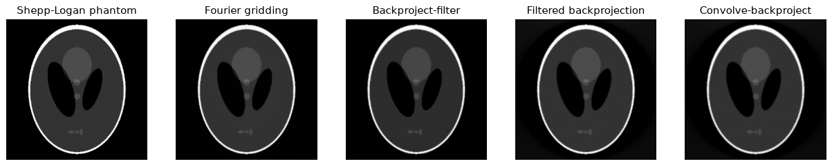
|
+
|
|
3
|
+
Copyright (c) 2023 GivralNguyen
|
|
4
|
+
|
|
5
|
+
Permission is hereby granted, free of charge, to any person obtaining a copy
|
|
6
|
+
of this software and associated documentation files (the "Software"), to deal
|
|
7
|
+
in the Software without restriction, including without limitation the rights
|
|
8
|
+
to use, copy, modify, merge, publish, distribute, sublicense, and/or sell
|
|
9
|
+
copies of the Software, and to permit persons to whom the Software is
|
|
10
|
+
furnished to do so, subject to the following conditions:
|
|
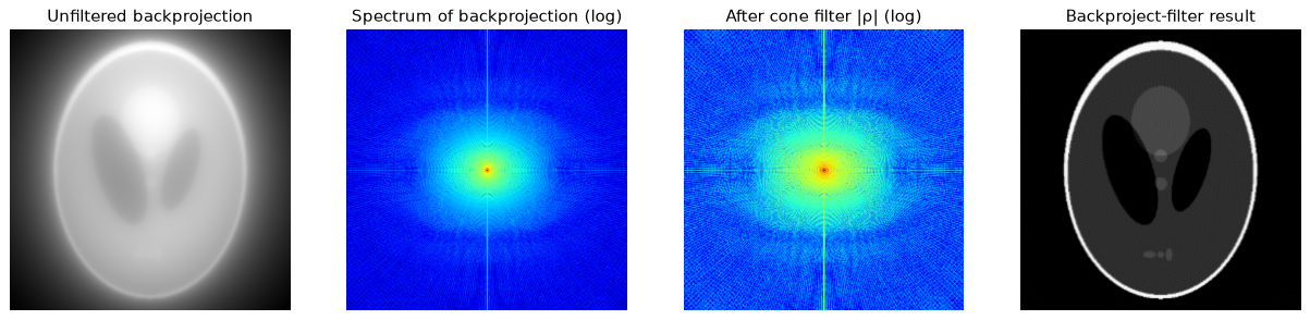
11
|
+
|
|
12
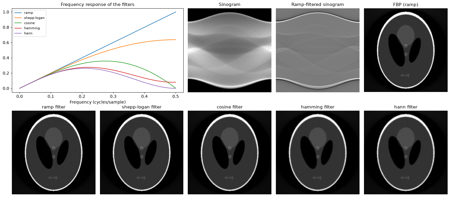
|
+
The above copyright notice and this permission notice shall be included in all
|
|
13
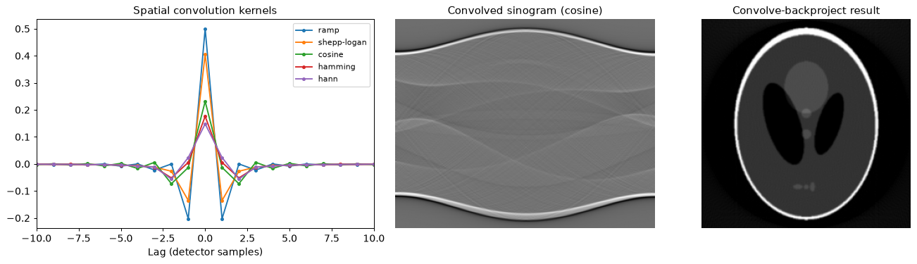
|
+
copies or substantial portions of the Software.
|
|
14
|
+
|
|
15
|
+
THE SOFTWARE IS PROVIDED "AS IS", WITHOUT WARRANTY OF ANY KIND, EXPRESS OR
|
|
16
|
+
IMPLIED, INCLUDING BUT NOT LIMITED TO THE WARRANTIES OF MERCHANTABILITY,
|
|
17
|
+
FITNESS FOR A PARTICULAR PURPOSE AND NONINFRINGEMENT. IN NO EVENT SHALL THE
|
|
18
|
+
AUTHORS OR COPYRIGHT HOLDERS BE LIABLE FOR ANY CLAIM, DAMAGES OR OTHER
|
|
19
|
+
LIABILITY, WHETHER IN AN ACTION OF CONTRACT, TORT OR OTHERWISE, ARISING FROM,
|
|
20
|
+
OUT OF OR IN CONNECTION WITH THE SOFTWARE OR THE USE OR OTHER DEALINGS IN THE
|
|
21
|
+
SOFTWARE.
|
tomorecon-0.1.0/PKG-INFO
ADDED
|
@@ -0,0 +1,158 @@
|
|
|
1
|
+
Metadata-Version: 2.5
|
|
2
|
+
Name: tomorecon
|
|
3
|
+
Version: 0.1.0
|
|
4
|
+
Summary: Analytical tomographic image reconstruction: Radon transform, Fourier gridding, filtered backprojection, backproject-filter and convolve-backproject.
|
|
5
|
+
Project-URL: Homepage, https://github.com/GivralNguyen/Python-Medical-Analytical-Tomographic-Image-Reconstruction
|
|
6
|
+
Author: GivralNguyen
|
|
7
|
+
License-Expression: MIT
|
|
8
|
+
License-File: LICENSE
|
|
9
|
+
Keywords: computed tomography,filtered backprojection,image reconstruction,radon transform,tomography
|
|
10
|
+
Classifier: Intended Audience :: Education
|
|
11
|
+
Classifier: Intended Audience :: Science/Research
|
|
12
|
+
Classifier: Operating System :: OS Independent
|
|
13
|
+
Classifier: Programming Language :: Python :: 3
|
|
14
|
+
Classifier: Topic :: Scientific/Engineering :: Image Processing
|
|
15
|
+
Classifier: Topic :: Scientific/Engineering :: Medical Science Apps.
|
|
16
|
+
Requires-Python: >=3.9
|
|
17
|
+
Requires-Dist: imageio>=2.16
|
|
18
|
+
Requires-Dist: numpy>=1.21
|
|
19
|
+
Requires-Dist: scikit-image>=0.19
|
|
20
|
+
Requires-Dist: scipy>=1.8
|
|
21
|
+
Provides-Extra: notebook
|
|
22
|
+
Requires-Dist: jupyter; extra == 'notebook'
|
|
23
|
+
Requires-Dist: matplotlib; extra == 'notebook'
|
|
24
|
+
Provides-Extra: test
|
|
25
|
+
Requires-Dist: pytest; extra == 'test'
|
|
26
|
+
Description-Content-Type: text/markdown
|
|
27
|
+
|
|
28
|
+
# Analytical Tomographic Image Reconstruction
|
|
29
|
+
|
|
30
|
+
Welcome to the Analytical Tomographic Image Reconstruction repository! This collection of Python code provides implementations for various analytical tomographic image reconstruction algorithms. These algorithms play a crucial role in transforming projection data into detailed images, making them valuable tools in medical imaging, materials science, and more. Included are **Fourier Gridding**, **Backproject Filter**, **Filtered Backprojection** and **Convolve Backproject**.
|
|
31
|
+
|
|
32
|
+
|
|
33
|
+
|
|
34
|
+
## Installation
|
|
35
|
+
|
|
36
|
+
```bash
|
|
37
|
+
pip install git+https://github.com/GivralNguyen/Python-Medical-Analytical-Tomographic-Image-Reconstruction.git
|
|
38
|
+
```
|
|
39
|
+
|
|
40
|
+
Or from a local clone (editable, with the extras for the notebook and tests):
|
|
41
|
+
|
|
42
|
+
```bash
|
|
43
|
+
git clone https://github.com/GivralNguyen/Python-Medical-Analytical-Tomographic-Image-Reconstruction.git
|
|
44
|
+
cd Python-Medical-Analytical-Tomographic-Image-Reconstruction
|
|
45
|
+
pip install -e ".[notebook,test]"
|
|
46
|
+
```
|
|
47
|
+
|
|
48
|
+
Requires Python ≥ 3.9; dependencies (numpy, scipy, scikit-image, imageio) are installed automatically.
|
|
49
|
+
|
|
50
|
+
## Quick Start
|
|
51
|
+
|
|
52
|
+
```python
|
|
53
|
+
import numpy as np
|
|
54
|
+
import tomorecon as tr
|
|
55
|
+
|
|
56
|
+
phantom = tr.shepp_logan() # 256 x 256, bundled with the package
|
|
57
|
+
theta = np.arange(180) # projection angles in degrees
|
|
58
|
+
sinogram = tr.radon(phantom, theta) # shape (256, 180): one projection per column
|
|
59
|
+
|
|
60
|
+
image = tr.fbp(sinogram, theta) # filtered backprojection
|
|
61
|
+
image = tr.fbp(sinogram, theta, filter="hann") # 'ramp', 'shepp-logan', 'cosine', 'hamming', 'hann'
|
|
62
|
+
image = tr.cbp(sinogram, theta) # convolve-backproject (spatial-domain filtering)
|
|
63
|
+
image = tr.bpf(sinogram, theta) # backproject-filter (2-D cone filter)
|
|
64
|
+
image = tr.fourier_gridding(sinogram, theta) # direct Fourier reconstruction
|
|
65
|
+
image = tr.backproject(sinogram, theta) # unfiltered backprojection (blurred)
|
|
66
|
+
```
|
|
67
|
+
|
|
68
|
+
Every step is also available on its own, e.g. `tr.filter_sinogram`, `tr.convolve_sinogram`, `tr.spatial_kernel`, `tr.cone_filter`, `tr.projection_spectra`, `tr.polar_to_cartesian` and `tr.inverse_fft2`. See the [tutorial](https://github.com/GivralNguyen/Python-Medical-Analytical-Tomographic-Image-Reconstruction/blob/main/tutorial.ipynb) for how they fit together.
|
|
69
|
+
|
|
70
|
+
### API
|
|
71
|
+
|
|
72
|
+
| Function | Description |
|
|
73
|
+
|---|---|
|
|
74
|
+
| `shepp_logan(size=256)`, `disk(...)`, `load_image(path, size=256)` | Test objects |
|
|
75
|
+
| `radon(image, theta=None, circle=True)` | Sinogram, shape `(n_detectors, n_angles)` |
|
|
76
|
+
| `backproject(sinogram, theta=None, output_size=None, interval=1)` | Unfiltered backprojection |
|
|
77
|
+
| `fbp(sinogram, theta=None, filter="ramp", output_size=None)` | Filtered backprojection |
|
|
78
|
+
| `cbp(sinogram, theta=None, filter="ramp", output_size=None)` | Convolve-backproject |
|
|
79
|
+
| `bpf(sinogram, theta=None, filter="ramp", output_size=None, grid_factor=2)` | Backproject-filter |
|
|
80
|
+
| `fourier_gridding(sinogram, theta=None, output_size=None, oversample=4)` | Direct Fourier reconstruction |
|
|
81
|
+
|
|
82
|
+
Angles are in degrees; if `theta` is omitted, the projections are assumed equally spaced over [0°, 180°).
|
|
83
|
+
|
|
84
|
+
## Sample Results
|
|
85
|
+
|
|
86
|
+
All images below are produced from the 256×256 Shepp-Logan phantom with 180 projections (0°–179°), using the code in this repository. See [tutorial.ipynb](https://github.com/GivralNguyen/Python-Medical-Analytical-Tomographic-Image-Reconstruction/blob/main/tutorial.ipynb) for the full walkthrough.
|
|
87
|
+
|
|
88
|
+
### Radon Transform
|
|
89
|
+
|
|
90
|
+
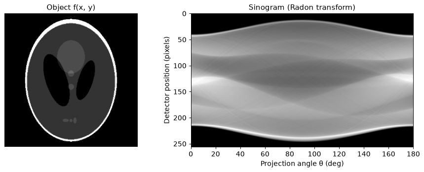
Each column of the sinogram is one projection: the line integrals of the object along parallel rays at angle θ.
|
|
91
|
+
|
|
92
|
+
|
|
93
|
+
|
|
94
|
+
### Fourier Gridding
|
|
95
|
+
|
|
96
|
+
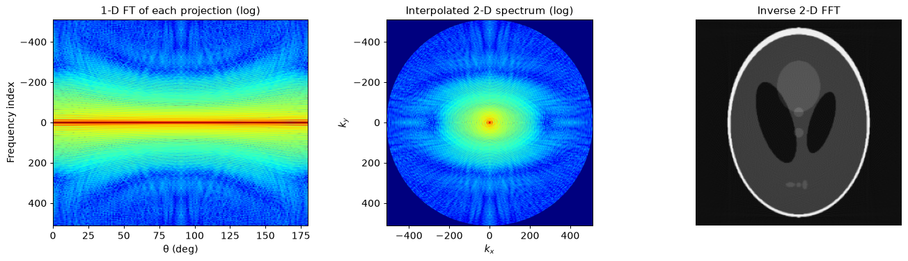
By the Fourier slice theorem, the 1-D Fourier transform of a projection at angle θ is a radial line through the 2-D Fourier transform of the object. The slices are interpolated from the polar grid onto a Cartesian grid, and an inverse 2-D FFT gives the image. The projections are zero-padded 4× first (oversampling), which keeps the interpolation error small.
|
|
97
|
+
|
|
98
|
+
|
|
99
|
+
|
|
100
|
+
### Backprojection
|
|
101
|
+
|
|
102
|
+
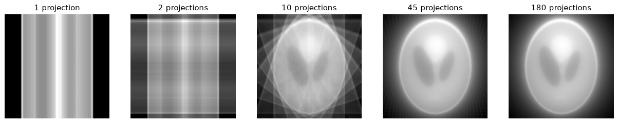
Smearing every projection back across the image plane. With few angles the streaks are obvious; with all 180 angles the result is the object blurred by 1/r.
|
|
103
|
+
|
|
104
|
+
|
|
105
|
+
|
|
106
|
+
### Backproject Filter
|
|
107
|
+
|
|
108
|
+
The 1/r blur of the backprojection is removed afterwards in 2-D: multiply its spectrum by the cone filter |ρ| and transform back. The backprojection is computed on a 2× larger grid, since the blur extends far outside the object.
|
|
109
|
+
|
|
110
|
+
|
|
111
|
+
|
|
112
|
+
### Filtered Backprojection
|
|
113
|
+
|
|
114
|
+
Each projection is filtered with a 1-D ramp filter |ω| (optionally apodized) before backprojection. Smoother windows trade resolution for less noise.
|
|
115
|
+
|
|
116
|
+
|
|
117
|
+
|
|
118
|
+
### Convolve Backproject
|
|
119
|
+
|
|
120
|
+
The same filtering as FBP, but done in the spatial domain by convolving each projection with the inverse Fourier transform of the filter. The result is identical to FBP up to floating-point error.
|
|
121
|
+
|
|
122
|
+
|
|
123
|
+
|
|
124
|
+
## Code Structure
|
|
125
|
+
|
|
126
|
+
The package lives in `src/tomorecon/`:
|
|
127
|
+
|
|
128
|
+
| Module | Contents |
|
|
129
|
+
|---|---|
|
|
130
|
+
| `phantoms.py` | `shepp_logan`, `disk`, `load_image` |
|
|
131
|
+
| `projection.py` | `radon`: the forward model |
|
|
132
|
+
| `backprojection.py` | `backproject`, `fbp`, `cbp`, `bpf` |
|
|
133
|
+
| `filters.py` | Ramp-type filters (`fourier_filter`), their spatial kernels (`spatial_kernel`), `filter_sinogram`, `convolve_sinogram` and the 2-D `cone_filter` |
|
|
134
|
+
| `gridding.py` | `fourier_gridding` and its steps: `projection_spectra`, `polar_to_cartesian`, `inverse_fft2`, `polar_grid`, `cartesian_grid` |
|
|
135
|
+
|
|
136
|
+
Outside the package:
|
|
137
|
+
|
|
138
|
+
- **tutorial.ipynb**: Jupyter notebook demonstrating the usage of all reconstruction methods with examples and visualizations.
|
|
139
|
+
- **tests/**: checks that every method reconstructs the phantom accurately (run `pytest`).
|
|
140
|
+
- **data/**: extra sample images for `load_image`.
|
|
141
|
+
|
|
142
|
+
## Tutorial
|
|
143
|
+
|
|
144
|
+
After installing with the `notebook` extra, explore the provided [tutorial.ipynb](https://github.com/GivralNguyen/Python-Medical-Analytical-Tomographic-Image-Reconstruction/blob/main/tutorial.ipynb) notebook for comprehensive examples and visualizations of each reconstruction method. You can experiment with different data sources and filters to see how these algorithms perform under various conditions.
|
|
145
|
+
|
|
146
|
+
## Contributing
|
|
147
|
+
|
|
148
|
+
We welcome contributions to enhance and expand this repository. If you have improvements, additional algorithms, or new features to suggest, please feel free to open an issue or submit a pull request.
|
|
149
|
+
|
|
150
|
+
## Acknowledgments
|
|
151
|
+
|
|
152
|
+
Special thanks to me for writing this and Prof. Lasser for the wonderful Seminar course
|
|
153
|
+
|
|
154
|
+
## License
|
|
155
|
+
|
|
156
|
+
This code is released under the [MIT License](https://github.com/GivralNguyen/Python-Medical-Analytical-Tomographic-Image-Reconstruction/blob/main/LICENSE). Feel free to use, modify, and distribute the code in accordance with the terms of the license.
|
|
157
|
+
|
|
158
|
+
Happy reconstructing! 🌐🖼️
|
|
@@ -0,0 +1,131 @@
|
|
|
1
|
+
# Analytical Tomographic Image Reconstruction
|
|
2
|
+
|
|
3
|
+
Welcome to the Analytical Tomographic Image Reconstruction repository! This collection of Python code provides implementations for various analytical tomographic image reconstruction algorithms. These algorithms play a crucial role in transforming projection data into detailed images, making them valuable tools in medical imaging, materials science, and more. Included are **Fourier Gridding**, **Backproject Filter**, **Filtered Backprojection** and **Convolve Backproject**.
|
|
4
|
+
|
|
5
|
+

|
|
6
|
+
|
|
7
|
+
## Installation
|
|
8
|
+
|
|
9
|
+
```bash
|
|
10
|
+
pip install git+https://github.com/GivralNguyen/Python-Medical-Analytical-Tomographic-Image-Reconstruction.git
|
|
11
|
+
```
|
|
12
|
+
|
|
13
|
+
Or from a local clone (editable, with the extras for the notebook and tests):
|
|
14
|
+
|
|
15
|
+
```bash
|
|
16
|
+
git clone https://github.com/GivralNguyen/Python-Medical-Analytical-Tomographic-Image-Reconstruction.git
|
|
17
|
+
cd Python-Medical-Analytical-Tomographic-Image-Reconstruction
|
|
18
|
+
pip install -e ".[notebook,test]"
|
|
19
|
+
```
|
|
20
|
+
|
|
21
|
+
Requires Python ≥ 3.9; dependencies (numpy, scipy, scikit-image, imageio) are installed automatically.
|
|
22
|
+
|
|
23
|
+
## Quick Start
|
|
24
|
+
|
|
25
|
+
```python
|
|
26
|
+
import numpy as np
|
|
27
|
+
import tomorecon as tr
|
|
28
|
+
|
|
29
|
+
phantom = tr.shepp_logan() # 256 x 256, bundled with the package
|
|
30
|
+
theta = np.arange(180) # projection angles in degrees
|
|
31
|
+
sinogram = tr.radon(phantom, theta) # shape (256, 180): one projection per column
|
|
32
|
+
|
|
33
|
+
image = tr.fbp(sinogram, theta) # filtered backprojection
|
|
34
|
+
image = tr.fbp(sinogram, theta, filter="hann") # 'ramp', 'shepp-logan', 'cosine', 'hamming', 'hann'
|
|
35
|
+
image = tr.cbp(sinogram, theta) # convolve-backproject (spatial-domain filtering)
|
|
36
|
+
image = tr.bpf(sinogram, theta) # backproject-filter (2-D cone filter)
|
|
37
|
+
image = tr.fourier_gridding(sinogram, theta) # direct Fourier reconstruction
|
|
38
|
+
image = tr.backproject(sinogram, theta) # unfiltered backprojection (blurred)
|
|
39
|
+
```
|
|
40
|
+
|
|
41
|
+
Every step is also available on its own, e.g. `tr.filter_sinogram`, `tr.convolve_sinogram`, `tr.spatial_kernel`, `tr.cone_filter`, `tr.projection_spectra`, `tr.polar_to_cartesian` and `tr.inverse_fft2`. See the [tutorial](https://github.com/GivralNguyen/Python-Medical-Analytical-Tomographic-Image-Reconstruction/blob/main/tutorial.ipynb) for how they fit together.
|
|
42
|
+
|
|
43
|
+
### API
|
|
44
|
+
|
|
45
|
+
| Function | Description |
|
|
46
|
+
|---|---|
|
|
47
|
+
| `shepp_logan(size=256)`, `disk(...)`, `load_image(path, size=256)` | Test objects |
|
|
48
|
+
| `radon(image, theta=None, circle=True)` | Sinogram, shape `(n_detectors, n_angles)` |
|
|
49
|
+
| `backproject(sinogram, theta=None, output_size=None, interval=1)` | Unfiltered backprojection |
|
|
50
|
+
| `fbp(sinogram, theta=None, filter="ramp", output_size=None)` | Filtered backprojection |
|
|
51
|
+
| `cbp(sinogram, theta=None, filter="ramp", output_size=None)` | Convolve-backproject |
|
|
52
|
+
| `bpf(sinogram, theta=None, filter="ramp", output_size=None, grid_factor=2)` | Backproject-filter |
|
|
53
|
+
| `fourier_gridding(sinogram, theta=None, output_size=None, oversample=4)` | Direct Fourier reconstruction |
|
|
54
|
+
|
|
55
|
+
Angles are in degrees; if `theta` is omitted, the projections are assumed equally spaced over [0°, 180°).
|
|
56
|
+
|
|
57
|
+
## Sample Results
|
|
58
|
+
|
|
59
|
+
All images below are produced from the 256×256 Shepp-Logan phantom with 180 projections (0°–179°), using the code in this repository. See [tutorial.ipynb](https://github.com/GivralNguyen/Python-Medical-Analytical-Tomographic-Image-Reconstruction/blob/main/tutorial.ipynb) for the full walkthrough.
|
|
60
|
+
|
|
61
|
+
### Radon Transform
|
|
62
|
+
|
|
63
|
+
Each column of the sinogram is one projection: the line integrals of the object along parallel rays at angle θ.
|
|
64
|
+
|
|
65
|
+

|
|
66
|
+
|
|
67
|
+
### Fourier Gridding
|
|
68
|
+
|
|
69
|
+
By the Fourier slice theorem, the 1-D Fourier transform of a projection at angle θ is a radial line through the 2-D Fourier transform of the object. The slices are interpolated from the polar grid onto a Cartesian grid, and an inverse 2-D FFT gives the image. The projections are zero-padded 4× first (oversampling), which keeps the interpolation error small.
|
|
70
|
+
|
|
71
|
+

|
|
72
|
+
|
|
73
|
+
### Backprojection
|
|
74
|
+
|
|
75
|
+
Smearing every projection back across the image plane. With few angles the streaks are obvious; with all 180 angles the result is the object blurred by 1/r.
|
|
76
|
+
|
|
77
|
+

|
|
78
|
+
|
|
79
|
+
### Backproject Filter
|
|
80
|
+
|
|
81
|
+
The 1/r blur of the backprojection is removed afterwards in 2-D: multiply its spectrum by the cone filter |ρ| and transform back. The backprojection is computed on a 2× larger grid, since the blur extends far outside the object.
|
|
82
|
+
|
|
83
|
+

|
|
84
|
+
|
|
85
|
+
### Filtered Backprojection
|
|
86
|
+
|
|
87
|
+
Each projection is filtered with a 1-D ramp filter |ω| (optionally apodized) before backprojection. Smoother windows trade resolution for less noise.
|
|
88
|
+
|
|
89
|
+

|
|
90
|
+
|
|
91
|
+
### Convolve Backproject
|
|
92
|
+
|
|
93
|
+
The same filtering as FBP, but done in the spatial domain by convolving each projection with the inverse Fourier transform of the filter. The result is identical to FBP up to floating-point error.
|
|
94
|
+
|
|
95
|
+

|
|
96
|
+
|
|
97
|
+
## Code Structure
|
|
98
|
+
|
|
99
|
+
The package lives in `src/tomorecon/`:
|
|
100
|
+
|
|
101
|
+
| Module | Contents |
|
|
102
|
+
|---|---|
|
|
103
|
+
| `phantoms.py` | `shepp_logan`, `disk`, `load_image` |
|
|
104
|
+
| `projection.py` | `radon`: the forward model |
|
|
105
|
+
| `backprojection.py` | `backproject`, `fbp`, `cbp`, `bpf` |
|
|
106
|
+
| `filters.py` | Ramp-type filters (`fourier_filter`), their spatial kernels (`spatial_kernel`), `filter_sinogram`, `convolve_sinogram` and the 2-D `cone_filter` |
|
|
107
|
+
| `gridding.py` | `fourier_gridding` and its steps: `projection_spectra`, `polar_to_cartesian`, `inverse_fft2`, `polar_grid`, `cartesian_grid` |
|
|
108
|
+
|
|
109
|
+
Outside the package:
|
|
110
|
+
|
|
111
|
+
- **tutorial.ipynb**: Jupyter notebook demonstrating the usage of all reconstruction methods with examples and visualizations.
|
|
112
|
+
- **tests/**: checks that every method reconstructs the phantom accurately (run `pytest`).
|
|
113
|
+
- **data/**: extra sample images for `load_image`.
|
|
114
|
+
|
|
115
|
+
## Tutorial
|
|
116
|
+
|
|
117
|
+
After installing with the `notebook` extra, explore the provided [tutorial.ipynb](https://github.com/GivralNguyen/Python-Medical-Analytical-Tomographic-Image-Reconstruction/blob/main/tutorial.ipynb) notebook for comprehensive examples and visualizations of each reconstruction method. You can experiment with different data sources and filters to see how these algorithms perform under various conditions.
|
|
118
|
+
|
|
119
|
+
## Contributing
|
|
120
|
+
|
|
121
|
+
We welcome contributions to enhance and expand this repository. If you have improvements, additional algorithms, or new features to suggest, please feel free to open an issue or submit a pull request.
|
|
122
|
+
|
|
123
|
+
## Acknowledgments
|
|
124
|
+
|
|
125
|
+
Special thanks to me for writing this and Prof. Lasser for the wonderful Seminar course
|
|
126
|
+
|
|
127
|
+
## License
|
|
128
|
+
|
|
129
|
+
This code is released under the [MIT License](https://github.com/GivralNguyen/Python-Medical-Analytical-Tomographic-Image-Reconstruction/blob/main/LICENSE). Feel free to use, modify, and distribute the code in accordance with the terms of the license.
|
|
130
|
+
|
|
131
|
+
Happy reconstructing! 🌐🖼️
|
|
@@ -0,0 +1,41 @@
|
|
|
1
|
+
[build-system]
|
|
2
|
+
requires = ["hatchling>=1.26"]
|
|
3
|
+
build-backend = "hatchling.build"
|
|
4
|
+
|
|
5
|
+
[project]
|
|
6
|
+
name = "tomorecon"
|
|
7
|
+
version = "0.1.0"
|
|
8
|
+
description = "Analytical tomographic image reconstruction: Radon transform, Fourier gridding, filtered backprojection, backproject-filter and convolve-backproject."
|
|
9
|
+
readme = "README.md"
|
|
10
|
+
requires-python = ">=3.9"
|
|
11
|
+
license = "MIT"
|
|
12
|
+
license-files = ["LICENSE"]
|
|
13
|
+
authors = [{ name = "GivralNguyen" }]
|
|
14
|
+
keywords = ["tomography", "computed tomography", "image reconstruction", "radon transform", "filtered backprojection"]
|
|
15
|
+
classifiers = [
|
|
16
|
+
"Programming Language :: Python :: 3",
|
|
17
|
+
"Operating System :: OS Independent",
|
|
18
|
+
"Intended Audience :: Science/Research",
|
|
19
|
+
"Intended Audience :: Education",
|
|
20
|
+
"Topic :: Scientific/Engineering :: Image Processing",
|
|
21
|
+
"Topic :: Scientific/Engineering :: Medical Science Apps.",
|
|
22
|
+
]
|
|
23
|
+
dependencies = [
|
|
24
|
+
"numpy>=1.21",
|
|
25
|
+
"scipy>=1.8",
|
|
26
|
+
"scikit-image>=0.19",
|
|
27
|
+
"imageio>=2.16",
|
|
28
|
+
]
|
|
29
|
+
|
|
30
|
+
[project.optional-dependencies]
|
|
31
|
+
notebook = ["matplotlib", "jupyter"]
|
|
32
|
+
test = ["pytest"]
|
|
33
|
+
|
|
34
|
+
[project.urls]
|
|
35
|
+
Homepage = "https://github.com/GivralNguyen/Python-Medical-Analytical-Tomographic-Image-Reconstruction"
|
|
36
|
+
|
|
37
|
+
[tool.hatch.build.targets.wheel]
|
|
38
|
+
packages = ["src/tomorecon"]
|
|
39
|
+
|
|
40
|
+
[tool.hatch.build.targets.sdist]
|
|
41
|
+
include = ["src/tomorecon", "tests", "README.md", "LICENSE", "pyproject.toml"]
|
|
@@ -0,0 +1,52 @@
|
|
|
1
|
+
"""
|
|
2
|
+
tomorecon: analytical tomographic image reconstruction.
|
|
3
|
+
|
|
4
|
+
Radon transform, Fourier gridding, (filtered) backprojection, backproject-filter
|
|
5
|
+
and convolve-backproject for 2-D parallel-beam tomography.
|
|
6
|
+
|
|
7
|
+
Example
|
|
8
|
+
-------
|
|
9
|
+
>>> import tomorecon as tr
|
|
10
|
+
>>> phantom = tr.shepp_logan()
|
|
11
|
+
>>> sinogram = tr.radon(phantom) # 180 angles, 0..179 degrees
|
|
12
|
+
>>> image = tr.fbp(sinogram) # ramp-filtered backprojection
|
|
13
|
+
"""
|
|
14
|
+
|
|
15
|
+
from .backprojection import backproject, bpf, cbp, fbp
|
|
16
|
+
from .filters import (
|
|
17
|
+
FILTERS,
|
|
18
|
+
cone_filter,
|
|
19
|
+
convolve_sinogram,
|
|
20
|
+
filter_sinogram,
|
|
21
|
+
fourier_filter,
|
|
22
|
+
padded_size,
|
|
23
|
+
spatial_kernel,
|
|
24
|
+
)
|
|
25
|
+
from .gridding import (
|
|
26
|
+
cartesian_grid,
|
|
27
|
+
fourier_gridding,
|
|
28
|
+
frequency_axis,
|
|
29
|
+
inverse_fft2,
|
|
30
|
+
polar_grid,
|
|
31
|
+
polar_to_cartesian,
|
|
32
|
+
projection_spectra,
|
|
33
|
+
)
|
|
34
|
+
from .phantoms import disk, load_image, shepp_logan
|
|
35
|
+
from .projection import radon
|
|
36
|
+
|
|
37
|
+
__version__ = "0.1.0"
|
|
38
|
+
|
|
39
|
+
__all__ = [
|
|
40
|
+
# data
|
|
41
|
+
"shepp_logan", "disk", "load_image",
|
|
42
|
+
# forward model
|
|
43
|
+
"radon",
|
|
44
|
+
# reconstruction
|
|
45
|
+
"backproject", "fbp", "cbp", "bpf", "fourier_gridding",
|
|
46
|
+
# filters
|
|
47
|
+
"FILTERS", "fourier_filter", "spatial_kernel", "filter_sinogram", "convolve_sinogram",
|
|
48
|
+
"cone_filter", "padded_size",
|
|
49
|
+
# Fourier gridding steps
|
|
50
|
+
"projection_spectra", "polar_to_cartesian", "inverse_fft2", "polar_grid", "cartesian_grid",
|
|
51
|
+
"frequency_axis",
|
|
52
|
+
]
|
|
@@ -0,0 +1,31 @@
|
|
|
1
|
+
from __future__ import annotations
|
|
2
|
+
|
|
3
|
+
import numpy as np
|
|
4
|
+
from skimage.util import img_as_float
|
|
5
|
+
|
|
6
|
+
|
|
7
|
+
def as_float_image(image) -> np.ndarray:
|
|
8
|
+
"""Image as float; integer/bool images are rescaled to [0, 1] like skimage's `img_as_float`."""
|
|
9
|
+
image = np.asarray(image)
|
|
10
|
+
if image.dtype == np.float16:
|
|
11
|
+
return image.astype(np.float32)
|
|
12
|
+
return img_as_float(image)
|
|
13
|
+
|
|
14
|
+
|
|
15
|
+
def as_float_data(data) -> np.ndarray:
|
|
16
|
+
"""Measured data (e.g. a sinogram) as float, keeping its values."""
|
|
17
|
+
data = np.asarray(data)
|
|
18
|
+
if data.dtype.char not in "df":
|
|
19
|
+
data = data.astype(np.float32 if data.dtype == np.float16 else float)
|
|
20
|
+
return data
|
|
21
|
+
|
|
22
|
+
|
|
23
|
+
def default_theta(n_angles: int) -> np.ndarray:
|
|
24
|
+
"""`n_angles` equally spaced angles in [0, 180) degrees."""
|
|
25
|
+
return np.linspace(0, 180, n_angles, endpoint=False)
|
|
26
|
+
|
|
27
|
+
|
|
28
|
+
def center_crop(image: np.ndarray, size: int) -> np.ndarray:
|
|
29
|
+
"""Centred size x size crop of a square image (centre pixel at index shape // 2)."""
|
|
30
|
+
start = image.shape[0] // 2 - size // 2
|
|
31
|
+
return image[start:start + size, start:start + size]
|
|
@@ -0,0 +1,95 @@
|
|
|
1
|
+
"""Backprojection-based reconstruction: BP, FBP, CBP and BPF."""
|
|
2
|
+
from __future__ import annotations
|
|
3
|
+
|
|
4
|
+
import numpy as np
|
|
5
|
+
|
|
6
|
+
from ._utils import as_float_data, default_theta
|
|
7
|
+
from .filters import cone_filter, convolve_sinogram, filter_sinogram
|
|
8
|
+
|
|
9
|
+
__all__ = ["backproject", "fbp", "cbp", "bpf"]
|
|
10
|
+
|
|
11
|
+
|
|
12
|
+
def _angles(sinogram, theta):
|
|
13
|
+
if theta is None:
|
|
14
|
+
return default_theta(sinogram.shape[1])
|
|
15
|
+
theta = np.asarray(theta, dtype=float)
|
|
16
|
+
if theta.shape != (sinogram.shape[1],):
|
|
17
|
+
raise ValueError(f"theta has {theta.size} angles but the sinogram has {sinogram.shape[1]} columns")
|
|
18
|
+
return theta
|
|
19
|
+
|
|
20
|
+
|
|
21
|
+
def backproject(sinogram: np.ndarray, theta: np.ndarray | None = None,
|
|
22
|
+
output_size: int | None = None, interval: int = 1) -> np.ndarray:
|
|
23
|
+
"""
|
|
24
|
+
Unfiltered backprojection: smear every projection back across the image plane.
|
|
25
|
+
|
|
26
|
+
Parameters
|
|
27
|
+
----------
|
|
28
|
+
sinogram : ndarray of shape (n_detectors, n_angles)
|
|
29
|
+
As returned by `radon`; rotation centre at row n_detectors // 2.
|
|
30
|
+
theta : 1-D array, optional
|
|
31
|
+
Projection angles in degrees. Default: n_angles equally spaced angles in [0, 180).
|
|
32
|
+
output_size : int, optional
|
|
33
|
+
Side of the reconstructed image. Default: n_detectors.
|
|
34
|
+
interval : int
|
|
35
|
+
Use only every `interval`-th projection (to show the effect of fewer angles).
|
|
36
|
+
|
|
37
|
+
Returns
|
|
38
|
+
-------
|
|
39
|
+
ndarray of shape (output_size, output_size)
|
|
40
|
+
Scaled by pi / (2 * angles used), so that backprojecting a ramp-filtered
|
|
41
|
+
sinogram reconstructs the object at its original intensity.
|
|
42
|
+
"""
|
|
43
|
+
sinogram = as_float_data(sinogram)
|
|
44
|
+
theta = _angles(sinogram, theta)
|
|
45
|
+
n = sinogram.shape[0]
|
|
46
|
+
output_size = output_size or n
|
|
47
|
+
|
|
48
|
+
rows, cols = np.mgrid[:output_size, :output_size] - output_size // 2
|
|
49
|
+
detector = np.arange(n) - n // 2
|
|
50
|
+
image = np.zeros((output_size, output_size))
|
|
51
|
+
used = range(0, len(theta), interval)
|
|
52
|
+
for i in used:
|
|
53
|
+
angle = np.deg2rad(theta[i])
|
|
54
|
+
t = cols * np.cos(angle) - rows * np.sin(angle)
|
|
55
|
+
image += np.interp(t, detector, sinogram[:, i], left=0, right=0)
|
|
56
|
+
return image * np.pi / (2 * len(used))
|
|
57
|
+
|
|
58
|
+
|
|
59
|
+
def fbp(sinogram: np.ndarray, theta: np.ndarray | None = None, filter: str | None = "ramp",
|
|
60
|
+
output_size: int | None = None) -> np.ndarray:
|
|
61
|
+
"""
|
|
62
|
+
Filtered backprojection: filter every projection in the frequency domain, then backproject.
|
|
63
|
+
|
|
64
|
+
`filter` is one of `FILTERS` ('ramp', 'shepp-logan', 'cosine', 'hamming', 'hann');
|
|
65
|
+
smoother windows trade resolution for less noise. See `backproject` for the other arguments.
|
|
66
|
+
"""
|
|
67
|
+
return backproject(filter_sinogram(sinogram, filter), theta, output_size)
|
|
68
|
+
|
|
69
|
+
|
|
70
|
+
def cbp(sinogram: np.ndarray, theta: np.ndarray | None = None, filter: str | None = "ramp",
|
|
71
|
+
output_size: int | None = None) -> np.ndarray:
|
|
72
|
+
"""
|
|
73
|
+
Convolve-backproject: like `fbp`, but the filter is applied as a spatial convolution
|
|
74
|
+
of each projection. The result is identical to `fbp` up to floating-point error.
|
|
75
|
+
"""
|
|
76
|
+
return backproject(convolve_sinogram(sinogram, filter), theta, output_size)
|
|
77
|
+
|
|
78
|
+
|
|
79
|
+
def bpf(sinogram: np.ndarray, theta: np.ndarray | None = None, filter: str | None = "ramp",
|
|
80
|
+
output_size: int | None = None, grid_factor: int = 2) -> np.ndarray:
|
|
81
|
+
"""
|
|
82
|
+
Backproject-filter: backproject first, then remove the 1/r blur with the 2-D cone filter.
|
|
83
|
+
|
|
84
|
+
Parameters
|
|
85
|
+
----------
|
|
86
|
+
grid_factor : int
|
|
87
|
+
Backproject onto a grid `grid_factor` times larger than `output_size` before
|
|
88
|
+
filtering, because the 1/r blur extends far outside the object (1 gives visible
|
|
89
|
+
errors; 2 is enough in practice).
|
|
90
|
+
|
|
91
|
+
See `backproject` and `fbp` for the other arguments.
|
|
92
|
+
"""
|
|
93
|
+
output_size = output_size or np.asarray(sinogram).shape[0]
|
|
94
|
+
blurred = backproject(sinogram, theta, grid_factor * output_size)
|
|
95
|
+
return cone_filter(blurred, filter, output_size)[1]
|
|
Binary file
|
|
@@ -0,0 +1,163 @@
|
|
|
1
|
+
"""Reconstruction filters: 1-D ramp-type filters, their spatial kernels, and the 2-D cone filter."""
|
|
2
|
+
from __future__ import annotations
|
|
3
|
+
|
|
4
|
+
import numpy as np
|
|
5
|
+
from scipy.fft import fft, fft2, fftfreq, fftshift, ifft, ifft2
|
|
6
|
+
|
|
7
|
+
from ._utils import as_float_data, center_crop
|
|
8
|
+
|
|
9
|
+
__all__ = [
|
|
10
|
+
"FILTERS",
|
|
11
|
+
"padded_size",
|
|
12
|
+
"fourier_filter",
|
|
13
|
+
"spatial_kernel",
|
|
14
|
+
"filter_sinogram",
|
|
15
|
+
"convolve_sinogram",
|
|
16
|
+
"cone_filter",
|
|
17
|
+
]
|
|
18
|
+
|
|
19
|
+
FILTERS = ("ramp", "shepp-logan", "cosine", "hamming", "hann")
|
|
20
|
+
|
|
21
|
+
|
|
22
|
+
def _check(name):
|
|
23
|
+
if name is not None and name not in FILTERS:
|
|
24
|
+
raise ValueError(f"Unknown filter {name!r}; choose one of {FILTERS} or None")
|
|
25
|
+
|
|
26
|
+
|
|
27
|
+
def padded_size(n: int) -> int:
|
|
28
|
+
"""Smallest power of two >= 2n (and >= 64): FFT filtering at this length is a linear convolution."""
|
|
29
|
+
return max(64, int(2 ** np.ceil(np.log2(2 * n))))
|
|
30
|
+
|
|
31
|
+
|
|
32
|
+
def fourier_filter(size: int, name: str | None = "ramp") -> np.ndarray:
|
|
33
|
+
"""
|
|
34
|
+
Frequency response of a reconstruction filter, in FFT order (DC first).
|
|
35
|
+
|
|
36
|
+
The ramp is built as the DFT of the band-limited spatial ramp kernel
|
|
37
|
+
(h[0] = 1/4, h[odd n] = -1/(pi n)^2), which avoids the DC error of a sampled |f|.
|
|
38
|
+
It equals 2|f| (f in cycles/sample), i.e. 1 at Nyquist. Other filters are the ramp
|
|
39
|
+
times an apodizing window.
|
|
40
|
+
|
|
41
|
+
Parameters
|
|
42
|
+
----------
|
|
43
|
+
size : int
|
|
44
|
+
Filter length (use `padded_size(n_detectors)`).
|
|
45
|
+
name : {'ramp', 'shepp-logan', 'cosine', 'hamming', 'hann'} or None
|
|
46
|
+
None returns an all-pass (unity) filter.
|
|
47
|
+
|
|
48
|
+
Returns
|
|
49
|
+
-------
|
|
50
|
+
ndarray of shape (size,)
|
|
51
|
+
"""
|
|
52
|
+
_check(name)
|
|
53
|
+
if name is None:
|
|
54
|
+
return np.ones(size)
|
|
55
|
+
|
|
56
|
+
n = np.concatenate((np.arange(1, size / 2 + 1, 2, dtype=int),
|
|
57
|
+
np.arange(size / 2 - 1, 0, -2, dtype=int)))
|
|
58
|
+
h = np.zeros(size)
|
|
59
|
+
h[0] = 0.25
|
|
60
|
+
h[1::2] = -1 / (np.pi * n) ** 2
|
|
61
|
+
response = 2 * np.real(fft(h))
|
|
62
|
+
|
|
63
|
+
if name == "shepp-logan":
|
|
64
|
+
omega = np.pi * fftfreq(size)[1:]
|
|
65
|
+
response[1:] *= np.sin(omega) / omega
|
|
66
|
+
elif name == "cosine":
|
|
67
|
+
response *= fftshift(np.sin(np.linspace(0, np.pi, size, endpoint=False)))
|
|
68
|
+
elif name == "hamming":
|
|
69
|
+
response *= fftshift(np.hamming(size))
|
|
70
|
+
elif name == "hann":
|
|
71
|
+
response *= fftshift(np.hanning(size))
|
|
72
|
+
return response
|
|
73
|
+
|
|
74
|
+
|
|
75
|
+
def spatial_kernel(n_detectors: int, name: str | None = "ramp") -> np.ndarray:
|
|
76
|
+
"""
|
|
77
|
+
Spatial convolution kernel equivalent to `fourier_filter` (for convolve-backproject).
|
|
78
|
+
|
|
79
|
+
Covers lags -(n-1) ... (n-1), every lag that occurs when convolving a projection of
|
|
80
|
+
length n, so convolving with it equals FFT filtering with zero-padding.
|
|
81
|
+
|
|
82
|
+
Returns
|
|
83
|
+
-------
|
|
84
|
+
ndarray of shape (2 * n_detectors - 1,), lag 0 at index n_detectors - 1
|
|
85
|
+
"""
|
|
86
|
+
size = padded_size(n_detectors)
|
|
87
|
+
h = np.real(ifft(fourier_filter(size, name)))
|
|
88
|
+
lags = np.arange(-(n_detectors - 1), n_detectors)
|
|
89
|
+
return h[lags % size]
|
|
90
|
+
|
|
91
|
+
|
|
92
|
+
def filter_sinogram(sinogram: np.ndarray, name: str | None = "ramp") -> np.ndarray:
|
|
93
|
+
"""
|
|
94
|
+
Filter every projection (column) in the frequency domain.
|
|
95
|
+
|
|
96
|
+
Projections are zero-padded to `padded_size` so the product of FFTs is a linear,
|
|
97
|
+
not circular, convolution.
|
|
98
|
+
"""
|
|
99
|
+
sinogram = as_float_data(sinogram)
|
|
100
|
+
n = sinogram.shape[0]
|
|
101
|
+
size = padded_size(n)
|
|
102
|
+
spectrum = fft(sinogram, n=size, axis=0) * fourier_filter(size, name)[:, None]
|
|
103
|
+
return np.real(ifft(spectrum, axis=0))[:n]
|
|
104
|
+
|
|
105
|
+
|
|
106
|
+
def convolve_sinogram(sinogram: np.ndarray, name: str | None = "ramp") -> np.ndarray:
|
|
107
|
+
"""
|
|
108
|
+
Filter every projection (column) by spatial convolution with `spatial_kernel`.
|
|
109
|
+
Gives the same result as `filter_sinogram` (to floating-point precision).
|
|
110
|
+
"""
|
|
111
|
+
sinogram = as_float_data(sinogram)
|
|
112
|
+
n = sinogram.shape[0]
|
|
113
|
+
kernel = spatial_kernel(n, name)
|
|
114
|
+
# full convolution has length 3n-2; output sample i sits at index i + (n-1)
|
|
115
|
+
return np.stack([np.convolve(column, kernel)[n - 1:2 * n - 1] for column in sinogram.T], axis=1)
|
|
116
|
+
|
|
117
|
+
|
|
118
|
+
def _window(freq: np.ndarray, name: str | None) -> np.ndarray:
|
|
119
|
+
"""Apodizing window at |freq| (cycles/sample); beyond Nyquist it is held at its Nyquist value."""
|
|
120
|
+
_check(name)
|
|
121
|
+
f = np.minimum(np.abs(freq), 0.5)
|
|
122
|
+
if name in ("ramp", None):
|
|
123
|
+
return np.ones_like(f)
|
|
124
|
+
if name == "shepp-logan":
|
|
125
|
+
return np.sinc(f)
|
|
126
|
+
if name == "cosine":
|
|
127
|
+
return np.cos(np.pi * f)
|
|
128
|
+
if name == "hamming":
|
|
129
|
+
return 0.54 + 0.46 * np.cos(2 * np.pi * f)
|
|
130
|
+
return 0.5 + 0.5 * np.cos(2 * np.pi * f) # hann
|
|
131
|
+
|
|
132
|
+
|
|
133
|
+
def cone_filter(image: np.ndarray, name: str | None = "ramp",
|
|
134
|
+
output_size: int | None = None) -> tuple[np.ndarray, np.ndarray]:
|
|
135
|
+
"""
|
|
136
|
+
Apply the 2-D cone filter 2|rho| (optionally apodized) to an unfiltered backprojection.
|
|
137
|
+
|
|
138
|
+
Unfiltered backprojection is the object convolved with 1/r, whose 2-D Fourier transform
|
|
139
|
+
is 1/|rho|; multiplying by |rho| undoes it. The factor 2 matches the scaling of the
|
|
140
|
+
1-D ramp in `fourier_filter`.
|
|
141
|
+
|
|
142
|
+
Parameters
|
|
143
|
+
----------
|
|
144
|
+
image : square 2-D array
|
|
145
|
+
Unfiltered backprojection. The 1/r blur reaches far outside the object, so compute it
|
|
146
|
+
on a larger grid than needed (e.g. 2x) and crop with `output_size`.
|
|
147
|
+
name : filter name, see `FILTERS`
|
|
148
|
+
output_size : int, optional
|
|
149
|
+
Side of the centred crop to return. Default: full size.
|
|
150
|
+
|
|
151
|
+
Returns
|
|
152
|
+
-------
|
|
153
|
+
spectrum : ndarray
|
|
154
|
+
Filtered 2-D spectrum, fftshift-ed (DC in the centre), for display.
|
|
155
|
+
filtered : ndarray
|
|
156
|
+
Filtered image, cropped to `output_size`.
|
|
157
|
+
"""
|
|
158
|
+
size = image.shape[0]
|
|
159
|
+
u, v = np.meshgrid(fftfreq(size), fftfreq(size))
|
|
160
|
+
rho = np.hypot(u, v)
|
|
161
|
+
spectrum = fft2(image) * (2 * rho * _window(rho, name))
|
|
162
|
+
filtered = np.real(ifft2(spectrum))
|
|
163
|
+
return fftshift(spectrum), center_crop(filtered, output_size or size)
|
|
@@ -0,0 +1,127 @@
|
|
|
1
|
+
"""Direct Fourier reconstruction (Fourier gridding) via the Fourier slice theorem."""
|
|
2
|
+
from __future__ import annotations
|
|
3
|
+
|
|
4
|
+
import numpy as np
|
|
5
|
+
from numpy.fft import fft, fftshift, ifft2, ifftshift
|
|
6
|
+
from scipy.interpolate import RegularGridInterpolator
|
|
7
|
+
|
|
8
|
+
from ._utils import as_float_data, center_crop, default_theta
|
|
9
|
+
|
|
10
|
+
__all__ = [
|
|
11
|
+
"frequency_axis",
|
|
12
|
+
"projection_spectra",
|
|
13
|
+
"polar_grid",
|
|
14
|
+
"cartesian_grid",
|
|
15
|
+
"polar_to_cartesian",
|
|
16
|
+
"inverse_fft2",
|
|
17
|
+
"fourier_gridding",
|
|
18
|
+
]
|
|
19
|
+
|
|
20
|
+
|
|
21
|
+
def frequency_axis(n: int) -> np.ndarray:
|
|
22
|
+
"""Angular frequencies (rad/sample) of an fftshift-ed length-n FFT; zero at index n // 2."""
|
|
23
|
+
return (np.arange(n) - n // 2) * (2 * np.pi / n)
|
|
24
|
+
|
|
25
|
+
|
|
26
|
+
def projection_spectra(sinogram: np.ndarray, oversample: int = 1) -> np.ndarray:
|
|
27
|
+
"""
|
|
28
|
+
1-D Fourier transform of every projection (along the detector axis).
|
|
29
|
+
|
|
30
|
+
Parameters
|
|
31
|
+
----------
|
|
32
|
+
sinogram : ndarray of shape (n_detectors, n_angles)
|
|
33
|
+
oversample : int
|
|
34
|
+
Zero-pad each projection to `oversample * n_detectors` first. This samples the
|
|
35
|
+
Fourier slices more finely and greatly reduces gridding interpolation error
|
|
36
|
+
(1 gives strong artifacts; 4 is about as accurate as FBP).
|
|
37
|
+
|
|
38
|
+
Returns
|
|
39
|
+
-------
|
|
40
|
+
ndarray of shape (oversample * n_detectors, n_angles), complex
|
|
41
|
+
fftshift-ed: zero frequency at row N // 2, frequencies given by `frequency_axis(N)`.
|
|
42
|
+
"""
|
|
43
|
+
sinogram = as_float_data(sinogram)
|
|
44
|
+
n0 = sinogram.shape[0]
|
|
45
|
+
n = n0 * oversample
|
|
46
|
+
padded = np.zeros((n, sinogram.shape[1]))
|
|
47
|
+
start = n // 2 - n0 // 2 # keep the rotation centre at row n // 2
|
|
48
|
+
padded[start:start + n0] = sinogram
|
|
49
|
+
return fftshift(fft(ifftshift(padded, axes=0), axis=0), axes=0)
|
|
50
|
+
|
|
51
|
+
|
|
52
|
+
def polar_grid(n: int, theta: np.ndarray) -> tuple[np.ndarray, np.ndarray]:
|
|
53
|
+
"""(theta_grid [rad], radius_grid [rad/sample]), both (n, len(theta)): where the slices are sampled."""
|
|
54
|
+
return np.meshgrid(np.deg2rad(theta), frequency_axis(n))
|
|
55
|
+
|
|
56
|
+
|
|
57
|
+
def cartesian_grid(n: int) -> tuple[np.ndarray, np.ndarray]:
|
|
58
|
+
"""(kx, ky), both (n, n): kx varies along columns, ky along rows (rad/sample)."""
|
|
59
|
+
return np.meshgrid(frequency_axis(n), frequency_axis(n))
|
|
60
|
+
|
|
61
|
+
|
|
62
|
+
def polar_to_cartesian(spectra: np.ndarray, theta: np.ndarray) -> np.ndarray:
|
|
63
|
+
"""
|
|
64
|
+
Interpolate the polar samples of the 2-D Fourier transform onto the Cartesian grid.
|
|
65
|
+
|
|
66
|
+
Fourier slice convention of `radon` (t = x cos(theta) - y sin(theta)):
|
|
67
|
+
P_theta(w) = F(kx = w cos(theta), ky = -w sin(theta)).
|
|
68
|
+
Each Cartesian point maps to theta = atan2(-ky, kx), w = |k|; angles below 0 use
|
|
69
|
+
P_{theta+pi}(w) = P_theta(-w). Interpolation is bilinear in (w, theta), with the slice
|
|
70
|
+
at 180 degrees appended so the 179 -> 0 degree wrap-around is handled.
|
|
71
|
+
|
|
72
|
+
Parameters
|
|
73
|
+
----------
|
|
74
|
+
spectra : ndarray of shape (N, n_angles)
|
|
75
|
+
From `projection_spectra`.
|
|
76
|
+
theta : 1-D array
|
|
77
|
+
Projection angles in degrees, ascending, within [0, 180).
|
|
78
|
+
|
|
79
|
+
Returns
|
|
80
|
+
-------
|
|
81
|
+
ndarray of shape (N, N), complex, fftshift-ed (DC at [N // 2, N // 2])
|
|
82
|
+
"""
|
|
83
|
+
n = spectra.shape[0]
|
|
84
|
+
w = frequency_axis(n)
|
|
85
|
+
theta = np.deg2rad(np.asarray(theta, dtype=float))
|
|
86
|
+
|
|
87
|
+
# slice at pi = slice at 0 mirrored (w -> -w maps row k to row 2*(n//2) - k)
|
|
88
|
+
mirrored = spectra[(2 * (n // 2) - np.arange(n)) % n, 0]
|
|
89
|
+
values = np.concatenate([spectra, mirrored[:, None]], axis=1)
|
|
90
|
+
angles = np.append(theta, np.pi)
|
|
91
|
+
|
|
92
|
+
kx, ky = cartesian_grid(n)
|
|
93
|
+
angle = np.arctan2(-ky, kx)
|
|
94
|
+
radius = np.hypot(kx, ky)
|
|
95
|
+
negative = angle < 0
|
|
96
|
+
angle[negative] += np.pi
|
|
97
|
+
radius[negative] *= -1
|
|
98
|
+
|
|
99
|
+
interpolate = RegularGridInterpolator((w, angles), values, bounds_error=False, fill_value=0)
|
|
100
|
+
return interpolate(np.column_stack((radius.ravel(), angle.ravel()))).reshape(n, n)
|
|
101
|
+
|
|
102
|
+
|
|
103
|
+
def inverse_fft2(spectrum: np.ndarray, output_size: int | None = None) -> np.ndarray:
|
|
104
|
+
"""Real image from an fftshift-ed 2-D spectrum, optionally cropped to the centred output_size."""
|
|
105
|
+
image = np.real(fftshift(ifft2(ifftshift(spectrum))))
|
|
106
|
+
return image if output_size is None else center_crop(image, output_size)
|
|
107
|
+
|
|
108
|
+
|
|
109
|
+
def fourier_gridding(sinogram: np.ndarray, theta: np.ndarray | None = None,
|
|
110
|
+
output_size: int | None = None, oversample: int = 4) -> np.ndarray:
|
|
111
|
+
"""
|
|
112
|
+
Direct Fourier reconstruction: 1-D FFT of each projection, polar-to-Cartesian
|
|
113
|
+
interpolation of the slices, inverse 2-D FFT.
|
|
114
|
+
|
|
115
|
+
Parameters
|
|
116
|
+
----------
|
|
117
|
+
sinogram : ndarray of shape (n_detectors, n_angles)
|
|
118
|
+
theta : 1-D array, optional
|
|
119
|
+
Projection angles in degrees. Default: n_angles equally spaced angles in [0, 180).
|
|
120
|
+
output_size : int, optional
|
|
121
|
+
Side of the reconstructed image. Default: n_detectors.
|
|
122
|
+
oversample : int
|
|
123
|
+
Zero-padding factor of the projections, see `projection_spectra`.
|
|
124
|
+
"""
|
|
125
|
+
theta = default_theta(np.shape(sinogram)[1]) if theta is None else theta
|
|
126
|
+
spectrum = polar_to_cartesian(projection_spectra(sinogram, oversample), theta)
|
|
127
|
+
return inverse_fft2(spectrum, output_size or np.shape(sinogram)[0])
|
|
@@ -0,0 +1,60 @@
|
|
|
1
|
+
"""Test objects: the Shepp-Logan phantom, a disk, or any image file."""
|
|
2
|
+
from __future__ import annotations
|
|
3
|
+
|
|
4
|
+
from importlib.resources import as_file, files
|
|
5
|
+
|
|
6
|
+
import imageio.v3 as iio
|
|
7
|
+
import numpy as np
|
|
8
|
+
from skimage.transform import rescale, resize
|
|
9
|
+
|
|
10
|
+
__all__ = ["shepp_logan", "disk", "load_image"]
|
|
11
|
+
|
|
12
|
+
|
|
13
|
+
def shepp_logan(size: int = 256) -> np.ndarray:
|
|
14
|
+
"""
|
|
15
|
+
Modified Shepp-Logan head phantom (bundled with the package).
|
|
16
|
+
|
|
17
|
+
Parameters
|
|
18
|
+
----------
|
|
19
|
+
size : int
|
|
20
|
+
Side length of the returned square image.
|
|
21
|
+
|
|
22
|
+
Returns
|
|
23
|
+
-------
|
|
24
|
+
ndarray of shape (size, size), float, values in [0, 1]
|
|
25
|
+
"""
|
|
26
|
+
with as_file(files("tomorecon") / "data" / "shepp_logan_phantom.png") as path:
|
|
27
|
+
image = iio.imread(path, mode="L")
|
|
28
|
+
return rescale(image, scale=size / image.shape[0], mode="reflect", channel_axis=None)
|
|
29
|
+
|
|
30
|
+
|
|
31
|
+
def disk(shape: tuple[int, int] = (120, 120), radius: float = 20,
|
|
32
|
+
center: tuple[float, float] = (100, 60)) -> np.ndarray:
|
|
33
|
+
"""
|
|
34
|
+
Binary disk, useful for seeing how a single object traces a sine curve in the sinogram.
|
|
35
|
+
|
|
36
|
+
Parameters
|
|
37
|
+
----------
|
|
38
|
+
shape : (rows, cols)
|
|
39
|
+
radius : float
|
|
40
|
+
center : (x, y)
|
|
41
|
+
Disk centre as (column, row).
|
|
42
|
+
|
|
43
|
+
Returns
|
|
44
|
+
-------
|
|
45
|
+
ndarray of shape `shape`, float, 1 inside the disk and 0 outside
|
|
46
|
+
"""
|
|
47
|
+
y, x = np.mgrid[:shape[0], :shape[1]]
|
|
48
|
+
return (((x - center[0]) ** 2 + (y - center[1]) ** 2) < radius ** 2).astype(float)
|
|
49
|
+
|
|
50
|
+
|
|
51
|
+
def load_image(path, size: int = 256) -> np.ndarray:
|
|
52
|
+
"""
|
|
53
|
+
Load an image file as grayscale and resize it to (size, size).
|
|
54
|
+
|
|
55
|
+
Returns
|
|
56
|
+
-------
|
|
57
|
+
ndarray of shape (size, size), float, values in [0, 1]
|
|
58
|
+
"""
|
|
59
|
+
image = iio.imread(path, mode="L")
|
|
60
|
+
return resize(image, (size, size), mode="reflect", anti_aliasing=True)
|
|
@@ -0,0 +1,70 @@
|
|
|
1
|
+
"""Forward model: the 2-D parallel-beam Radon transform."""
|
|
2
|
+
from __future__ import annotations
|
|
3
|
+
|
|
4
|
+
from warnings import warn
|
|
5
|
+
|
|
6
|
+
import numpy as np
|
|
7
|
+
from skimage.transform import warp
|
|
8
|
+
|
|
9
|
+
from ._utils import as_float_image, default_theta
|
|
10
|
+
|
|
11
|
+
__all__ = ["radon"]
|
|
12
|
+
|
|
13
|
+
|
|
14
|
+
def _pad_to_square(image: np.ndarray, circle: bool) -> np.ndarray:
|
|
15
|
+
if circle:
|
|
16
|
+
# Object must lie inside the inscribed circle; crop to the largest centred square.
|
|
17
|
+
size = min(image.shape)
|
|
18
|
+
radius = size // 2
|
|
19
|
+
rows, cols = np.ogrid[:image.shape[0], :image.shape[1]]
|
|
20
|
+
dist2 = (rows - image.shape[0] // 2) ** 2 + (cols - image.shape[1] // 2) ** 2
|
|
21
|
+
if np.any(image[dist2 > radius ** 2]):
|
|
22
|
+
warn("radon: image must be zero outside the reconstruction circle", stacklevel=3)
|
|
23
|
+
starts = [int(np.ceil((s - size) / 2)) for s in image.shape]
|
|
24
|
+
return image[starts[0]:starts[0] + size, starts[1]:starts[1] + size]
|
|
25
|
+
|
|
26
|
+
# Pad so the whole image fits inside the inscribed circle of the padded square.
|
|
27
|
+
diagonal = np.sqrt(2) * max(image.shape)
|
|
28
|
+
pad = [int(np.ceil(diagonal - s)) for s in image.shape]
|
|
29
|
+
before = [(s + p) // 2 - s // 2 for s, p in zip(image.shape, pad)]
|
|
30
|
+
return np.pad(image, [(b, p - b) for b, p in zip(before, pad)], mode="constant")
|
|
31
|
+
|
|
32
|
+
|
|
33
|
+
def radon(image: np.ndarray, theta: np.ndarray | None = None, circle: bool = True) -> np.ndarray:
|
|
34
|
+
"""
|
|
35
|
+
Radon transform: line integrals of `image` along parallel rays at each angle.
|
|
36
|
+
|
|
37
|
+
For each angle the image is rotated about its centre (bilinear interpolation) and
|
|
38
|
+
summed along the columns. The detector coordinate is t = x cos(theta) - y sin(theta)
|
|
39
|
+
with x = column and y = row, both relative to the centre pixel.
|
|
40
|
+
|
|
41
|
+
Parameters
|
|
42
|
+
----------
|
|
43
|
+
image : 2-D array
|
|
44
|
+
theta : 1-D array, optional
|
|
45
|
+
Projection angles in degrees. Default: 0, 1, ..., 179.
|
|
46
|
+
circle : bool
|
|
47
|
+
If True (default), assume the object lies inside the circle inscribed in the image;
|
|
48
|
+
the sinogram then has as many detector bins as the image side. If False, the image
|
|
49
|
+
is zero-padded so that nothing is cut off (sinogram length ~ sqrt(2) * side).
|
|
50
|
+
|
|
51
|
+
Returns
|
|
52
|
+
-------
|
|
53
|
+
sinogram : ndarray of shape (n_detectors, len(theta))
|
|
54
|
+
One projection per column; the rotation centre is at row n_detectors // 2.
|
|
55
|
+
"""
|
|
56
|
+
image = as_float_image(image)
|
|
57
|
+
if image.ndim != 2:
|
|
58
|
+
raise ValueError("radon: image must be 2-D")
|
|
59
|
+
theta = default_theta(180) if theta is None else np.asarray(theta, dtype=float)
|
|
60
|
+
|
|
61
|
+
padded = _pad_to_square(image, circle)
|
|
62
|
+
center = padded.shape[0] // 2
|
|
63
|
+
sinogram = np.zeros((padded.shape[0], len(theta)), dtype=padded.dtype)
|
|
64
|
+
for i, angle in enumerate(np.deg2rad(theta)):
|
|
65
|
+
cos_a, sin_a = np.cos(angle), np.sin(angle)
|
|
66
|
+
rotation = np.array([[cos_a, sin_a, -center * (cos_a + sin_a - 1)],
|
|
67
|
+
[-sin_a, cos_a, -center * (cos_a - sin_a - 1)],
|
|
68
|
+
[0, 0, 1]])
|
|
69
|
+
sinogram[:, i] = warp(padded, rotation, clip=False).sum(axis=0)
|
|
70
|
+
return sinogram
|
|
@@ -0,0 +1,110 @@
|
|
|
1
|
+
"""Every reconstruction method must reproduce the Shepp-Logan phantom (RMSE inside the FOV circle)."""
|
|
2
|
+
import numpy as np
|
|
3
|
+
import pytest
|
|
4
|
+
from skimage.transform import iradon
|
|
5
|
+
from skimage.transform import radon as sk_radon
|
|
6
|
+
|
|
7
|
+
import tomorecon as tr
|
|
8
|
+
|
|
9
|
+
THETA = np.arange(180)
|
|
10
|
+
|
|
11
|
+
|
|
12
|
+
@pytest.fixture(scope="module")
|
|
13
|
+
def phantom():
|
|
14
|
+
return tr.shepp_logan()
|
|
15
|
+
|
|
16
|
+
|
|
17
|
+
@pytest.fixture(scope="module")
|
|
18
|
+
def sinogram(phantom):
|
|
19
|
+
return tr.radon(phantom, THETA)
|
|
20
|
+
|
|
21
|
+
|
|
22
|
+
@pytest.fixture(scope="module")
|
|
23
|
+
def inside(phantom):
|
|
24
|
+
n = phantom.shape[0]
|
|
25
|
+
rows, cols = np.mgrid[:n, :n] - n // 2
|
|
26
|
+
return rows ** 2 + cols ** 2 < (n // 2 - 2) ** 2
|
|
27
|
+
|
|
28
|
+
|
|
29
|
+
@pytest.fixture(scope="module")
|
|
30
|
+
def rmse(phantom, inside):
|
|
31
|
+
return lambda image: float(np.sqrt(np.mean((image[inside] - phantom[inside]) ** 2)))
|
|
32
|
+
|
|
33
|
+
|
|
34
|
+
def test_phantom(phantom):
|
|
35
|
+
assert phantom.shape == (256, 256)
|
|
36
|
+
assert 0 <= phantom.min() and phantom.max() <= 1
|
|
37
|
+
assert tr.shepp_logan(128).shape == (128, 128)
|
|
38
|
+
|
|
39
|
+
|
|
40
|
+
def test_disk():
|
|
41
|
+
d = tr.disk((50, 60), radius=5, center=(30, 20))
|
|
42
|
+
assert d.shape == (50, 60) and d[20, 30] == 1 and d[0, 0] == 0
|
|
43
|
+
|
|
44
|
+
|
|
45
|
+
def test_radon_matches_skimage(phantom, sinogram):
|
|
46
|
+
np.testing.assert_allclose(sinogram, sk_radon(phantom, THETA), atol=1e-10)
|
|
47
|
+
|
|
48
|
+
|
|
49
|
+
def test_radon_no_circle_matches_skimage(phantom):
|
|
50
|
+
np.testing.assert_allclose(tr.radon(phantom, THETA[::10], circle=False),
|
|
51
|
+
sk_radon(phantom, THETA[::10], circle=False), atol=1e-10)
|
|
52
|
+
|
|
53
|
+
|
|
54
|
+
def test_fbp_matches_skimage(sinogram, inside):
|
|
55
|
+
ref = iradon(sinogram, THETA, filter_name="ramp", circle=True)
|
|
56
|
+
np.testing.assert_allclose(tr.fbp(sinogram, THETA)[inside], ref[inside], atol=1e-8)
|
|
57
|
+
|
|
58
|
+
|
|
59
|
+
@pytest.mark.parametrize("name", tr.FILTERS)
|
|
60
|
+
def test_fbp(sinogram, rmse, name):
|
|
61
|
+
assert rmse(tr.fbp(sinogram, THETA, filter=name)) < 0.06
|
|
62
|
+
|
|
63
|
+
|
|
64
|
+
@pytest.mark.parametrize("name", ["ramp", "cosine"])
|
|
65
|
+
def test_cbp_equals_fbp(sinogram, name):
|
|
66
|
+
np.testing.assert_allclose(tr.cbp(sinogram, THETA, name), tr.fbp(sinogram, THETA, name), atol=1e-10)
|
|
67
|
+
|
|
68
|
+
|
|
69
|
+
def test_bpf(sinogram, rmse):
|
|
70
|
+
assert rmse(tr.bpf(sinogram, THETA)) < 0.05
|
|
71
|
+
|
|
72
|
+
|
|
73
|
+
def test_fourier_gridding(sinogram, rmse):
|
|
74
|
+
assert rmse(tr.fourier_gridding(sinogram, THETA)) < 0.04
|
|
75
|
+
# without oversampling the interpolation error is much larger
|
|
76
|
+
assert rmse(tr.fourier_gridding(sinogram, THETA, oversample=1)) > 0.06
|
|
77
|
+
|
|
78
|
+
|
|
79
|
+
def test_fourier_slice_theorem(phantom, sinogram):
|
|
80
|
+
# theta = 0: the FT of the projection is the ky = 0 row of the 2-D FT
|
|
81
|
+
spectra = tr.projection_spectra(sinogram)
|
|
82
|
+
F = np.fft.fftshift(np.fft.fft2(np.fft.ifftshift(phantom)))
|
|
83
|
+
n = spectra.shape[0]
|
|
84
|
+
np.testing.assert_allclose(spectra[:, 0], F[n // 2, :], atol=1e-6 * np.abs(F).max())
|
|
85
|
+
|
|
86
|
+
|
|
87
|
+
def test_default_theta(sinogram):
|
|
88
|
+
np.testing.assert_allclose(tr.fbp(sinogram), tr.fbp(sinogram, THETA))
|
|
89
|
+
|
|
90
|
+
|
|
91
|
+
def test_theta_length_mismatch(sinogram):
|
|
92
|
+
with pytest.raises(ValueError):
|
|
93
|
+
tr.fbp(sinogram, THETA[:10])
|
|
94
|
+
|
|
95
|
+
|
|
96
|
+
def test_interval_normalisation(sinogram):
|
|
97
|
+
full = tr.backproject(sinogram, THETA).mean()
|
|
98
|
+
assert abs(tr.backproject(sinogram, THETA, interval=18).mean() / full - 1) < 0.02
|
|
99
|
+
|
|
100
|
+
|
|
101
|
+
def test_spatial_kernel_is_centred():
|
|
102
|
+
k = tr.spatial_kernel(256)
|
|
103
|
+
assert k.size == 511 and np.argmax(k) == 255
|
|
104
|
+
np.testing.assert_allclose(k, k[::-1], atol=1e-12)
|
|
105
|
+
|
|
106
|
+
|
|
107
|
+
def test_filter_validation():
|
|
108
|
+
np.testing.assert_array_equal(tr.fourier_filter(64, None), np.ones(64))
|
|
109
|
+
with pytest.raises(ValueError):
|
|
110
|
+
tr.fourier_filter(64, "nope")
|