tmplot 0.1.3__tar.gz → 0.3.0__tar.gz

{tmplot-0.1.3/src/tmplot.egg-info → tmplot-0.3.0}/PKG-INFO

@@ -1,6 +1,6 @@
-Metadata-Version: 2.1
+Metadata-Version: 2.4
 Name: tmplot
-Version: 0.1.3
+Version: 0.3.0
 Summary: Visualization of Topic Modeling Results
 Author-email: Maksim Terpilovskii <maximtrp@gmail.com>
 License: MIT License
@@ -55,6 +55,7 @@ Provides-Extra: models
 Requires-Dist: tomotopy>=0.8.0; extra == "models"
 Requires-Dist: gensim; extra == "models"
 Requires-Dist: bitermplus; extra == "models"
+Dynamic: license-file
 
 # tmplot
 
@@ -66,35 +67,46 @@ Requires-Dist: bitermplus; extra == "models"
 [![PyPI](https://img.shields.io/pypi/v/tmplot)](https://pypi.org/project/tmplot)
 [![Issues](https://img.shields.io/github/issues/maximtrp/tmplot.svg)](https://github.com/maximtrp/tmplot/issues)
 
-**tmplot** is a Python package for analysis and visualization of topic modeling results. It provides the interactive report interface that borrows much from LDAvis/pyLDAvis and builds upon it offering a number of metrics for calculating topic distances and a number of algorithms for calculating scatter coordinates of topics. It can be used to select closest and stable topics across multiple models.
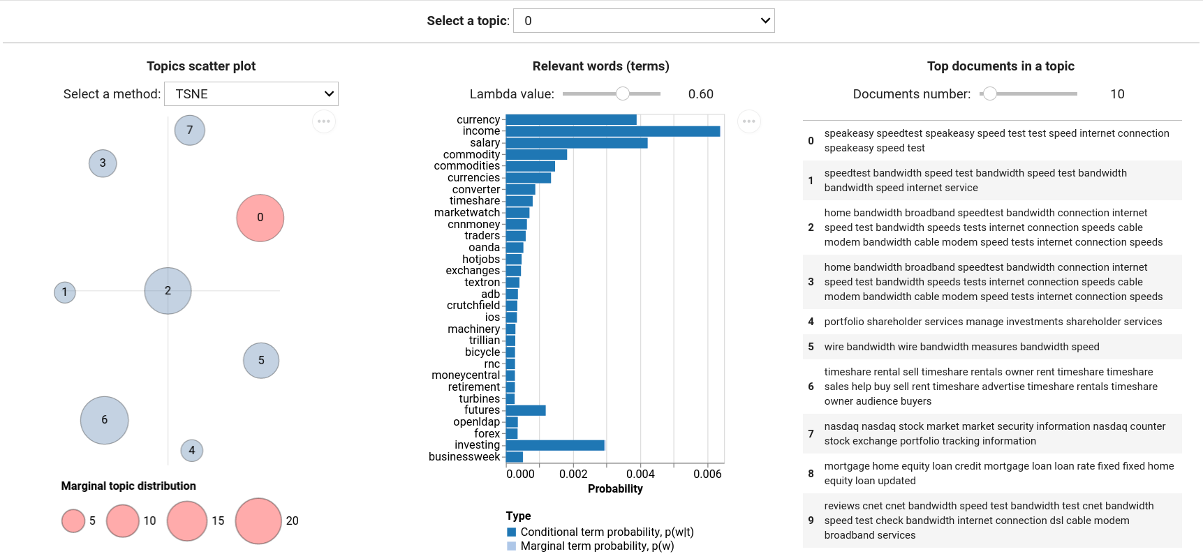
+**tmplot** is a comprehensive Python package for **topic modeling analysis and visualization**. Built for data scientists and researchers, it provides powerful interactive reports and advanced analytics that extend beyond traditional LDAvis/pyLDAvis capabilities.
+
+**Analyze** • **Visualize** • **Compare** multiple topic models with ease
 
 ![Plots](https://raw.githubusercontent.com/maximtrp/tmplot/main/images/topics_terms_plots.png)
 
-## Features
+## Key Features
+
+### Interactive Visualization
+
+- **Topic scatter plots** with customizable coordinates and sizing
+- **Term probability charts** with relevance weighting
+- **Document analysis** showing top documents per topic
+- **Interactive reports** with real-time parameter adjustment
+
+### Advanced Analytics
 
-- Supported models:
+- **Topic stability analysis** across multiple model runs
+- **Model comparison** with sophisticated distance metrics
+- **Saliency calculations** for term importance
+- **Entropy metrics** for model optimization
 
-  - [tomotopy](https://bab2min.github.io/tomotopy/): `LDAModel`, `LLDAModel`, `CTModel`, `DMRModel`, `HDPModel`, `PTModel`, `SLDAModel`, `GDMRModel`
-  - [gensim](https://radimrehurek.com/gensim/): `LdaModel`, `LdaMulticore`
-  - [bitermplus](https://github.com/maximtrp/bitermplus): `BTM`
+### Model Support
 
-- Supported distance metrics:
+- **[tomotopy](https://bab2min.github.io/tomotopy/)**: `LDAModel`, `LLDAModel`, `CTModel`, `DMRModel`, `HDPModel`, `PTModel`, `SLDAModel`, `GDMRModel`
+- **[gensim](https://radimrehurek.com/gensim/)**: `LdaModel`, `LdaMulticore`
+- **[bitermplus](https://github.com/maximtrp/bitermplus)**: `BTM`
 
-  - Kullback-Leibler (symmetric and non-symmetric) divergence
-  - Jenson-Shannon divergence
-  - Jeffrey's divergence
-  - Hellinger distance
-  - Bhattacharyya distance
-  - Total variation distance
-  - Jaccard inversed index
+### Distance Metrics
 
-- Supported [algorithms](https://scikit-learn.org/stable/modules/classes.html#module-sklearn.manifold) for calculating topics scatter coordinates:
+- Kullback-Leibler (symmetric & non-symmetric)
+- Jensen-Shannon divergence
+- Jeffrey's divergence
+- Hellinger & Bhattacharyya distances
+- Total variation distance
+- Jaccard index
 
-  - t-SNE
-  - SpectralEmbedding
-  - MDS
-  - LocallyLinearEmbedding
-  - Isomap
+### Dimensionality Reduction
+
+t-SNE, SpectralEmbedding, MDS, LocallyLinearEmbedding, Isomap
 
 ## Donate
 
@@ -102,55 +114,77 @@ If you find this package useful, please consider donating any amount of money. T
 
 <a href="https://www.buymeacoffee.com/maximtrp" target="_blank"><img src="https://cdn.buymeacoffee.com/buttons/v2/default-yellow.png" alt="Buy Me A Coffee" style="height: 60px !important;width: 217px !important;" ></a>
 
-## Installation
+## Quick Start
 
-The package can be installed from PyPi:
+### Installation
 
 ```bash
+# From PyPI (recommended)
 pip install tmplot
-```
-
-Or directly from this repository:
 
-```bash
+# Development version
 pip install git+https://github.com/maximtrp/tmplot.git
 ```
 
-## Dependencies
+### Basic Usage
+
+```python
+import tmplot as tmp
+
+# Load your topic model and documents
+model = your_fitted_model  # tomotopy, gensim, or bitermplus
+docs = your_documents
 
-- `numpy`
-- `scipy`
-- `scikit-learn`
-- `pandas`
-- `altair`
-- `ipywidgets`
-- `tomotopy`, `gensim`, and `bitermplus` (optional)
+# Create interactive report
+tmp.report(model, docs=docs)
 
-## Quick example
+# Or create individual visualizations
+coords = tmp.prepare_coords(model)
+tmp.plot_scatter_topics(coords, size_col='size')
+```
+
+## Advanced Examples
+
+### Get Stable Topics
 
 ```python
-# Importing packages
 import tmplot as tmp
-import pickle as pkl
-import pandas as pd
 
-# Reading a model from a file
-with open('data/model.pkl', 'rb') as file:
-    model = pkl.load(file)
+# Find stable topics across multiple models
+models = [model1, model2, model3, model4]
+closest_topics, distances = tmp.get_closest_topics(models)
+stable_topics, stable_distances = tmp.get_stable_topics(closest_topics, distances)
+```
+
+### Analyze Model
+
+```python
+# Calculate entropy for model selection
+entropy_score = tmp.entropy(phi_matrix)
 
-# Reading documents from a file
-docs = pd.read_csv('data/docs.txt.gz', header=None).values.ravel()
+# Analyze topic stability
+saliency = tmp.get_salient_terms(phi, theta)
+```
 
-# Plotting topics as a scatter plot
-topics_coords = tmp.prepare_coords(model)
-tmp.plot_scatter_topics(topics_coords, size_col='size', label_col='label')
+### Visualize
 
-# Plotting terms probabilities
-terms_probs = tmp.calc_terms_probs_ratio(phi, topic=0, lambda_=1)
-tmp.plot_terms(terms_probs)
+```python
+# Create topic distance matrix with different metrics
+topic_dists = tmp.get_topics_dist(phi, method='jensen-shannon')
 
-# Running report interface
-tmp.report(model, docs=docs, width=250)
+# Generate coordinates with custom algorithm
+coords = tmp.get_topics_scatter(topic_dists, theta, method='tsne')
+tmp.plot_scatter_topics(coords, topic=3)  # Highlight topic 3
 ```
 
-You can find more examples in the [tutorial](https://tmplot.readthedocs.io/en/latest/tutorial.html).
+## Documentation & Examples
+
+- [Complete Tutorial](https://tmplot.readthedocs.io/en/latest/tutorial.html) - Step-by-step guide
+- [API Reference](https://tmplot.readthedocs.io/) - Full documentation
+- [Example Notebooks](https://github.com/maximtrp/tmplot/tree/main/examples) - Jupyter examples
+
+## Requirements
+
+**Core dependencies:** `numpy`, `scipy`, `scikit-learn`, `pandas`, `altair`, `ipywidgets`
+
+**Optional models:** `tomotopy`, `gensim`, `bitermplus`

tmplot-0.3.0/README.md

@@ -0,0 +1,131 @@
+# tmplot
+
+[![Codacy coverage](https://img.shields.io/codacy/coverage/5939b1cf99bc4f9d91de11c0d3ff9e50)](https://app.codacy.com/gh/maximtrp/tmplot/coverage)
+[![Codacy grade](https://img.shields.io/codacy/grade/5939b1cf99bc4f9d91de11c0d3ff9e50)](https://app.codacy.com/gh/maximtrp/tmplot)
+[![GitHub Workflow Status](https://img.shields.io/github/actions/workflow/status/maximtrp/tmplot/python-package.yml?label=tests)](https://github.com/maximtrp/tmplot/actions/workflows/python-package.yml)
+[![Documentation Status](https://readthedocs.org/projects/tmplot/badge/?version=latest)](https://tmplot.readthedocs.io/en/latest/?badge=latest)
+[![Downloads](https://static.pepy.tech/badge/tmplot)](https://pepy.tech/project/tmplot)
+[![PyPI](https://img.shields.io/pypi/v/tmplot)](https://pypi.org/project/tmplot)
+[![Issues](https://img.shields.io/github/issues/maximtrp/tmplot.svg)](https://github.com/maximtrp/tmplot/issues)
+
+**tmplot** is a comprehensive Python package for **topic modeling analysis and visualization**. Built for data scientists and researchers, it provides powerful interactive reports and advanced analytics that extend beyond traditional LDAvis/pyLDAvis capabilities.
+
+**Analyze** • **Visualize** • **Compare** multiple topic models with ease
+
+![Plots](https://raw.githubusercontent.com/maximtrp/tmplot/main/images/topics_terms_plots.png)
+
+## Key Features
+
+### Interactive Visualization
+
+- **Topic scatter plots** with customizable coordinates and sizing
+- **Term probability charts** with relevance weighting
+- **Document analysis** showing top documents per topic
+- **Interactive reports** with real-time parameter adjustment
+
+### Advanced Analytics
+
+- **Topic stability analysis** across multiple model runs
+- **Model comparison** with sophisticated distance metrics
+- **Saliency calculations** for term importance
+- **Entropy metrics** for model optimization
+
+### Model Support
+
+- **[tomotopy](https://bab2min.github.io/tomotopy/)**: `LDAModel`, `LLDAModel`, `CTModel`, `DMRModel`, `HDPModel`, `PTModel`, `SLDAModel`, `GDMRModel`
+- **[gensim](https://radimrehurek.com/gensim/)**: `LdaModel`, `LdaMulticore`
+- **[bitermplus](https://github.com/maximtrp/bitermplus)**: `BTM`
+
+### Distance Metrics
+
+- Kullback-Leibler (symmetric & non-symmetric)
+- Jensen-Shannon divergence
+- Jeffrey's divergence
+- Hellinger & Bhattacharyya distances
+- Total variation distance
+- Jaccard index
+
+### Dimensionality Reduction
+
+t-SNE, SpectralEmbedding, MDS, LocallyLinearEmbedding, Isomap
+
+## Donate
+
+If you find this package useful, please consider donating any amount of money. This will help me spend more time on supporting open-source software.
+
+<a href="https://www.buymeacoffee.com/maximtrp" target="_blank"><img src="https://cdn.buymeacoffee.com/buttons/v2/default-yellow.png" alt="Buy Me A Coffee" style="height: 60px !important;width: 217px !important;" ></a>
+
+## Quick Start
+
+### Installation
+
+```bash
+# From PyPI (recommended)
+pip install tmplot
+
+# Development version
+pip install git+https://github.com/maximtrp/tmplot.git
+```
+
+### Basic Usage
+
+```python
+import tmplot as tmp
+
+# Load your topic model and documents
+model = your_fitted_model  # tomotopy, gensim, or bitermplus
+docs = your_documents
+
+# Create interactive report
+tmp.report(model, docs=docs)
+
+# Or create individual visualizations
+coords = tmp.prepare_coords(model)
+tmp.plot_scatter_topics(coords, size_col='size')
+```
+
+## Advanced Examples
+
+### Get Stable Topics
+
+```python
+import tmplot as tmp
+
+# Find stable topics across multiple models
+models = [model1, model2, model3, model4]
+closest_topics, distances = tmp.get_closest_topics(models)
+stable_topics, stable_distances = tmp.get_stable_topics(closest_topics, distances)
+```
+
+### Analyze Model
+
+```python
+# Calculate entropy for model selection
+entropy_score = tmp.entropy(phi_matrix)
+
+# Analyze topic stability
+saliency = tmp.get_salient_terms(phi, theta)
+```
+
+### Visualize
+
+```python
+# Create topic distance matrix with different metrics
+topic_dists = tmp.get_topics_dist(phi, method='jensen-shannon')
+
+# Generate coordinates with custom algorithm
+coords = tmp.get_topics_scatter(topic_dists, theta, method='tsne')
+tmp.plot_scatter_topics(coords, topic=3)  # Highlight topic 3
+```
+
+## Documentation & Examples
+
+- [Complete Tutorial](https://tmplot.readthedocs.io/en/latest/tutorial.html) - Step-by-step guide
+- [API Reference](https://tmplot.readthedocs.io/) - Full documentation
+- [Example Notebooks](https://github.com/maximtrp/tmplot/tree/main/examples) - Jupyter examples
+
+## Requirements
+
+**Core dependencies:** `numpy`, `scipy`, `scikit-learn`, `pandas`, `altair`, `ipywidgets`
+
+**Optional models:** `tomotopy`, `gensim`, `bitermplus`

{tmplot-0.1.3 → tmplot-0.3.0}/src/tmplot/__init__.py

@@ -5,4 +5,4 @@ from ._stability import *  # noqa: F401, F403
 from ._vis import *  # noqa: F401, F403
 from ._metrics import *  # noqa: F401, F403
 
-__version__ = '0.1.3'
+__version__ = "0.3.0"

{tmplot-0.1.3 → tmplot-0.3.0}/src/tmplot/_distance.py

@@ -1,13 +1,17 @@
-__all__ = [
-    'get_topics_dist', 'get_topics_scatter', 'get_top_topic_words']
-from typing import Union, List
+__all__ = ["get_topics_dist", "get_topics_scatter", "get_top_topic_words"]
+from typing import Optional, Union, List
 from itertools import combinations
-from pandas import DataFrame
+from pandas import DataFrame, Index
 import numpy as np
 from scipy.special import kl_div
 from scipy.spatial import distance
 from sklearn.manifold import (
-    TSNE, Isomap, LocallyLinearEmbedding, MDS, SpectralEmbedding)
+    TSNE,
+    Isomap,
+    LocallyLinearEmbedding,
+    MDS,
+    SpectralEmbedding,
+)
 from ._helpers import calc_topics_marg_probs
 
 
@@ -17,32 +21,38 @@ def _dist_klb(a1: np.ndarray, a2: np.ndarray):
 
 
 def _dist_sklb(a1: np.ndarray, a2: np.ndarray):
-    dist = kl_div(a1, a2) + kl_div(a1, a2)
+    dist = kl_div(a1, a2) + kl_div(a2, a1)
     return dist[np.isfinite(dist)].sum()
 
 
 def _dist_jsd(a1: np.ndarray, a2: np.ndarray):
-    dist = 0.5 * kl_div(a1, a2) + 0.5 * kl_div(a1, a2)
+    m = 0.5 * (a1 + a2)
+    dist = 0.5 * kl_div(a1, m) + 0.5 * kl_div(a2, m)
     return dist[np.isfinite(dist)].sum()
 
 
 def _dist_jef(a1: np.ndarray, a2: np.ndarray):
     vals = (a1 - a2) * (np.log(a1) - np.log(a2))
-    vals[(vals <= 0) | ~np.isfinite(vals)] = 0.
+    vals[(vals <= 0) | ~np.isfinite(vals)] = 0.0
     return vals.sum()
 
 
+# Small value for numerical stability
+EPSILON = 1e-64
+
+
 def _dist_hel(a1: np.ndarray, a2: np.ndarray):
-    a1[(a1 <= 0) | ~np.isfinite(a1)] = 1e-64
-    a2[(a2 <= 0) | ~np.isfinite(a2)] = 1e-64
-    hel_val = distance.euclidean(
-        np.sqrt(a1), np.sqrt(a2)) / np.sqrt(2)
+    a1_safe = a1.copy()
+    a2_safe = a2.copy()
+    a1_safe[(a1_safe <= 0) | ~np.isfinite(a1_safe)] = EPSILON
+    a2_safe[(a2_safe <= 0) | ~np.isfinite(a2_safe)] = EPSILON
+    hel_val = distance.euclidean(np.sqrt(a1_safe), np.sqrt(a2_safe)) / np.sqrt(2)
     return hel_val
 
 
 def _dist_bhat(a1: np.ndarray, a2: np.ndarray):
     pq = a1 * a2
-    pq[(pq <= 0) | ~np.isfinite(pq)] = 1e-64
+    pq[(pq <= 0) | ~np.isfinite(pq)] = EPSILON
     dist = -np.log(np.sum(np.sqrt(pq)))
     return dist
 
@@ -52,9 +62,9 @@ def _dist_tv(a1: np.ndarray, a2: np.ndarray):
     return dist
 
 
-def _dist_jac(a1: np.ndarray, a2: np.ndarray,  top_words=100):
-    a = np.argsort(a1)[:-top_words-1:-1]
-    b = np.argsort(a2)[:-top_words-1:-1]
+def _dist_jac(a1: np.ndarray, a2: np.ndarray, top_words=100):
+    a = np.argsort(a1)[: -top_words - 1 : -1]
+    b = np.argsort(a2)[: -top_words - 1 : -1]
     j_num = np.intersect1d(a, b, assume_unique=False).size
     j_den = np.union1d(a, b).size
     jac_val = 1 - j_num / j_den
@@ -62,9 +72,8 @@ def _dist_jac(a1: np.ndarray, a2: np.ndarray,  top_words=100):
 
 
 def get_topics_dist(
-        phi: Union[np.ndarray, DataFrame],
-        method: str = "sklb",
-        **kwargs) -> np.ndarray:
+    phi: Union[np.ndarray, DataFrame], method: str = "sklb", **kwargs
+) -> np.ndarray:
     """Finding closest topics in models.
 
     Parameters
@@ -90,6 +99,14 @@ def get_topics_dist(
         Topics distances matrix.
     """
     phi_copy = np.array(phi)
+
+    if phi_copy.ndim != 2:
+        raise ValueError("phi must be a 2D array (words x topics)")
+    if np.any(phi_copy < 0):
+        raise ValueError("phi must contain non-negative probability values")
+    if not np.allclose(phi_copy.sum(axis=0), 1.0, atol=1e-6):
+        raise ValueError("phi columns must sum to 1 (probability distributions)")
+
     topics_num = phi_copy.shape[1]
     topics_pairs = combinations(range(topics_num), 2)
 
@@ -110,16 +127,18 @@ def get_topics_dist(
     for i, j in topics_pairs:
         _dist_func = dist_funcs.get(method, "sklb")
         topics_dists[((i, j), (j, i))] = _dist_func(
-            phi_copy[:, i], phi_copy[:, j], **kwargs)
+            phi_copy[:, i], phi_copy[:, j], **kwargs
+        )
 
     return topics_dists
 
 
 def get_topics_scatter(
-        topic_dists: np.ndarray,
-        theta: np.ndarray,
-        method: str = 'tsne',
-        method_kws: dict = None) -> DataFrame:
+    topic_dists: np.ndarray,
+    theta: np.ndarray,
+    method: str = "tsne",
+    method_kws: Optional[dict] = None,
+) -> DataFrame:
     """Calculate topics coordinates for a scatter plot.
 
     Parameters
@@ -146,52 +165,53 @@ def get_topics_scatter(
         Topics scatter coordinates.
     """
     if not method_kws:
-        method_kws = {'n_components': 2}
+        method_kws = {"n_components": 2}
 
-    if method == 'tsne':
-        method_kws.setdefault('init', 'pca')
-        method_kws.setdefault('learning_rate', 'auto')
-        method_kws.setdefault(
-            'perplexity', min(50, max(topic_dists.shape[0] // 2, 1)))
+    if method == "tsne":
+        method_kws.setdefault("init", "pca")
+        method_kws.setdefault("learning_rate", "auto")
+        method_kws.setdefault("perplexity", min(50, max(topic_dists.shape[0] // 2, 1)))
         transformer = TSNE(**method_kws)
 
-    elif method == 'sem':
-        method_kws.setdefault('affinity', 'precomputed')
+    elif method == "sem":
+        method_kws.setdefault("affinity", "precomputed")
         transformer = SpectralEmbedding(**method_kws)
 
-    elif method == 'mds':
-        method_kws.setdefault('dissimilarity', 'precomputed')
-        method_kws.setdefault('normalized_stress', 'auto')
+    elif method == "mds":
+        method_kws.setdefault("dissimilarity", "precomputed")
+        method_kws.setdefault("normalized_stress", "auto")
+        method_kws.setdefault("n_init", 1)
         transformer = MDS(**method_kws)
 
-    elif method == 'lle':
-        method_kws['method'] = 'standard'
+    elif method == "lle":
+        method_kws["method"] = "standard"
         transformer = LocallyLinearEmbedding(**method_kws)
 
-    elif method == 'ltsa':
-        method_kws['method'] = 'ltsa'
+    elif method == "ltsa":
+        method_kws["method"] = "ltsa"
         transformer = LocallyLinearEmbedding(**method_kws)
 
-    elif method == 'isomap':
+    elif method == "isomap":
         transformer = Isomap(**method_kws)
 
     coords = transformer.fit_transform(topic_dists)
 
-    topics_xy = DataFrame(coords, columns=['x', 'y'])
-    topics_xy['topic'] = topics_xy.index.astype(int)
-    topics_xy['size'] = calc_topics_marg_probs(theta)
-    size_sum = topics_xy['size'].sum()
+    topics_xy = DataFrame(coords, columns=Index(["x", "y"]))
+    topics_xy["topic"] = topics_xy.index.astype(int)
+    topics_xy["size"] = calc_topics_marg_probs(theta)
+    size_sum = topics_xy["size"].sum()
     if size_sum > 0:
-        topics_xy['size'] *= (100 / topics_xy['size'].sum())
+        topics_xy["size"] *= 100 / topics_xy["size"].sum()
     else:
-        topics_xy['size'] = np.nan
+        topics_xy["size"] = np.nan
     return topics_xy
 
 
 def get_top_topic_words(
-        phi: DataFrame,
-        words_num: int = 20,
-        topics_idx: Union[List[int], np.ndarray] = None) -> DataFrame:
+    phi: DataFrame,
+    words_num: int = 20,
+    topics_idx: Optional[Union[List[int], np.ndarray]] = None,
+) -> DataFrame:
     """Select top topic words from a fitted model.
 
     Parameters
@@ -209,9 +229,6 @@ def get_top_topic_words(
     DataFrame
         Words with highest probabilities in all (or selected) topics.
     """
-    return phi.loc[:, topics_idx or phi.columns]\
-        .apply(
-            lambda x: x
-            .sort_values(ascending=False)
-            .head(words_num).index, axis=0
+    return phi.loc[:, topics_idx or phi.columns].apply(
+        lambda x: x.sort_values(ascending=False).head(words_num).index, axis=0
     )