pyatoms-spm 1.0.0__tar.gz
This diff represents the content of publicly available package versions that have been released to one of the supported registries. The information contained in this diff is provided for informational purposes only and reflects changes between package versions as they appear in their respective public registries.
- pyatoms_spm-1.0.0/PKG-INFO +354 -0
- pyatoms_spm-1.0.0/README.md +337 -0
- pyatoms_spm-1.0.0/pyatoms/PyAtoms_GUI.py +364 -0
- pyatoms_spm-1.0.0/pyatoms/PyAtoms_Widgets.py +5408 -0
- pyatoms_spm-1.0.0/pyatoms/__init__.py +0 -0
- pyatoms_spm-1.0.0/pyatoms/hexatoms.py +183 -0
- pyatoms_spm-1.0.0/pyatoms/logo_magma_Small.png +0 -0
- pyatoms_spm-1.0.0/pyatoms/moirelattice.py +376 -0
- pyatoms_spm-1.0.0/pyatoms/squareatoms.py +140 -0
- pyatoms_spm-1.0.0/pyatoms/stripes.py +113 -0
- pyatoms_spm-1.0.0/pyatoms_spm.egg-info/PKG-INFO +354 -0
- pyatoms_spm-1.0.0/pyatoms_spm.egg-info/SOURCES.txt +16 -0
- pyatoms_spm-1.0.0/pyatoms_spm.egg-info/dependency_links.txt +1 -0
- pyatoms_spm-1.0.0/pyatoms_spm.egg-info/entry_points.txt +2 -0
- pyatoms_spm-1.0.0/pyatoms_spm.egg-info/requires.txt +5 -0
- pyatoms_spm-1.0.0/pyatoms_spm.egg-info/top_level.txt +1 -0
- pyatoms_spm-1.0.0/pyproject.toml +36 -0
- pyatoms_spm-1.0.0/setup.cfg +4 -0
|
@@ -0,0 +1,354 @@
|
|
|
1
|
+
Metadata-Version: 2.4
|
|
2
|
+
Name: pyatoms-spm
|
|
3
|
+
Version: 1.0.0
|
|
4
|
+
Summary: A graphical simulator for scanning probe microscopy images and atomic lattices.
|
|
5
|
+
Author: Asari G. Prado
|
|
6
|
+
Author-email: Christopher Gutiérrez <gutierrez@physics.ucla.edu>, Jacob González <jg.cobi12@gmail.com>
|
|
7
|
+
Project-URL: Homepage, https://github.com/GutierrezPhys/PyAtoms
|
|
8
|
+
Project-URL: Repository, https://github.com/GutierrezPhys/PyAtoms
|
|
9
|
+
Project-URL: Issues, https://github.com/GutierrezPhys/PyAtoms
|
|
10
|
+
Requires-Python: >=3.10
|
|
11
|
+
Description-Content-Type: text/markdown
|
|
12
|
+
Requires-Dist: numpy
|
|
13
|
+
Requires-Dist: scipy
|
|
14
|
+
Requires-Dist: matplotlib
|
|
15
|
+
Requires-Dist: QtPy
|
|
16
|
+
Requires-Dist: PyQt6
|
|
17
|
+
|
|
18
|
+
# PyAtoms
|
|
19
|
+
|
|
20
|
+
|
|
21
|
+
Simulates scanning probe microscopy (SPM) images. Please read our preprint describing PyAtoms: <a href="https://arxiv.org/abs/2412.18332" target="__blank" rel="noopener noreferrer"> https://arxiv.org/abs/2412.18332. </a>
|
|
22
|
+
|
|
23
|
+
(Formerly named: SPM Simulator, Atom Simulator)
|
|
24
|
+
|
|
25
|
+
|
|
26
|
+

|
|
27
|
+
|
|
28
|
+
|
|
29
|
+
### Dependencies:
|
|
30
|
+
- Python 3.0 or newer
|
|
31
|
+
- NumPy
|
|
32
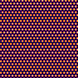
|
+
- Matplotlib
|
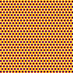
|
33
|
+
- SciPy
|
|
34
|
+
- QtPy
|
|
35
|
+
- PyQt5 or PyQt6
|
|
36
|
+
|
|
37
|
+
PyAtoms is compatible with both PyQt5 and PyQt6 through QtPy. PyQt6 is installed by default when PyAtoms is installed using pip.
|
|
38
|
+
|
|
39
|
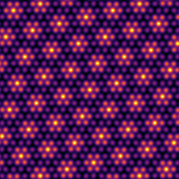
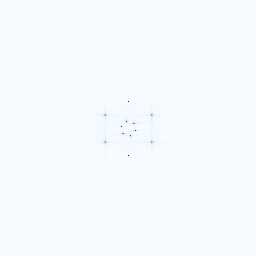
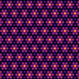
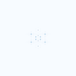
+
## Installation instructions - macOS and WIndows
|
|
40
|
+
|
|
41
|
+
### Install with pip
|
|
42
|
+
|
|
43
|
+
PyAtoms can be installed using pip:
|
|
44
|
+
|
|
45
|
+
```bash
|
|
46
|
+
pip install pyatoms-spm
|
|
47
|
+
```
|
|
48
|
+
|
|
49
|
+
After installation, launch PyAtoms by typing:
|
|
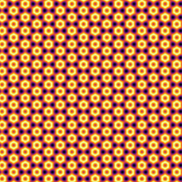
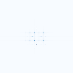
50
|
+
|
|
51
|
+
```bash
|
|
52
|
+
pyatoms
|
|
53
|
+
```
|
|
54
|
+
|
|
55
|
+
### Run from source
|
|
56
|
+
|
|
57
|
+
PyAtoms can also be run directly from the source code.
|
|
58
|
+
|
|
59
|
+
1. Click the green **Code** button at the top of this GitHub page and select **Download ZIP**.
|
|
60
|
+
|
|
61
|
+
2. Extract the downloaded ZIP file.
|
|
62
|
+
|
|
63
|
+
3. Open a terminal or command line:
|
|
64
|
+
- **Windows:** open Command Prompt, PowerShell, or the Anaconda Prompt.
|
|
65
|
+
- **macOS:** open the Terminal application.
|
|
66
|
+
|
|
67
|
+
4. In the terminal, navigate to the extracted PyAtoms folder.
|
|
68
|
+
|
|
69
|
+
If the ZIP was extracted into your Downloads folder, you can usually use:
|
|
70
|
+
|
|
71
|
+
**Windows Command Prompt:**
|
|
72
|
+
|
|
73
|
+
```bash
|
|
74
|
+
cd %USERPROFILE%\Downloads\PyAtoms-main
|
|
75
|
+
```
|
|
76
|
+
|
|
77
|
+
**Wndows PowerShell:**
|
|
78
|
+
|
|
79
|
+
```powershell
|
|
80
|
+
cd "$HOME\Downloads\PyAtoms-main"
|
|
81
|
+
```
|
|
82
|
+
|
|
83
|
+
**macOS:**
|
|
84
|
+
|
|
85
|
+
```bash
|
|
86
|
+
cd ~/Downloads/PyAtoms-main
|
|
87
|
+
```
|
|
88
|
+
|
|
89
|
+
If you extracted the folder somewhere else, replace the path above with the location of your extracted PyAtoms folder.
|
|
90
|
+
|
|
91
|
+
5. Install the required Python packages.
|
|
92
|
+
|
|
93
|
+
For PyQt6:
|
|
94
|
+
|
|
95
|
+
```bash
|
|
96
|
+
python -m pip install numpy scipy matplotlib QtPy PyQt6
|
|
97
|
+
```
|
|
98
|
+
|
|
99
|
+
Or, if you use PyQt5:
|
|
100
|
+
|
|
101
|
+
```bash
|
|
102
|
+
python -m pip install numpy scipy matplotlib QtPy PyQt5
|
|
103
|
+
```
|
|
104
|
+
|
|
105
|
+
6. From inside the extracted PyAtoms folder, start PyAtoms with:
|
|
106
|
+
|
|
107
|
+
```bash
|
|
108
|
+
python -m pyatoms.PyAtoms_GUI
|
|
109
|
+
```
|
|
110
|
+
|
|
111
|
+
PyAtoms is compatile with both PyQt5 and PyQt6 through QtPy.
|
|
112
|
+
|
|
113
|
+
## Known issues
|
|
114
|
+
|
|
115
|
+
02-Sep-2026: Pyatoms is compatile with both PyQt5 and PyQt6 through QtPy. PyQt6 is installed by default when installing PyAtoms through pip.
|
|
116
|
+
|
|
117
|
+
06-Nov-2025: PyAtoms is currently **not** compatible with PyQt 6. Still compatible with latest PyQt5 (5.15.11)
|
|
118
|
+
|
|
119
|
+
28-Oct-2024: No known issues. Works correctly with latest version of Matplotlib (3.9.2)
|
|
120
|
+
|
|
121
|
+
### For windows users:
|
|
122
|
+
- Make sure python is installed and that its path is set in your environment
|
|
123
|
+
- To check if it is, open the command line and type
|
|
124
|
+
```
|
|
125
|
+
python -V
|
|
126
|
+
```
|
|
127
|
+
- Alternatively, if you installed python, NumPy, SciPy, etc. through Anaconda for Windows, you can run the above code through the Anaconda prompt.
|
|
128
|
+
|
|
129
|
+
For any other issues or crash reports, suggestions, contact gutierrez@physics.ucla.edu
|
|
130
|
+
|
|
131
|
+
##
|
|
132
|
+
## How to use
|
|
133
|
+
|
|
134
|
+

|
|
135
|
+
|
|
136
|
+
|
|
137
|
+
Note that all fields accept typical mathematical operations in python and NumPy such as `+` `-` `*` `/` `sqrt` `log` and all valid NumPy functions `func` can be called via `np.func()`.
|
|
138
|
+
|
|
139
|
+
1. **Number of lattices** (moiré, CDW, superlattice) and **Moiré model** (Simple, Log)
|
|
140
|
+
- Choose to simulate a 1, 2 or 3 layer lattice
|
|
141
|
+
- Lattice 1 parameters change the single/first layer.
|
|
142
|
+
- Lattice 2 only works if bilayer/trilayer are selected. These change the second lattice.
|
|
143
|
+
- Lattice 3 only works if trilayer is selected. These change the third lattice.
|
|
144
|
+
- Choose the model to simulate the moiré/CDW/superlattice
|
|
145
|
+
- `Simple`: This minimal toy model approximates the moiré image, $T_M$, as the weighted sum between the sum of the individual lattices, $\sum_l Z_l$, and the product of the lattices, $\prod_l Z_l$ and is given by $T_M \propto (1-\eta)\sum_l Z_l + \eta\prod_L Z_l$. This toy model provides a good match to experimental STM images and offers a wide image contrast. However, the Fourier transforms -- by design -- contains only the first order atomic Bragg and moiré lattice peaks. The image is normalized such that $0\leq T_M \leq 1$.
|
|
146
|
+
- `eta`, $\eta$ : A phenomenological parameter we use to weigh the relative strength of the sum of lattices, $\sum_l Z_l$, to the product of lattices, $\prod_L Z_l$. $\eta$ is a real number between 0 and 1: The moiré/superlattice image for $\eta=0$ purely the sum and $\eta=1$ is purely the product.
|
|
147
|
+
- `Log`: This model, described by Joucken *et al* (<a href="https://doi.org/10.1016/j.carbon.2014.11.030" target="_blank" rel="noopener noreferrer"> *Carbon* **83**, 48 (2015). </a>) is rooted in the constant-current tunneling process and takes into account the distance of the multilayers to the STM tip. The moiré/superlattice image, $T_M^L$, is approximated as $T_M^L \propto \ln|Z_1 + Z_2 e^{-\xi}|$ (bilayer) or $T_M^L \propto \ln|Z_1 + Z_2 e^{-\xi} + Z_3 e^{-2\xi}|$ (trilayer). This model provides a good match to both experimental STM images and their Fourier transforms, at the cost of limited image contrast.
|
|
148
|
+
- `xi`, $\xi$ : The ratio of the inter-layer distance, $d$, and out-of-plane wavefunction decay length, $\lambda$: $\xi = d/\lambda$. $\xi$ is a real number between 0 and 10: For $\xi=0$, the intensity of the lattices is maximized; for $\xi$ = 10, only the top lattice, $Z_1$, is imaged.
|
|
149
|
+
|
|
150
|
+
2. Image parameters
|
|
151
|
+
- `Real resolution`: Current spatial resolution, defined as L/pix, in units of nm/pix.
|
|
152
|
+
- `K-space resolution`: Current spatial resolution in reciprocal space, defined as 2π/L, in units of nm⁻¹/pix.
|
|
153
|
+
- `Pixels`: number of pixels. Must be an integer or a mathematical expression of integers.
|
|
154
|
+
- `Image length, L`: length of the image window in nanometers. Must be a real number or a mathematical expression of real numbers.
|
|
155
|
+
- `Scan angle, θ`: Rotation (counter-clockwise) of the atomic lattice. Must be a real number or a mathematical expression of real numbers.
|
|
156
|
+
- `Image offset`: Location of center of image. Must be a pair of real numbers, or a mathematical expression of real numbers, separated by a comma, e.g. -1.2,4.5.
|
|
157
|
+
|
|
158
|
+
3. Colormap
|
|
159
|
+
- `Real space image`: colormap of the real space simulated atomic lattice.
|
|
160
|
+
- `FFT`: colormap of the 2D fast Fourier transform.
|
|
161
|
+
|
|
162
|
+
4. Low pass filtering
|
|
163
|
+
- `Gaussian width, σ`: radius of a Gaussian mask in real space in units of pixels. The half-width at half-max of the gaussian is shown as a white circle in the bottom left corner of the image.
|
|
164
|
+
- The radius of the gaussian mask in nanometers is shown in the text box.
|
|
165
|
+
|
|
166
|
+
5. Save files
|
|
167
|
+
- Click to save the files to a specific directory.
|
|
168
|
+
- Clicking will open the file explorer.
|
|
169
|
+
- Navigate to the directory you want to save the files in
|
|
170
|
+
- Input a `filename` to save as
|
|
171
|
+
- It will save a folder called `filename` with 4 files:
|
|
172
|
+
- .png images of the real space and FFT, .txt file of the real space image, .txt file of the parameter values
|
|
173
|
+
- `filename.png`, `filename_FFT.png`, `filename.txt`, `filename_params.txt`
|
|
174
|
+
- Example of folder with saved files:
|
|
175
|
+
|
|
176
|
+
<img width="700" alt="Screen Shot 2022-08-04 at 1 30 29 PM" src="https://user-images.githubusercontent.com/62832051/182946811-ba2a1e4d-04d7-4658-b013-38dac1c8ef42.png">
|
|
177
|
+
- Example of params .txt file:
|
|
178
|
+
|
|
179
|
+
<img width="446" alt="Screen Shot 2022-08-03 at 3 40 46 PM" src="https://user-images.githubusercontent.com/62832051/182724722-b820f3b3-a2e2-413c-8c9d-cb03da7b78ce.png">
|
|
180
|
+
|
|
181
|
+
|
|
182
|
+
6. SPM image time estimator
|
|
183
|
+
- `Tip velocity`: Velocity of the tip, $v_t$ across 1 line in nanometers/second. The total image time is calculated by considering the total pixels, scanning left/right and in a single slow-scan direction (upwards, for example). This time is estimated via $T_{im} = (2 * N_{pix} * L) / v_t$, where $N_{pix}$ is the number of pixels in the image, $L$ is the length of the image in nanometers, and the factor 2 takes into account the left/right fast-scan direction.
|
|
184
|
+
|
|
185
|
+
7. Spectroscopy map Time estimator
|
|
186
|
+
- `Time per spectra`: Total time in seconds (including overhead) to record a single spectrum, $T_{spec}$ i.e. one dI/dV(V) sweep. We assume that spectra are recorded in one direction along both the fast- and slow-scan direction. The time is estimated via $T_{map} = N_{pix}^2 * T_{spec} + (2 * N_{pix} * L) / v_t$.
|
|
187
|
+
|
|
188
|
+
8. Lattices
|
|
189
|
+
- Parameters tab
|
|
190
|
+
- `symmetry`: Choose to simulate either a triangular/hexagonal or square lattice.
|
|
191
|
+
- `Lattice constant`: periodicity/spacing between atoms in nanometers.
|
|
192
|
+
- `Twist angle`: twists the second lattice with respect to the first lattice (in Lattice 2 params) // twists the third lattice with respect to the second lattice (in Lattice 3 params)
|
|
193
|
+
|
|
194
|
+
- Sublattices tab -- only affects hexagonal (triangular/honeycomb) lattices
|
|
195
|
+
- Lattice site at the image `origin`: choose whether the `origin` should be a hollow site, an A-site atom or a B-site atom
|
|
196
|
+
- To test this, set `L = 1` and click the different options for the origin
|
|
197
|
+
<img width="400" alt="Screen Shot 2022-10-03 at 4 26 18 PM" src="https://user-images.githubusercontent.com/62832051/193703355-855b46de-f020-428f-af81-0ae4fee0bf57.png">
|
|
198
|
+
|
|
199
|
+
|
|
200
|
+
- Weight of sublattices:
|
|
201
|
+
- `alpha1`, $\alpha_1$ : weight of A sublattice
|
|
202
|
+
- `beta1`, $\beta_1$: weight of B sublattice
|
|
203
|
+
- For a triangular lattice: `alpha = 1`, `beta = 0`
|
|
204
|
+
|
|
205
|
+
|
|
206
|
+
|
|
207
|
+
- For a honeycomb lattice: `alpha = 1`, `beta = 1`
|
|
208
|
+
|
|
209
|
+
|
|
210
|
+
|
|
211
|
+
- Strain tab
|
|
212
|
+
- Apply the 2D strain tensor, $e_{xy}$, where the $x$-axis is defined as the *local* direction of that lattice, i.e. the strain tensor rotates with the local axes set by `theta` or `twist angle`. See https://doi.org/10.1103/PhysRevB.80.045401.
|
|
213
|
+
|
|
214
|
+
|
|
215
|
+
##
|
|
216
|
+
## Examples
|
|
217
|
+
1. Twisted bilayer graphene with $1.1^\circ$ twist angle.
|
|
218
|
+
- `Moire lattice`: bilayer
|
|
219
|
+
- `Simple`
|
|
220
|
+
- `eta` $\eta$ : 0.5
|
|
221
|
+
- `L = 35`
|
|
222
|
+
- `Pixels = 1024`
|
|
223
|
+
- Lattice 1:
|
|
224
|
+
- Parameters:
|
|
225
|
+
- `Hexagonal`, `a = 0.3`
|
|
226
|
+
- Sublattices:
|
|
227
|
+
- `A-site`, `alpha1 = 1`, `beta1 = 1`
|
|
228
|
+
- Strain:
|
|
229
|
+
- `e11` = `e12` = `e22` = `0`
|
|
230
|
+
- Lattice 2:
|
|
231
|
+
- Parameters:
|
|
232
|
+
- `Hexagonal`, `b = 0.3`, `Twist angle = 1.1`
|
|
233
|
+
- Sublattices:
|
|
234
|
+
- `A-site`, `alpha2 = 1`, `beta2 = 1`
|
|
235
|
+
- Strain:
|
|
236
|
+
- `d11` = `d12` = `d22` = `0`
|
|
237
|
+
|
|
238
|
+
<img width="260" alt="Screen Shot 2022-08-05 at 1 41 35 PM" src="https://user-images.githubusercontent.com/62832051/183159495-dc4b4c38-5e67-4cbc-bbe9-55ff9b696ec6.png">
|
|
239
|
+
|
|
240
|
+
<img width="280" alt="Screen Shot 2022-08-03 at 3 43 14 PM" src="https://user-images.githubusercontent.com/62832051/182725026-1a462df7-9372-4b7e-bd02-6041134966b7.png">
|
|
241
|
+
|
|
242
|
+
|
|
243
|
+
|
|
244
|
+
2. 1T-TaS2 with $(\sqrt{13}\times\sqrt{13})R13.9^\circ$ charge density wave superlattice.
|
|
245
|
+
- `Moire lattice`: bilayer
|
|
246
|
+
- `Simple`
|
|
247
|
+
- `eta` $\eta$ : 0.5
|
|
248
|
+
- `L = 7`
|
|
249
|
+
- `Pixels = 256`
|
|
250
|
+
- `Theta = 0 `
|
|
251
|
+
- Lattice 1:
|
|
252
|
+
- Parameters:
|
|
253
|
+
- `Hexagonal`, `a = 0.3`
|
|
254
|
+
- Sublattices:
|
|
255
|
+
- `A-site`, `alpha1 = 1`, `beta1 = 0`
|
|
256
|
+
- Strain:
|
|
257
|
+
- `e11` = `e12` = `e22` = `0`
|
|
258
|
+
- Lattice 2:
|
|
259
|
+
- Parameters:
|
|
260
|
+
- `Hexagonal`, `b = 0.3*np.sqrt(13)`, `Twist angle = 13.9`
|
|
261
|
+
- Sublattices:
|
|
262
|
+
- `A-site`, `alpha2 = 1`, `beta2 = 0`
|
|
263
|
+
- Strain:
|
|
264
|
+
- `d11` = `d12` = `d22` = `0`
|
|
265
|
+
|
|
266
|
+
|
|
267
|
+
|
|
268
|
+
|
|
269
|
+
|
|
270
|
+
3. 2H-NbSe2 with $(3\times 3)R0^\circ$ charge density wave superlattice.
|
|
271
|
+
- `Moire lattice`: bilayer
|
|
272
|
+
- `Simple`
|
|
273
|
+
- `eta` $\eta$ : 0.5
|
|
274
|
+
- `L = 7`
|
|
275
|
+
- `Pixels = 256`
|
|
276
|
+
- `Theta = 0`
|
|
277
|
+
- Lattice 1:
|
|
278
|
+
- Parameters:
|
|
279
|
+
- `Hexagonal`, `a = 0.3`
|
|
280
|
+
- Sublattices:
|
|
281
|
+
- `A-site`, `alpha1 = 1`, `beta1 = 0`
|
|
282
|
+
- Strain:
|
|
283
|
+
- `e11` = `e12` = `e22` = `0`
|
|
284
|
+
- Lattice 2:
|
|
285
|
+
- Parameters:
|
|
286
|
+
- `Hexagonal`, `b = 0.3*3`, `Twist angle = 0`
|
|
287
|
+
- Sublattices:
|
|
288
|
+
- `A-site`, `alpha2 = 1`, `beta2 = 0`
|
|
289
|
+
- Strain:
|
|
290
|
+
- `d11` = `d12` = `d22` = `0`
|
|
291
|
+
|
|
292
|
+
|
|
293
|
+
|
|
294
|
+
|
|
295
|
+
Here is an example where PyAtoms can simulate real data.
|
|
296
|
+
|
|
297
|
+
Top: Experimental measurement of NbSe2 showing a CDW phase gradient from bond- to site-centered from Sanna *et al* <a href="https://rdcu.be/dSFwq" target="_blank" rel="noopener noreferrer"> *npj Quantum Materials* **7**, 6 (2022). </a>
|
|
298
|
+
|
|
299
|
+
Bottom: PyAtoms simulation of this phase gradient by adding a small discommensuration term, δ, so that the CDW superlattice is given by (3 + δ)x(3 + δ)R0°.
|
|
300
|
+
|
|
301
|
+
<img width="489" alt="image" src="https://github.com/user-attachments/assets/c61bf104-e246-4d5a-8032-232ca81e0c39" />
|
|
302
|
+
|
|
303
|
+
|
|
304
|
+
5. Kekule-O (trivial) distorted graphene with $(\sqrt{3}\times\sqrt{3})R30^\circ$ superlattice.
|
|
305
|
+
- `Moire lattice`: bilayer
|
|
306
|
+
- `Simple`
|
|
307
|
+
- `eta` $\eta$ : 0.5
|
|
308
|
+
- `L = 7`
|
|
309
|
+
- `Pixels = 256`
|
|
310
|
+
- `Theta = 0`
|
|
311
|
+
- Lattice 1:
|
|
312
|
+
- Parameters:
|
|
313
|
+
- `Hexagonal`, `a = 0.3`
|
|
314
|
+
- Sublattices:
|
|
315
|
+
- `Hollow`, `alpha1 = 1`, `beta1 = 1`
|
|
316
|
+
- Strain:
|
|
317
|
+
- `e11` = `e12` = `e22` = `0`
|
|
318
|
+
- Lattice 2:
|
|
319
|
+
- Parameters:
|
|
320
|
+
- `Hexagonal`, `b = 0.3*sqrt(3)`, `Twist angle = 30`
|
|
321
|
+
- Sublattices:
|
|
322
|
+
- `Hollow`, `alpha2 = 1`, `beta2 = 0`
|
|
323
|
+
- Strain:
|
|
324
|
+
- `d11` = `d12` = `d22` = `0`
|
|
325
|
+
|
|
326
|
+
|
|
327
|
+
|
|
328
|
+
|
|
329
|
+
|
|
330
|
+
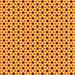
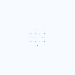
6. Kekule-O (topological) distorted graphene with $(\sqrt{3}\times\sqrt{3})R30^\circ$ superlattice.
|
|
331
|
+
- `Moire lattice`: bilayer
|
|
332
|
+
- `Simple`
|
|
333
|
+
- `eta` $\eta$ : 0.5
|
|
334
|
+
- `L = 7`
|
|
335
|
+
- `Pixels = 256`
|
|
336
|
+
- `Theta = 0`
|
|
337
|
+
- Lattice 1:
|
|
338
|
+
- Parameters:
|
|
339
|
+
- `Hexagonal`, `a = 0.3`
|
|
340
|
+
- Sublattices:
|
|
341
|
+
- `Hollow`, `alpha1 = 1`, `beta1 = 1`
|
|
342
|
+
- Strain:
|
|
343
|
+
- `e11` = `e12` = `e22` = `0`
|
|
344
|
+
- Lattice 2:
|
|
345
|
+
- Parameters:
|
|
346
|
+
- `Hexagonal`, `b = 0.3*sqrt(3)`, `Twist angle = 30`
|
|
347
|
+
- Sublattices:
|
|
348
|
+
- `Hollow`, `alpha2 = 1`, `beta2 = 1`
|
|
349
|
+
- Strain:
|
|
350
|
+
- `d11` = `d12` = `d22` = `0`
|
|
351
|
+
|
|
352
|
+
|
|
353
|
+
|
|
354
|
+
|
|
@@ -0,0 +1,337 @@
|
|
|
1
|
+
# PyAtoms
|
|
2
|
+
|
|
3
|
+
|
|
4
|
+
Simulates scanning probe microscopy (SPM) images. Please read our preprint describing PyAtoms: <a href="https://arxiv.org/abs/2412.18332" target="__blank" rel="noopener noreferrer"> https://arxiv.org/abs/2412.18332. </a>
|
|
5
|
+
|
|
6
|
+
(Formerly named: SPM Simulator, Atom Simulator)
|
|
7
|
+
|
|
8
|
+
|
|
9
|
+

|
|
10
|
+
|
|
11
|
+
|
|
12
|
+
### Dependencies:
|
|
13
|
+
- Python 3.0 or newer
|
|
14
|
+
- NumPy
|
|
15
|
+
- Matplotlib
|
|
16
|
+
- SciPy
|
|
17
|
+
- QtPy
|
|
18
|
+
- PyQt5 or PyQt6
|
|
19
|
+
|
|
20
|
+
PyAtoms is compatible with both PyQt5 and PyQt6 through QtPy. PyQt6 is installed by default when PyAtoms is installed using pip.
|
|
21
|
+
|
|
22
|
+
## Installation instructions - macOS and WIndows
|
|
23
|
+
|
|
24
|
+
### Install with pip
|
|
25
|
+
|
|
26
|
+
PyAtoms can be installed using pip:
|
|
27
|
+
|
|
28
|
+
```bash
|
|
29
|
+
pip install pyatoms-spm
|
|
30
|
+
```
|
|
31
|
+
|
|
32
|
+
After installation, launch PyAtoms by typing:
|
|
33
|
+
|
|
34
|
+
```bash
|
|
35
|
+
pyatoms
|
|
36
|
+
```
|
|
37
|
+
|
|
38
|
+
### Run from source
|
|
39
|
+
|
|
40
|
+
PyAtoms can also be run directly from the source code.
|
|
41
|
+
|
|
42
|
+
1. Click the green **Code** button at the top of this GitHub page and select **Download ZIP**.
|
|
43
|
+
|
|
44
|
+
2. Extract the downloaded ZIP file.
|
|
45
|
+
|
|
46
|
+
3. Open a terminal or command line:
|
|
47
|
+
- **Windows:** open Command Prompt, PowerShell, or the Anaconda Prompt.
|
|
48
|
+
- **macOS:** open the Terminal application.
|
|
49
|
+
|
|
50
|
+
4. In the terminal, navigate to the extracted PyAtoms folder.
|
|
51
|
+
|
|
52
|
+
If the ZIP was extracted into your Downloads folder, you can usually use:
|
|
53
|
+
|
|
54
|
+
**Windows Command Prompt:**
|
|
55
|
+
|
|
56
|
+
```bash
|
|
57
|
+
cd %USERPROFILE%\Downloads\PyAtoms-main
|
|
58
|
+
```
|
|
59
|
+
|
|
60
|
+
**Wndows PowerShell:**
|
|
61
|
+
|
|
62
|
+
```powershell
|
|
63
|
+
cd "$HOME\Downloads\PyAtoms-main"
|
|
64
|
+
```
|
|
65
|
+
|
|
66
|
+
**macOS:**
|
|
67
|
+
|
|
68
|
+
```bash
|
|
69
|
+
cd ~/Downloads/PyAtoms-main
|
|
70
|
+
```
|
|
71
|
+
|
|
72
|
+
If you extracted the folder somewhere else, replace the path above with the location of your extracted PyAtoms folder.
|
|
73
|
+
|
|
74
|
+
5. Install the required Python packages.
|
|
75
|
+
|
|
76
|
+
For PyQt6:
|
|
77
|
+
|
|
78
|
+
```bash
|
|
79
|
+
python -m pip install numpy scipy matplotlib QtPy PyQt6
|
|
80
|
+
```
|
|
81
|
+
|
|
82
|
+
Or, if you use PyQt5:
|
|
83
|
+
|
|
84
|
+
```bash
|
|
85
|
+
python -m pip install numpy scipy matplotlib QtPy PyQt5
|
|
86
|
+
```
|
|
87
|
+
|
|
88
|
+
6. From inside the extracted PyAtoms folder, start PyAtoms with:
|
|
89
|
+
|
|
90
|
+
```bash
|
|
91
|
+
python -m pyatoms.PyAtoms_GUI
|
|
92
|
+
```
|
|
93
|
+
|
|
94
|
+
PyAtoms is compatile with both PyQt5 and PyQt6 through QtPy.
|
|
95
|
+
|
|
96
|
+
## Known issues
|
|
97
|
+
|
|
98
|
+
02-Sep-2026: Pyatoms is compatile with both PyQt5 and PyQt6 through QtPy. PyQt6 is installed by default when installing PyAtoms through pip.
|
|
99
|
+
|
|
100
|
+
06-Nov-2025: PyAtoms is currently **not** compatible with PyQt 6. Still compatible with latest PyQt5 (5.15.11)
|
|
101
|
+
|
|
102
|
+
28-Oct-2024: No known issues. Works correctly with latest version of Matplotlib (3.9.2)
|
|
103
|
+
|
|
104
|
+
### For windows users:
|
|
105
|
+
- Make sure python is installed and that its path is set in your environment
|
|
106
|
+
- To check if it is, open the command line and type
|
|
107
|
+
```
|
|
108
|
+
python -V
|
|
109
|
+
```
|
|
110
|
+
- Alternatively, if you installed python, NumPy, SciPy, etc. through Anaconda for Windows, you can run the above code through the Anaconda prompt.
|
|
111
|
+
|
|
112
|
+
For any other issues or crash reports, suggestions, contact gutierrez@physics.ucla.edu
|
|
113
|
+
|
|
114
|
+
##
|
|
115
|
+
## How to use
|
|
116
|
+
|
|
117
|
+

|
|
118
|
+
|
|
119
|
+
|
|
120
|
+
Note that all fields accept typical mathematical operations in python and NumPy such as `+` `-` `*` `/` `sqrt` `log` and all valid NumPy functions `func` can be called via `np.func()`.
|
|
121
|
+
|
|
122
|
+
1. **Number of lattices** (moiré, CDW, superlattice) and **Moiré model** (Simple, Log)
|
|
123
|
+
- Choose to simulate a 1, 2 or 3 layer lattice
|
|
124
|
+
- Lattice 1 parameters change the single/first layer.
|
|
125
|
+
- Lattice 2 only works if bilayer/trilayer are selected. These change the second lattice.
|
|
126
|
+
- Lattice 3 only works if trilayer is selected. These change the third lattice.
|
|
127
|
+
- Choose the model to simulate the moiré/CDW/superlattice
|
|
128
|
+
- `Simple`: This minimal toy model approximates the moiré image, $T_M$, as the weighted sum between the sum of the individual lattices, $\sum_l Z_l$, and the product of the lattices, $\prod_l Z_l$ and is given by $T_M \propto (1-\eta)\sum_l Z_l + \eta\prod_L Z_l$. This toy model provides a good match to experimental STM images and offers a wide image contrast. However, the Fourier transforms -- by design -- contains only the first order atomic Bragg and moiré lattice peaks. The image is normalized such that $0\leq T_M \leq 1$.
|
|
129
|
+
- `eta`, $\eta$ : A phenomenological parameter we use to weigh the relative strength of the sum of lattices, $\sum_l Z_l$, to the product of lattices, $\prod_L Z_l$. $\eta$ is a real number between 0 and 1: The moiré/superlattice image for $\eta=0$ purely the sum and $\eta=1$ is purely the product.
|
|
130
|
+
- `Log`: This model, described by Joucken *et al* (<a href="https://doi.org/10.1016/j.carbon.2014.11.030" target="_blank" rel="noopener noreferrer"> *Carbon* **83**, 48 (2015). </a>) is rooted in the constant-current tunneling process and takes into account the distance of the multilayers to the STM tip. The moiré/superlattice image, $T_M^L$, is approximated as $T_M^L \propto \ln|Z_1 + Z_2 e^{-\xi}|$ (bilayer) or $T_M^L \propto \ln|Z_1 + Z_2 e^{-\xi} + Z_3 e^{-2\xi}|$ (trilayer). This model provides a good match to both experimental STM images and their Fourier transforms, at the cost of limited image contrast.
|
|
131
|
+
- `xi`, $\xi$ : The ratio of the inter-layer distance, $d$, and out-of-plane wavefunction decay length, $\lambda$: $\xi = d/\lambda$. $\xi$ is a real number between 0 and 10: For $\xi=0$, the intensity of the lattices is maximized; for $\xi$ = 10, only the top lattice, $Z_1$, is imaged.
|
|
132
|
+
|
|
133
|
+
2. Image parameters
|
|
134
|
+
- `Real resolution`: Current spatial resolution, defined as L/pix, in units of nm/pix.
|
|
135
|
+
- `K-space resolution`: Current spatial resolution in reciprocal space, defined as 2π/L, in units of nm⁻¹/pix.
|
|
136
|
+
- `Pixels`: number of pixels. Must be an integer or a mathematical expression of integers.
|
|
137
|
+
- `Image length, L`: length of the image window in nanometers. Must be a real number or a mathematical expression of real numbers.
|
|
138
|
+
- `Scan angle, θ`: Rotation (counter-clockwise) of the atomic lattice. Must be a real number or a mathematical expression of real numbers.
|
|
139
|
+
- `Image offset`: Location of center of image. Must be a pair of real numbers, or a mathematical expression of real numbers, separated by a comma, e.g. -1.2,4.5.
|
|
140
|
+
|
|
141
|
+
3. Colormap
|
|
142
|
+
- `Real space image`: colormap of the real space simulated atomic lattice.
|
|
143
|
+
- `FFT`: colormap of the 2D fast Fourier transform.
|
|
144
|
+
|
|
145
|
+
4. Low pass filtering
|
|
146
|
+
- `Gaussian width, σ`: radius of a Gaussian mask in real space in units of pixels. The half-width at half-max of the gaussian is shown as a white circle in the bottom left corner of the image.
|
|
147
|
+
- The radius of the gaussian mask in nanometers is shown in the text box.
|
|
148
|
+
|
|
149
|
+
5. Save files
|
|
150
|
+
- Click to save the files to a specific directory.
|
|
151
|
+
- Clicking will open the file explorer.
|
|
152
|
+
- Navigate to the directory you want to save the files in
|
|
153
|
+
- Input a `filename` to save as
|
|
154
|
+
- It will save a folder called `filename` with 4 files:
|
|
155
|
+
- .png images of the real space and FFT, .txt file of the real space image, .txt file of the parameter values
|
|
156
|
+
- `filename.png`, `filename_FFT.png`, `filename.txt`, `filename_params.txt`
|
|
157
|
+
- Example of folder with saved files:
|
|
158
|
+
|
|
159
|
+
<img width="700" alt="Screen Shot 2022-08-04 at 1 30 29 PM" src="https://user-images.githubusercontent.com/62832051/182946811-ba2a1e4d-04d7-4658-b013-38dac1c8ef42.png">
|
|
160
|
+
- Example of params .txt file:
|
|
161
|
+
|
|
162
|
+
<img width="446" alt="Screen Shot 2022-08-03 at 3 40 46 PM" src="https://user-images.githubusercontent.com/62832051/182724722-b820f3b3-a2e2-413c-8c9d-cb03da7b78ce.png">
|
|
163
|
+
|
|
164
|
+
|
|
165
|
+
6. SPM image time estimator
|
|
166
|
+
- `Tip velocity`: Velocity of the tip, $v_t$ across 1 line in nanometers/second. The total image time is calculated by considering the total pixels, scanning left/right and in a single slow-scan direction (upwards, for example). This time is estimated via $T_{im} = (2 * N_{pix} * L) / v_t$, where $N_{pix}$ is the number of pixels in the image, $L$ is the length of the image in nanometers, and the factor 2 takes into account the left/right fast-scan direction.
|
|
167
|
+
|
|
168
|
+
7. Spectroscopy map Time estimator
|
|
169
|
+
- `Time per spectra`: Total time in seconds (including overhead) to record a single spectrum, $T_{spec}$ i.e. one dI/dV(V) sweep. We assume that spectra are recorded in one direction along both the fast- and slow-scan direction. The time is estimated via $T_{map} = N_{pix}^2 * T_{spec} + (2 * N_{pix} * L) / v_t$.
|
|
170
|
+
|
|
171
|
+
8. Lattices
|
|
172
|
+
- Parameters tab
|
|
173
|
+
- `symmetry`: Choose to simulate either a triangular/hexagonal or square lattice.
|
|
174
|
+
- `Lattice constant`: periodicity/spacing between atoms in nanometers.
|
|
175
|
+
- `Twist angle`: twists the second lattice with respect to the first lattice (in Lattice 2 params) // twists the third lattice with respect to the second lattice (in Lattice 3 params)
|
|
176
|
+
|
|
177
|
+
- Sublattices tab -- only affects hexagonal (triangular/honeycomb) lattices
|
|
178
|
+
- Lattice site at the image `origin`: choose whether the `origin` should be a hollow site, an A-site atom or a B-site atom
|
|
179
|
+
- To test this, set `L = 1` and click the different options for the origin
|
|
180
|
+
<img width="400" alt="Screen Shot 2022-10-03 at 4 26 18 PM" src="https://user-images.githubusercontent.com/62832051/193703355-855b46de-f020-428f-af81-0ae4fee0bf57.png">
|
|
181
|
+
|
|
182
|
+
|
|
183
|
+
- Weight of sublattices:
|
|
184
|
+
- `alpha1`, $\alpha_1$ : weight of A sublattice
|
|
185
|
+
- `beta1`, $\beta_1$: weight of B sublattice
|
|
186
|
+
- For a triangular lattice: `alpha = 1`, `beta = 0`
|
|
187
|
+
|
|
188
|
+

|
|
189
|
+
|
|
190
|
+
- For a honeycomb lattice: `alpha = 1`, `beta = 1`
|
|
191
|
+
|
|
192
|
+

|
|
193
|
+
|
|
194
|
+
- Strain tab
|
|
195
|
+
- Apply the 2D strain tensor, $e_{xy}$, where the $x$-axis is defined as the *local* direction of that lattice, i.e. the strain tensor rotates with the local axes set by `theta` or `twist angle`. See https://doi.org/10.1103/PhysRevB.80.045401.
|
|
196
|
+
|
|
197
|
+
|
|
198
|
+
##
|
|
199
|
+
## Examples
|
|
200
|
+
1. Twisted bilayer graphene with $1.1^\circ$ twist angle.
|
|
201
|
+
- `Moire lattice`: bilayer
|
|
202
|
+
- `Simple`
|
|
203
|
+
- `eta` $\eta$ : 0.5
|
|
204
|
+
- `L = 35`
|
|
205
|
+
- `Pixels = 1024`
|
|
206
|
+
- Lattice 1:
|
|
207
|
+
- Parameters:
|
|
208
|
+
- `Hexagonal`, `a = 0.3`
|
|
209
|
+
- Sublattices:
|
|
210
|
+
- `A-site`, `alpha1 = 1`, `beta1 = 1`
|
|
211
|
+
- Strain:
|
|
212
|
+
- `e11` = `e12` = `e22` = `0`
|
|
213
|
+
- Lattice 2:
|
|
214
|
+
- Parameters:
|
|
215
|
+
- `Hexagonal`, `b = 0.3`, `Twist angle = 1.1`
|
|
216
|
+
- Sublattices:
|
|
217
|
+
- `A-site`, `alpha2 = 1`, `beta2 = 1`
|
|
218
|
+
- Strain:
|
|
219
|
+
- `d11` = `d12` = `d22` = `0`
|
|
220
|
+
|
|
221
|
+
<img width="260" alt="Screen Shot 2022-08-05 at 1 41 35 PM" src="https://user-images.githubusercontent.com/62832051/183159495-dc4b4c38-5e67-4cbc-bbe9-55ff9b696ec6.png">
|
|
222
|
+
|
|
223
|
+
<img width="280" alt="Screen Shot 2022-08-03 at 3 43 14 PM" src="https://user-images.githubusercontent.com/62832051/182725026-1a462df7-9372-4b7e-bd02-6041134966b7.png">
|
|
224
|
+
|
|
225
|
+
|
|
226
|
+
|
|
227
|
+
2. 1T-TaS2 with $(\sqrt{13}\times\sqrt{13})R13.9^\circ$ charge density wave superlattice.
|
|
228
|
+
- `Moire lattice`: bilayer
|
|
229
|
+
- `Simple`
|
|
230
|
+
- `eta` $\eta$ : 0.5
|
|
231
|
+
- `L = 7`
|
|
232
|
+
- `Pixels = 256`
|
|
233
|
+
- `Theta = 0 `
|
|
234
|
+
- Lattice 1:
|
|
235
|
+
- Parameters:
|
|
236
|
+
- `Hexagonal`, `a = 0.3`
|
|
237
|
+
- Sublattices:
|
|
238
|
+
- `A-site`, `alpha1 = 1`, `beta1 = 0`
|
|
239
|
+
- Strain:
|
|
240
|
+
- `e11` = `e12` = `e22` = `0`
|
|
241
|
+
- Lattice 2:
|
|
242
|
+
- Parameters:
|
|
243
|
+
- `Hexagonal`, `b = 0.3*np.sqrt(13)`, `Twist angle = 13.9`
|
|
244
|
+
- Sublattices:
|
|
245
|
+
- `A-site`, `alpha2 = 1`, `beta2 = 0`
|
|
246
|
+
- Strain:
|
|
247
|
+
- `d11` = `d12` = `d22` = `0`
|
|
248
|
+
|
|
249
|
+

|
|
250
|
+

|
|
251
|
+
|
|
252
|
+
|
|
253
|
+
3. 2H-NbSe2 with $(3\times 3)R0^\circ$ charge density wave superlattice.
|
|
254
|
+
- `Moire lattice`: bilayer
|
|
255
|
+
- `Simple`
|
|
256
|
+
- `eta` $\eta$ : 0.5
|
|
257
|
+
- `L = 7`
|
|
258
|
+
- `Pixels = 256`
|
|
259
|
+
- `Theta = 0`
|
|
260
|
+
- Lattice 1:
|
|
261
|
+
- Parameters:
|
|
262
|
+
- `Hexagonal`, `a = 0.3`
|
|
263
|
+
- Sublattices:
|
|
264
|
+
- `A-site`, `alpha1 = 1`, `beta1 = 0`
|
|
265
|
+
- Strain:
|
|
266
|
+
- `e11` = `e12` = `e22` = `0`
|
|
267
|
+
- Lattice 2:
|
|
268
|
+
- Parameters:
|
|
269
|
+
- `Hexagonal`, `b = 0.3*3`, `Twist angle = 0`
|
|
270
|
+
- Sublattices:
|
|
271
|
+
- `A-site`, `alpha2 = 1`, `beta2 = 0`
|
|
272
|
+
- Strain:
|
|
273
|
+
- `d11` = `d12` = `d22` = `0`
|
|
274
|
+
|
|
275
|
+

|
|
276
|
+

|
|
277
|
+
|
|
278
|
+
Here is an example where PyAtoms can simulate real data.
|
|
279
|
+
|
|
280
|
+
Top: Experimental measurement of NbSe2 showing a CDW phase gradient from bond- to site-centered from Sanna *et al* <a href="https://rdcu.be/dSFwq" target="_blank" rel="noopener noreferrer"> *npj Quantum Materials* **7**, 6 (2022). </a>
|
|
281
|
+
|
|
282
|
+
Bottom: PyAtoms simulation of this phase gradient by adding a small discommensuration term, δ, so that the CDW superlattice is given by (3 + δ)x(3 + δ)R0°.
|
|
283
|
+
|
|
284
|
+
<img width="489" alt="image" src="https://github.com/user-attachments/assets/c61bf104-e246-4d5a-8032-232ca81e0c39" />
|
|
285
|
+
|
|
286
|
+
|
|
287
|
+
5. Kekule-O (trivial) distorted graphene with $(\sqrt{3}\times\sqrt{3})R30^\circ$ superlattice.
|
|
288
|
+
- `Moire lattice`: bilayer
|
|
289
|
+
- `Simple`
|
|
290
|
+
- `eta` $\eta$ : 0.5
|
|
291
|
+
- `L = 7`
|
|
292
|
+
- `Pixels = 256`
|
|
293
|
+
- `Theta = 0`
|
|
294
|
+
- Lattice 1:
|
|
295
|
+
- Parameters:
|
|
296
|
+
- `Hexagonal`, `a = 0.3`
|
|
297
|
+
- Sublattices:
|
|
298
|
+
- `Hollow`, `alpha1 = 1`, `beta1 = 1`
|
|
299
|
+
- Strain:
|
|
300
|
+
- `e11` = `e12` = `e22` = `0`
|
|
301
|
+
- Lattice 2:
|
|
302
|
+
- Parameters:
|
|
303
|
+
- `Hexagonal`, `b = 0.3*sqrt(3)`, `Twist angle = 30`
|
|
304
|
+
- Sublattices:
|
|
305
|
+
- `Hollow`, `alpha2 = 1`, `beta2 = 0`
|
|
306
|
+
- Strain:
|
|
307
|
+
- `d11` = `d12` = `d22` = `0`
|
|
308
|
+
|
|
309
|
+

|
|
310
|
+

|
|
311
|
+
|
|
312
|
+
|
|
313
|
+
6. Kekule-O (topological) distorted graphene with $(\sqrt{3}\times\sqrt{3})R30^\circ$ superlattice.
|
|
314
|
+
- `Moire lattice`: bilayer
|
|
315
|
+
- `Simple`
|
|
316
|
+
- `eta` $\eta$ : 0.5
|
|
317
|
+
- `L = 7`
|
|
318
|
+
- `Pixels = 256`
|
|
319
|
+
- `Theta = 0`
|
|
320
|
+
- Lattice 1:
|
|
321
|
+
- Parameters:
|
|
322
|
+
- `Hexagonal`, `a = 0.3`
|
|
323
|
+
- Sublattices:
|
|
324
|
+
- `Hollow`, `alpha1 = 1`, `beta1 = 1`
|
|
325
|
+
- Strain:
|
|
326
|
+
- `e11` = `e12` = `e22` = `0`
|
|
327
|
+
- Lattice 2:
|
|
328
|
+
- Parameters:
|
|
329
|
+
- `Hexagonal`, `b = 0.3*sqrt(3)`, `Twist angle = 30`
|
|
330
|
+
- Sublattices:
|
|
331
|
+
- `Hollow`, `alpha2 = 1`, `beta2 = 1`
|
|
332
|
+
- Strain:
|
|
333
|
+
- `d11` = `d12` = `d22` = `0`
|
|
334
|
+
|
|
335
|
+

|
|
336
|
+

|
|
337
|
+
|