popgrid 0.4.0__tar.gz
This diff represents the content of publicly available package versions that have been released to one of the supported registries. The information contained in this diff is provided for informational purposes only and reflects changes between package versions as they appear in their respective public registries.
- popgrid-0.4.0/LICENSE +21 -0
- popgrid-0.4.0/PKG-INFO +184 -0
- popgrid-0.4.0/README.md +149 -0
- popgrid-0.4.0/popgrid/__init__.py +40 -0
- popgrid-0.4.0/popgrid/cartogram.py +747 -0
- popgrid-0.4.0/popgrid/core.py +1127 -0
- popgrid-0.4.0/popgrid/data.py +432 -0
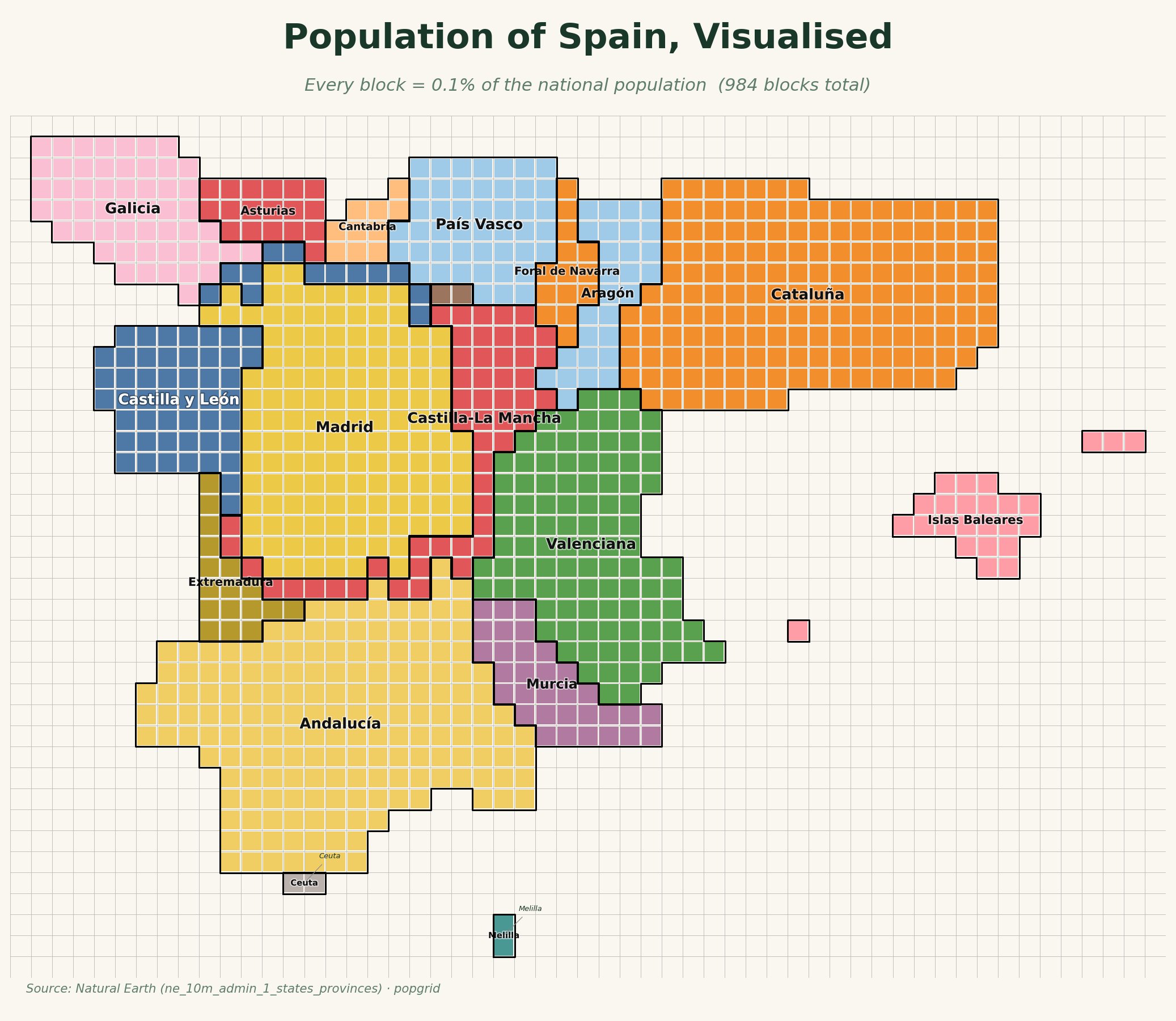
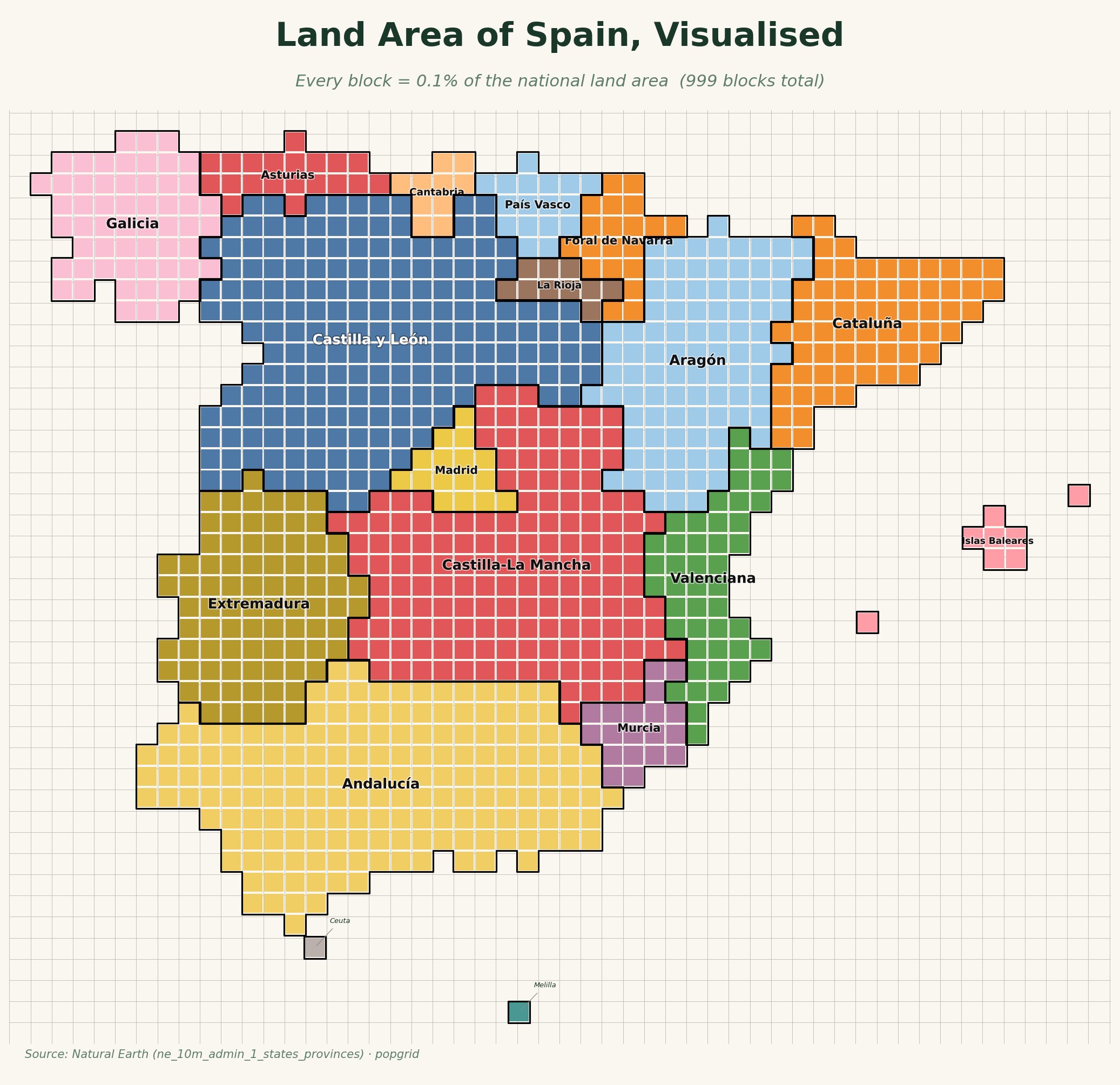
- popgrid-0.4.0/popgrid/exceptions.py +19 -0
- popgrid-0.4.0/popgrid/geometry.py +223 -0
- popgrid-0.4.0/popgrid/grid.py +231 -0
- popgrid-0.4.0/popgrid/render.py +954 -0
- popgrid-0.4.0/popgrid/resources/population.csv +797 -0
- popgrid-0.4.0/popgrid.egg-info/PKG-INFO +184 -0
- popgrid-0.4.0/popgrid.egg-info/SOURCES.txt +21 -0
- popgrid-0.4.0/popgrid.egg-info/dependency_links.txt +1 -0
- popgrid-0.4.0/popgrid.egg-info/requires.txt +13 -0
- popgrid-0.4.0/popgrid.egg-info/top_level.txt +1 -0
- popgrid-0.4.0/pyproject.toml +56 -0
- popgrid-0.4.0/setup.cfg +4 -0
- popgrid-0.4.0/tests/test_core.py +363 -0
- popgrid-0.4.0/tests/test_data.py +122 -0
- popgrid-0.4.0/tests/test_geometry.py +141 -0
- popgrid-0.4.0/tests/test_grid.py +179 -0
popgrid-0.4.0/LICENSE
ADDED
|
@@ -0,0 +1,21 @@
|
|
|
1
|
+
MIT License
|
|
2
|
+
|
|
3
|
+
Copyright (c) 2026 Josep Ferrer
|
|
4
|
+
|
|
5
|
+
Permission is hereby granted, free of charge, to any person obtaining a copy
|
|
6
|
+
of this software and associated documentation files (the "Software"), to deal
|
|
7
|
+
in the Software without restriction, including without limitation the rights
|
|
8
|
+
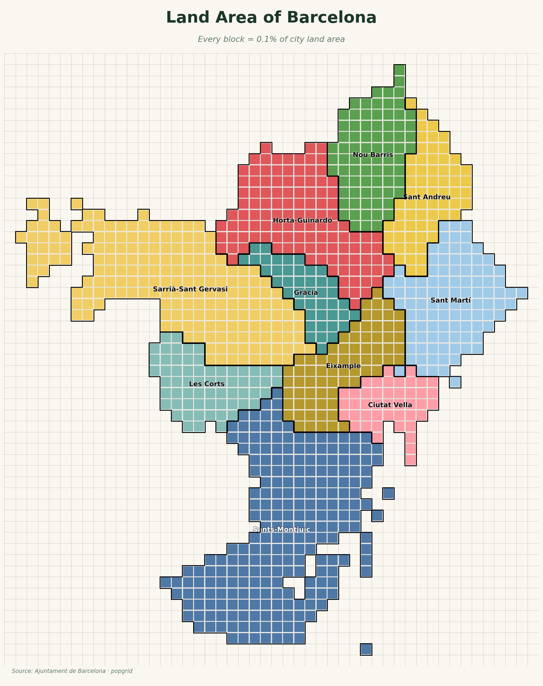
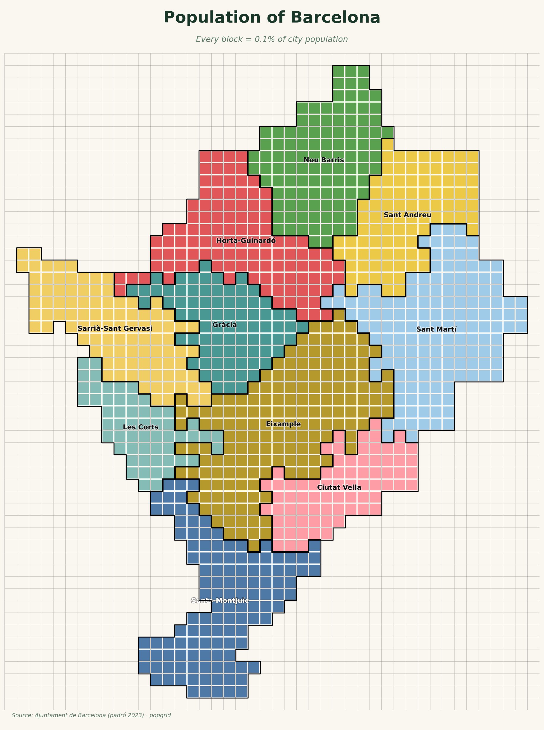
to use, copy, modify, merge, publish, distribute, sublicense, and/or sell
|
|
9
|
+
copies of the Software, and to permit persons to whom the Software is
|
|
10
|
+
furnished to do so, subject to the following conditions:
|
|
11
|
+
|
|
12
|
+
The above copyright notice and this permission notice shall be included in all
|
|
13
|
+
copies or substantial portions of the Software.
|
|
14
|
+
|
|
15
|
+
THE SOFTWARE IS PROVIDED "AS IS", WITHOUT WARRANTY OF ANY KIND, EXPRESS OR
|
|
16
|
+
IMPLIED, INCLUDING BUT NOT LIMITED TO THE WARRANTIES OF MERCHANTABILITY,
|
|
17
|
+
FITNESS FOR A PARTICULAR PURPOSE AND NONINFRINGEMENT. IN NO EVENT SHALL THE
|
|
18
|
+
AUTHORS OR COPYRIGHT HOLDERS BE LIABLE FOR ANY CLAIM, DAMAGES OR OTHER
|
|
19
|
+
LIABILITY, WHETHER IN AN ACTION OF CONTRACT, TORT OR OTHERWISE, ARISING FROM,
|
|
20
|
+
OUT OF OR IN CONNECTION WITH THE SOFTWARE OR THE USE OR OTHER DEALINGS IN THE
|
|
21
|
+
SOFTWARE.
|
popgrid-0.4.0/PKG-INFO
ADDED
|
@@ -0,0 +1,184 @@
|
|
|
1
|
+
Metadata-Version: 2.4
|
|
2
|
+
Name: popgrid
|
|
3
|
+
Version: 0.4.0
|
|
4
|
+
Summary: Tiled grid maps for Python — land area and population cartograms
|
|
5
|
+
Author-email: Josep Ferrer <rfeers@gmail.com>
|
|
6
|
+
License: MIT
|
|
7
|
+
Project-URL: Homepage, https://databites.tech
|
|
8
|
+
Project-URL: Repository, https://github.com/databites-tech/popgrid
|
|
9
|
+
Project-URL: Issues, https://github.com/databites-tech/popgrid/issues
|
|
10
|
+
Keywords: dataviz,maps,population,cartography,geopandas,visualization
|
|
11
|
+
Classifier: Programming Language :: Python :: 3
|
|
12
|
+
Classifier: Programming Language :: Python :: 3.10
|
|
13
|
+
Classifier: Programming Language :: Python :: 3.11
|
|
14
|
+
Classifier: Programming Language :: Python :: 3.12
|
|
15
|
+
Classifier: License :: OSI Approved :: MIT License
|
|
16
|
+
Classifier: Intended Audience :: Science/Research
|
|
17
|
+
Classifier: Topic :: Scientific/Engineering :: Visualization
|
|
18
|
+
Classifier: Topic :: Scientific/Engineering :: GIS
|
|
19
|
+
Requires-Python: >=3.10
|
|
20
|
+
Description-Content-Type: text/markdown
|
|
21
|
+
License-File: LICENSE
|
|
22
|
+
Requires-Dist: geopandas>=0.14
|
|
23
|
+
Requires-Dist: shapely>=2.0
|
|
24
|
+
Requires-Dist: matplotlib>=3.7
|
|
25
|
+
Requires-Dist: numpy>=1.24
|
|
26
|
+
Requires-Dist: requests>=2.28
|
|
27
|
+
Requires-Dist: pycountry>=22.0
|
|
28
|
+
Requires-Dist: pyproj>=3.5
|
|
29
|
+
Provides-Extra: dev
|
|
30
|
+
Requires-Dist: pytest>=7; extra == "dev"
|
|
31
|
+
Requires-Dist: ruff; extra == "dev"
|
|
32
|
+
Requires-Dist: black; extra == "dev"
|
|
33
|
+
Requires-Dist: ipykernel; extra == "dev"
|
|
34
|
+
Dynamic: license-file
|
|
35
|
+
|
|
36
|
+
# popgrid
|
|
37
|
+
|
|
38
|
+
**Tiled grid maps for Python, land area and population, clearly explained.**
|
|
39
|
+
|
|
40
|
+
[](https://pypi.org/project/popgrid/)
|
|
41
|
+
[](https://pypi.org/project/popgrid/)
|
|
42
|
+
[](LICENSE)
|
|
43
|
+
|
|
44
|
+
popgrid turns a country (or any set of regions) into a block cartogram where **every block is an equal share of the whole**: 0.1% of the national land area, or 0.1% of the population. Same regions, same colours, two ways of seeing them. Where land and people diverge is the whole point.
|
|
45
|
+
|
|
46
|
+
<p align="center">
|
|
47
|
+
<img src="https://raw.githubusercontent.com/databites-tech/popgrid/main/docs/img/spain_compare.png" width="100%" alt="Land area vs population of Spain, side by side">
|
|
48
|
+
</p>
|
|
49
|
+
|
|
50
|
+
Madrid is a sliver of land and a giant of population. The empty interior shrinks; the coasts and the capital swell. A block on the left is the same size as a block on the right, so the comparison is literally true.
|
|
51
|
+
|
|
52
|
+
---
|
|
53
|
+
|
|
54
|
+
## Install
|
|
55
|
+
|
|
56
|
+
```bash
|
|
57
|
+
pip install popgrid
|
|
58
|
+
```
|
|
59
|
+
|
|
60
|
+
Requires Python 3.10+. Country boundaries are downloaded once from Natural Earth and cached locally; population data for the bundled countries ships with the package.
|
|
61
|
+
|
|
62
|
+
---
|
|
63
|
+
|
|
64
|
+
## Quickstart
|
|
65
|
+
|
|
66
|
+
```python
|
|
67
|
+
from popgrid import PopGrid, AreaGrid
|
|
68
|
+
|
|
69
|
+
# Population: every block = 0.1% of the national population
|
|
70
|
+
PopGrid("ESP").plot().savefig("spain_population.png", dpi=170, bbox_inches="tight")
|
|
71
|
+
|
|
72
|
+
# Land area: every block = 0.1% of the national land area
|
|
73
|
+
AreaGrid("ESP").plot().savefig("spain_area.png", dpi=170, bbox_inches="tight")
|
|
74
|
+
```
|
|
75
|
+
|
|
76
|
+
| Population | Land area |
|
|
77
|
+
|---|---|
|
|
78
|
+
|  |  |
|
|
79
|
+
|
|
80
|
+
`.plot()` builds the grid on first call and returns a Matplotlib figure, so you can save, show, or restyle it however you like.
|
|
81
|
+
|
|
82
|
+
---
|
|
83
|
+
|
|
84
|
+
## Your own data
|
|
85
|
+
|
|
86
|
+
Both classes accept any GeoDataFrame through `from_geodataframe`, so popgrid is not limited to the bundled countries. Point it at a shapefile, a GeoJSON, or a PostGIS query.
|
|
87
|
+
|
|
88
|
+
- `AreaGrid.from_geodataframe(gdf, region_col=...)` sizes each region by its land area.
|
|
89
|
+
- `PopGrid.from_geodataframe(gdf, region_col=..., weight_col=...)` sizes each region by a numeric column you supply, such as population.
|
|
90
|
+
|
|
91
|
+
```python
|
|
92
|
+
import geopandas as gpd
|
|
93
|
+
from popgrid import AreaGrid, PopGrid
|
|
94
|
+
|
|
95
|
+
gdf = gpd.read_file("examples/data/barcelona_districts.geojson")
|
|
96
|
+
|
|
97
|
+
# Sized by district land area
|
|
98
|
+
AreaGrid.from_geodataframe(gdf, region_col="district").plot(
|
|
99
|
+
title="Land Area of Barcelona",
|
|
100
|
+
subtitle="Every block = 0.1% of city land area",
|
|
101
|
+
)
|
|
102
|
+
|
|
103
|
+
# Sized by your own population column
|
|
104
|
+
PopGrid.from_geodataframe(gdf, region_col="district", weight_col="population").plot(
|
|
105
|
+
title="Population of Barcelona",
|
|
106
|
+
subtitle="Every block = 0.1% of city population",
|
|
107
|
+
)
|
|
108
|
+
```
|
|
109
|
+
|
|
110
|
+
Barcelona's 10 districts, built entirely from a custom GeoDataFrame. Eixample, the densest district, balloons under population; Les Corts and the green hills of Sarrià shrink.
|
|
111
|
+
|
|
112
|
+
| Land area | Population |
|
|
113
|
+
|---|---|
|
|
114
|
+
|  |  |
|
|
115
|
+
|
|
116
|
+
A full runnable version is in [`examples/barcelona.py`](examples/barcelona.py), using the district boundaries in [`examples/data/barcelona_districts.geojson`](examples/data/barcelona_districts.geojson).
|
|
117
|
+
|
|
118
|
+
---
|
|
119
|
+
|
|
120
|
+
## Command line
|
|
121
|
+
|
|
122
|
+
`generate.py` (at the repo root) renders one or many countries from the terminal.
|
|
123
|
+
|
|
124
|
+
```bash
|
|
125
|
+
# Population map of Spain
|
|
126
|
+
python generate.py ESP --mode pop
|
|
127
|
+
|
|
128
|
+
# Land-area map
|
|
129
|
+
python generate.py ESP --mode area
|
|
130
|
+
|
|
131
|
+
# Side-by-side comparison (land area vs population, equal block size)
|
|
132
|
+
python generate.py ESP --mode compare
|
|
133
|
+
|
|
134
|
+
# Several countries at once, into a folder
|
|
135
|
+
python generate.py ESP DEU FRA --mode compare --out compare/
|
|
136
|
+
|
|
137
|
+
# Everything bundled
|
|
138
|
+
python generate.py ALL --mode pop
|
|
139
|
+
```
|
|
140
|
+
|
|
141
|
+
Useful flags: `--n` (target block count, default 1000), `--mainland` (drop detached territories), `--no-panels` (keep nearby islands inline, drop distant panels), `--palette`, `--dissolve`, `--no-labels`, `--bg`, `--background grid|solid|none`, `--title`, `--subtitle`, `--source`, `--dpi`, `--out`. Run `python generate.py --help` for the full list.
|
|
142
|
+
|
|
143
|
+
---
|
|
144
|
+
|
|
145
|
+
## Bundled countries
|
|
146
|
+
|
|
147
|
+
24 countries ship with population data and recommended regional segmentation:
|
|
148
|
+
|
|
149
|
+
`ARG` `AUS` `BEL` `BRA` `CAN` `CHE` `CHN` `DEU` `ESP` `FRA` `GBR` `ITA` `JPN` `KOR` `MEX` `NLD` `NOR` `PHL` `POL` `PRT` `SWE` `TUR` `USA` `ZAF`
|
|
150
|
+
|
|
151
|
+
For any other country, or for sub-national data such as cities, use `from_geodataframe` with your own polygons.
|
|
152
|
+
|
|
153
|
+
---
|
|
154
|
+
|
|
155
|
+
## How it works
|
|
156
|
+
|
|
157
|
+
1. Load admin-1 regions, project to an equal-area CRS, and choose a cell size so the country tiles into roughly `n` blocks (default 1000, so one block ≈ 0.1%).
|
|
158
|
+
2. Allocate an integer block quota per region using the Hamilton (largest-remainder) method, weighted by area or population.
|
|
159
|
+
3. For population maps, deform each landmass with a contiguous-area cartogram so a region's area tracks its population, then rasterise the deformed shapes onto the grid. Dense regions bulge, sparse regions pinch, relative position and silhouette are preserved.
|
|
160
|
+
4. Fit each region to its exact quota and assign stable colours from the geographic adjacency graph, so the same region keeps the same colour across the area and population maps.
|
|
161
|
+
|
|
162
|
+
---
|
|
163
|
+
|
|
164
|
+
## Notes and limitations
|
|
165
|
+
|
|
166
|
+
- **China** leaves a small interior void in the population map. The extreme density gradient between the eastern seaboard and the western interior is hard to tile without a gap; it is documented rather than hidden.
|
|
167
|
+
- **Population currency.** Bundled population figures are a fixed snapshot, not live data. For up-to-date or custom numbers, pass your own values through `PopGrid.from_geodataframe(..., weight_col=...)`.
|
|
168
|
+
- Block counts land close to `n` but not always exactly, because of quota rounding and edge fitting (e.g. 984 or 1018 rather than 1000).
|
|
169
|
+
|
|
170
|
+
---
|
|
171
|
+
|
|
172
|
+
## Data sources
|
|
173
|
+
|
|
174
|
+
- Country and admin-1 boundaries: [Natural Earth](https://www.naturalearthdata.com/) (`ne_10m_admin_1_states_provinces`), public domain.
|
|
175
|
+
- Bundled population figures: World Bank and national statistical offices.
|
|
176
|
+
- Barcelona example: district boundaries from [Ajuntament de Barcelona](https://opendata-ajuntament.barcelona.cat/) open data; population from the 2023 municipal register.
|
|
177
|
+
|
|
178
|
+
---
|
|
179
|
+
|
|
180
|
+
## License & credits
|
|
181
|
+
|
|
182
|
+
MIT licensed. Built by [Josep Ferrer](https://github.com/rfeers) at **[databites.tech](https://databites.tech)**, data and AI, clearly explained through diagrams.
|
|
183
|
+
|
|
184
|
+
The block-cartogram format is inspired by the "Population of X, Visualised" maps popularised by [@Civixplorer](https://twitter.com/Civixplorer).
|
popgrid-0.4.0/README.md
ADDED
|
@@ -0,0 +1,149 @@
|
|
|
1
|
+
# popgrid
|
|
2
|
+
|
|
3
|
+
**Tiled grid maps for Python, land area and population, clearly explained.**
|
|
4
|
+
|
|
5
|
+
[](https://pypi.org/project/popgrid/)
|
|
6
|
+
[](https://pypi.org/project/popgrid/)
|
|
7
|
+
[](LICENSE)
|
|
8
|
+
|
|
9
|
+
popgrid turns a country (or any set of regions) into a block cartogram where **every block is an equal share of the whole**: 0.1% of the national land area, or 0.1% of the population. Same regions, same colours, two ways of seeing them. Where land and people diverge is the whole point.
|
|
10
|
+
|
|
11
|
+
<p align="center">
|
|
12
|
+
<img src="https://raw.githubusercontent.com/databites-tech/popgrid/main/docs/img/spain_compare.png" width="100%" alt="Land area vs population of Spain, side by side">
|
|
13
|
+
</p>
|
|
14
|
+
|
|
15
|
+
Madrid is a sliver of land and a giant of population. The empty interior shrinks; the coasts and the capital swell. A block on the left is the same size as a block on the right, so the comparison is literally true.
|
|
16
|
+
|
|
17
|
+
---
|
|
18
|
+
|
|
19
|
+
## Install
|
|
20
|
+
|
|
21
|
+
```bash
|
|
22
|
+
pip install popgrid
|
|
23
|
+
```
|
|
24
|
+
|
|
25
|
+
Requires Python 3.10+. Country boundaries are downloaded once from Natural Earth and cached locally; population data for the bundled countries ships with the package.
|
|
26
|
+
|
|
27
|
+
---
|
|
28
|
+
|
|
29
|
+
## Quickstart
|
|
30
|
+
|
|
31
|
+
```python
|
|
32
|
+
from popgrid import PopGrid, AreaGrid
|
|
33
|
+
|
|
34
|
+
# Population: every block = 0.1% of the national population
|
|
35
|
+
PopGrid("ESP").plot().savefig("spain_population.png", dpi=170, bbox_inches="tight")
|
|
36
|
+
|
|
37
|
+
# Land area: every block = 0.1% of the national land area
|
|
38
|
+
AreaGrid("ESP").plot().savefig("spain_area.png", dpi=170, bbox_inches="tight")
|
|
39
|
+
```
|
|
40
|
+
|
|
41
|
+
| Population | Land area |
|
|
42
|
+
|---|---|
|
|
43
|
+
|  |  |
|
|
44
|
+
|
|
45
|
+
`.plot()` builds the grid on first call and returns a Matplotlib figure, so you can save, show, or restyle it however you like.
|
|
46
|
+
|
|
47
|
+
---
|
|
48
|
+
|
|
49
|
+
## Your own data
|
|
50
|
+
|
|
51
|
+
Both classes accept any GeoDataFrame through `from_geodataframe`, so popgrid is not limited to the bundled countries. Point it at a shapefile, a GeoJSON, or a PostGIS query.
|
|
52
|
+
|
|
53
|
+
- `AreaGrid.from_geodataframe(gdf, region_col=...)` sizes each region by its land area.
|
|
54
|
+
- `PopGrid.from_geodataframe(gdf, region_col=..., weight_col=...)` sizes each region by a numeric column you supply, such as population.
|
|
55
|
+
|
|
56
|
+
```python
|
|
57
|
+
import geopandas as gpd
|
|
58
|
+
from popgrid import AreaGrid, PopGrid
|
|
59
|
+
|
|
60
|
+
gdf = gpd.read_file("examples/data/barcelona_districts.geojson")
|
|
61
|
+
|
|
62
|
+
# Sized by district land area
|
|
63
|
+
AreaGrid.from_geodataframe(gdf, region_col="district").plot(
|
|
64
|
+
title="Land Area of Barcelona",
|
|
65
|
+
subtitle="Every block = 0.1% of city land area",
|
|
66
|
+
)
|
|
67
|
+
|
|
68
|
+
# Sized by your own population column
|
|
69
|
+
PopGrid.from_geodataframe(gdf, region_col="district", weight_col="population").plot(
|
|
70
|
+
title="Population of Barcelona",
|
|
71
|
+
subtitle="Every block = 0.1% of city population",
|
|
72
|
+
)
|
|
73
|
+
```
|
|
74
|
+
|
|
75
|
+
Barcelona's 10 districts, built entirely from a custom GeoDataFrame. Eixample, the densest district, balloons under population; Les Corts and the green hills of Sarrià shrink.
|
|
76
|
+
|
|
77
|
+
| Land area | Population |
|
|
78
|
+
|---|---|
|
|
79
|
+
|  |  |
|
|
80
|
+
|
|
81
|
+
A full runnable version is in [`examples/barcelona.py`](examples/barcelona.py), using the district boundaries in [`examples/data/barcelona_districts.geojson`](examples/data/barcelona_districts.geojson).
|
|
82
|
+
|
|
83
|
+
---
|
|
84
|
+
|
|
85
|
+
## Command line
|
|
86
|
+
|
|
87
|
+
`generate.py` (at the repo root) renders one or many countries from the terminal.
|
|
88
|
+
|
|
89
|
+
```bash
|
|
90
|
+
# Population map of Spain
|
|
91
|
+
python generate.py ESP --mode pop
|
|
92
|
+
|
|
93
|
+
# Land-area map
|
|
94
|
+
python generate.py ESP --mode area
|
|
95
|
+
|
|
96
|
+
# Side-by-side comparison (land area vs population, equal block size)
|
|
97
|
+
python generate.py ESP --mode compare
|
|
98
|
+
|
|
99
|
+
# Several countries at once, into a folder
|
|
100
|
+
python generate.py ESP DEU FRA --mode compare --out compare/
|
|
101
|
+
|
|
102
|
+
# Everything bundled
|
|
103
|
+
python generate.py ALL --mode pop
|
|
104
|
+
```
|
|
105
|
+
|
|
106
|
+
Useful flags: `--n` (target block count, default 1000), `--mainland` (drop detached territories), `--no-panels` (keep nearby islands inline, drop distant panels), `--palette`, `--dissolve`, `--no-labels`, `--bg`, `--background grid|solid|none`, `--title`, `--subtitle`, `--source`, `--dpi`, `--out`. Run `python generate.py --help` for the full list.
|
|
107
|
+
|
|
108
|
+
---
|
|
109
|
+
|
|
110
|
+
## Bundled countries
|
|
111
|
+
|
|
112
|
+
24 countries ship with population data and recommended regional segmentation:
|
|
113
|
+
|
|
114
|
+
`ARG` `AUS` `BEL` `BRA` `CAN` `CHE` `CHN` `DEU` `ESP` `FRA` `GBR` `ITA` `JPN` `KOR` `MEX` `NLD` `NOR` `PHL` `POL` `PRT` `SWE` `TUR` `USA` `ZAF`
|
|
115
|
+
|
|
116
|
+
For any other country, or for sub-national data such as cities, use `from_geodataframe` with your own polygons.
|
|
117
|
+
|
|
118
|
+
---
|
|
119
|
+
|
|
120
|
+
## How it works
|
|
121
|
+
|
|
122
|
+
1. Load admin-1 regions, project to an equal-area CRS, and choose a cell size so the country tiles into roughly `n` blocks (default 1000, so one block ≈ 0.1%).
|
|
123
|
+
2. Allocate an integer block quota per region using the Hamilton (largest-remainder) method, weighted by area or population.
|
|
124
|
+
3. For population maps, deform each landmass with a contiguous-area cartogram so a region's area tracks its population, then rasterise the deformed shapes onto the grid. Dense regions bulge, sparse regions pinch, relative position and silhouette are preserved.
|
|
125
|
+
4. Fit each region to its exact quota and assign stable colours from the geographic adjacency graph, so the same region keeps the same colour across the area and population maps.
|
|
126
|
+
|
|
127
|
+
---
|
|
128
|
+
|
|
129
|
+
## Notes and limitations
|
|
130
|
+
|
|
131
|
+
- **China** leaves a small interior void in the population map. The extreme density gradient between the eastern seaboard and the western interior is hard to tile without a gap; it is documented rather than hidden.
|
|
132
|
+
- **Population currency.** Bundled population figures are a fixed snapshot, not live data. For up-to-date or custom numbers, pass your own values through `PopGrid.from_geodataframe(..., weight_col=...)`.
|
|
133
|
+
- Block counts land close to `n` but not always exactly, because of quota rounding and edge fitting (e.g. 984 or 1018 rather than 1000).
|
|
134
|
+
|
|
135
|
+
---
|
|
136
|
+
|
|
137
|
+
## Data sources
|
|
138
|
+
|
|
139
|
+
- Country and admin-1 boundaries: [Natural Earth](https://www.naturalearthdata.com/) (`ne_10m_admin_1_states_provinces`), public domain.
|
|
140
|
+
- Bundled population figures: World Bank and national statistical offices.
|
|
141
|
+
- Barcelona example: district boundaries from [Ajuntament de Barcelona](https://opendata-ajuntament.barcelona.cat/) open data; population from the 2023 municipal register.
|
|
142
|
+
|
|
143
|
+
---
|
|
144
|
+
|
|
145
|
+
## License & credits
|
|
146
|
+
|
|
147
|
+
MIT licensed. Built by [Josep Ferrer](https://github.com/rfeers) at **[databites.tech](https://databites.tech)**, data and AI, clearly explained through diagrams.
|
|
148
|
+
|
|
149
|
+
The block-cartogram format is inspired by the "Population of X, Visualised" maps popularised by [@Civixplorer](https://twitter.com/Civixplorer).
|
|
@@ -0,0 +1,40 @@
|
|
|
1
|
+
"""
|
|
2
|
+
popgrid — Population grid maps for any country.
|
|
3
|
+
|
|
4
|
+
Every country rasterised into N equal-area square cells,
|
|
5
|
+
coloured by administrative region.
|
|
6
|
+
|
|
7
|
+
Quick start
|
|
8
|
+
-----------
|
|
9
|
+
>>> from popgrid import AreaGrid
|
|
10
|
+
>>> import matplotlib.pyplot as plt
|
|
11
|
+
>>>
|
|
12
|
+
>>> ag = AreaGrid("ESP", n=1000)
|
|
13
|
+
>>> fig = ag.plot()
|
|
14
|
+
>>> plt.show()
|
|
15
|
+
"""
|
|
16
|
+
|
|
17
|
+
from .core import AreaGrid, PopGrid
|
|
18
|
+
from .data import KNOWN_DISSOLVE, RECOMMENDED_SETTINGS, REGION_LABELS
|
|
19
|
+
from .exceptions import (
|
|
20
|
+
CountryNotFoundError,
|
|
21
|
+
DataNotFoundError,
|
|
22
|
+
GeometryError,
|
|
23
|
+
PopGridError,
|
|
24
|
+
)
|
|
25
|
+
|
|
26
|
+
__version__ = "0.4.0"
|
|
27
|
+
__author__ = "Josep Ferrer"
|
|
28
|
+
__email__ = "rfeers@gmail.com"
|
|
29
|
+
|
|
30
|
+
__all__ = [
|
|
31
|
+
"AreaGrid",
|
|
32
|
+
"PopGrid",
|
|
33
|
+
"KNOWN_DISSOLVE",
|
|
34
|
+
"RECOMMENDED_SETTINGS",
|
|
35
|
+
"REGION_LABELS",
|
|
36
|
+
"PopGridError",
|
|
37
|
+
"DataNotFoundError",
|
|
38
|
+
"CountryNotFoundError",
|
|
39
|
+
"GeometryError",
|
|
40
|
+
]
|