pchips 1.0.0__tar.gz
This diff represents the content of publicly available package versions that have been released to one of the supported registries. The information contained in this diff is provided for informational purposes only and reflects changes between package versions as they appear in their respective public registries.
- pchips-1.0.0/.gitignore +14 -0
- pchips-1.0.0/LICENSE +21 -0
- pchips-1.0.0/PKG-INFO +241 -0
- pchips-1.0.0/README.md +231 -0
- pchips-1.0.0/data/akima_data.csv +10 -0
- pchips-1.0.0/data/hyman_data.csv +10 -0
- pchips-1.0.0/data/moler_data.csv +12 -0
- pchips-1.0.0/data/rpn14_data.csv +10 -0
- pchips-1.0.0/data/titanium_data.csv +13 -0
- pchips-1.0.0/pyproject.toml +117 -0
- pchips-1.0.0/src/pchips/__init__.py +3 -0
- pchips-1.0.0/src/pchips/interpolate.py +212 -0
- pchips-1.0.0/tests/test_akima.py +53 -0
- pchips-1.0.0/tests/test_hyman.py +109 -0
- pchips-1.0.0/tests/test_moler.py +52 -0
- pchips-1.0.0/tests/test_rpn14.py +51 -0
- pchips-1.0.0/tests/test_scipy_suite.py +274 -0
- pchips-1.0.0/tests/test_titanium.py +51 -0
- pchips-1.0.0/tests/test_vs_scipy.py +375 -0
pchips-1.0.0/.gitignore
ADDED
pchips-1.0.0/LICENSE
ADDED
|
@@ -0,0 +1,21 @@
|
|
|
1
|
+
MIT License
|
|
2
|
+
|
|
3
|
+
Copyright (c) 2025 Victor Glazer
|
|
4
|
+
|
|
5
|
+
Permission is hereby granted, free of charge, to any person obtaining a copy
|
|
6
|
+
of this software and associated documentation files (the "Software"), to deal
|
|
7
|
+
in the Software without restriction, including without limitation the rights
|
|
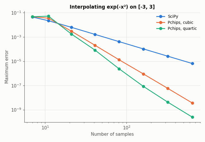
8
|
+
to use, copy, modify, merge, publish, distribute, sublicense, and/or sell
|
|
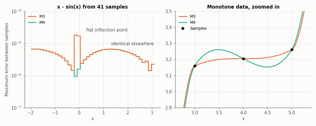
9
|
+
copies of the Software, and to permit persons to whom the Software is
|
|
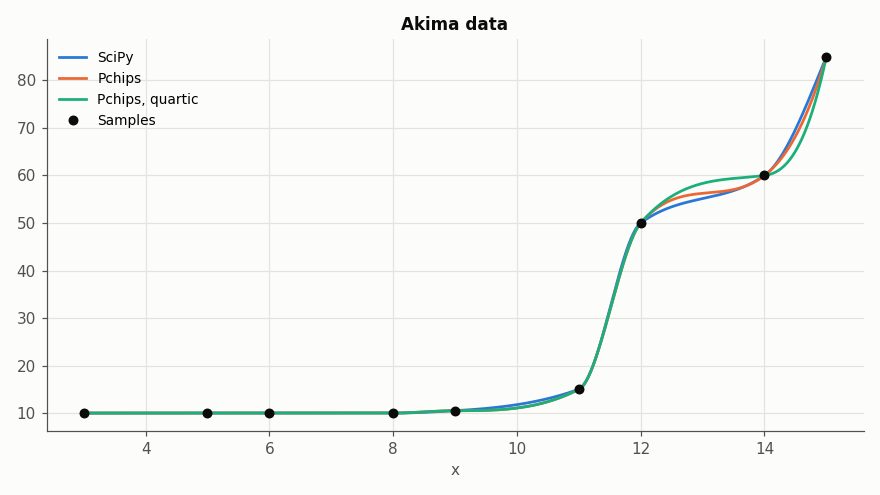
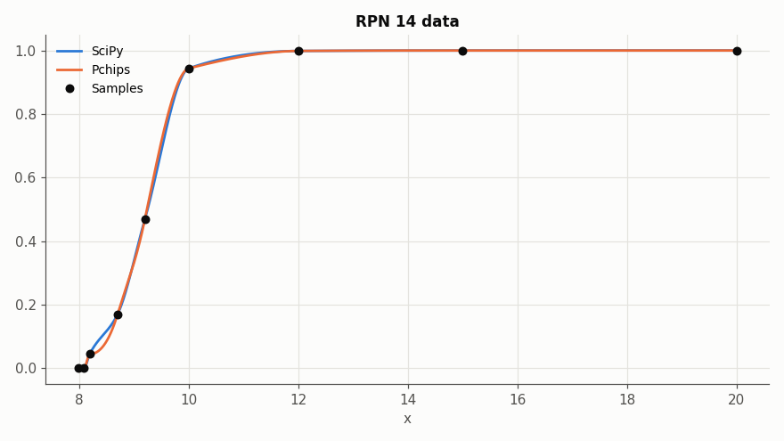
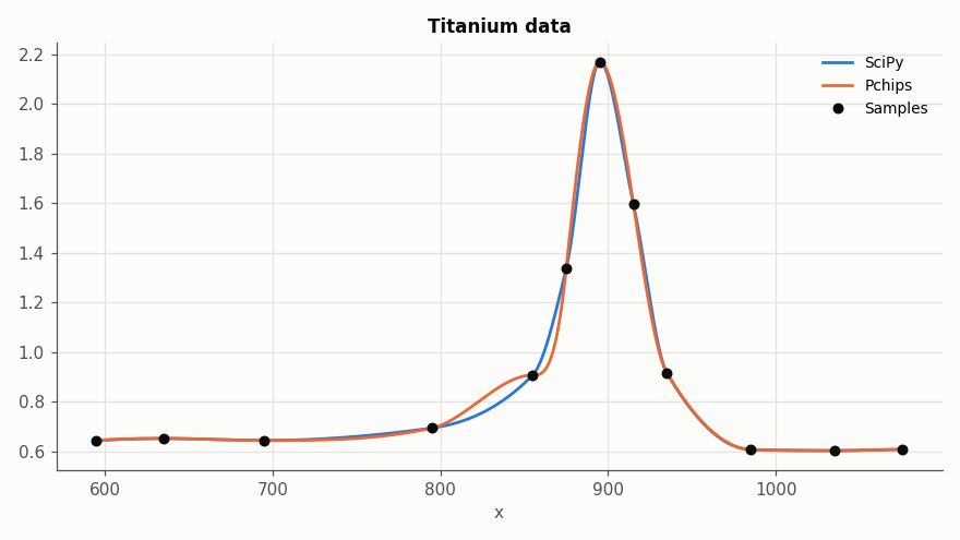
10
|
+
furnished to do so, subject to the following conditions:
|
|
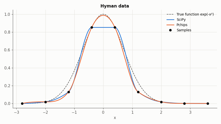
11
|
+
|
|
12
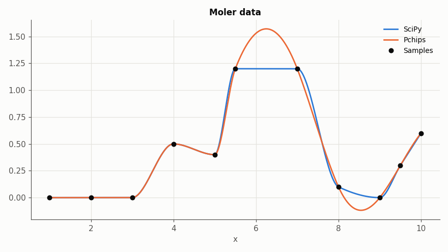
|
+
The above copyright notice and this permission notice shall be included in all
|
|
13
|
+
copies or substantial portions of the Software.
|
|
14
|
+
|
|
15
|
+
THE SOFTWARE IS PROVIDED "AS IS", WITHOUT WARRANTY OF ANY KIND, EXPRESS OR
|
|
16
|
+
IMPLIED, INCLUDING BUT NOT LIMITED TO THE WARRANTIES OF MERCHANTABILITY,
|
|
17
|
+
FITNESS FOR A PARTICULAR PURPOSE AND NONINFRINGEMENT. IN NO EVENT SHALL THE
|
|
18
|
+
AUTHORS OR COPYRIGHT HOLDERS BE LIABLE FOR ANY CLAIM, DAMAGES OR OTHER
|
|
19
|
+
LIABILITY, WHETHER IN AN ACTION OF CONTRACT, TORT OR OTHERWISE, ARISING FROM,
|
|
20
|
+
OUT OF OR IN CONNECTION WITH THE SOFTWARE OR THE USE OR OTHER DEALINGS IN THE
|
|
21
|
+
SOFTWARE.
|
pchips-1.0.0/PKG-INFO
ADDED
|
@@ -0,0 +1,241 @@
|
|
|
1
|
+
Metadata-Version: 2.5
|
|
2
|
+
Name: pchips
|
|
3
|
+
Version: 1.0.0
|
|
4
|
+
Summary: A drop-in replacement for scipy.interpolate.PchipInterpolator using H. T. Huynh's accurate monotone cubic interpolant.
|
|
5
|
+
Project-URL: Homepage, https://github.com/vglazer/pchips
|
|
6
|
+
Project-URL: Source, https://github.com/vglazer/pchips
|
|
7
|
+
Project-URL: Issues, https://github.com/vglazer/pchips/issues
|
|
8
|
+
Author: Victor Glazer
|
|
9
|
+
License-Expression: MIT
|
|
10
|
+
License-File: LICENSE
|
|
11
|
+
Keywords: cubic,hermite,interpolation,monotone,pchip,scipy,spline
|
|
12
|
+
Classifier: Intended Audience :: Science/Research
|
|
13
|
+
Classifier: Operating System :: OS Independent
|
|
14
|
+
Classifier: Programming Language :: Python :: 3
|
|
15
|
+
Classifier: Programming Language :: Python :: 3.10
|
|
16
|
+
Classifier: Programming Language :: Python :: 3.11
|
|
17
|
+
Classifier: Programming Language :: Python :: 3.12
|
|
18
|
+
Classifier: Programming Language :: Python :: 3.13
|
|
19
|
+
Classifier: Programming Language :: Python :: 3.14
|
|
20
|
+
Classifier: Topic :: Scientific/Engineering :: Mathematics
|
|
21
|
+
Requires-Python: >=3.10
|
|
22
|
+
Requires-Dist: numpy>=1.23.5
|
|
23
|
+
Requires-Dist: scipy>=1.10
|
|
24
|
+
Description-Content-Type: text/markdown
|
|
25
|
+
|
|
26
|
+
# Pchips
|
|
27
|
+
|
|
28
|
+
|
|
29
|
+
|
|
30
|
+
## Overview
|
|
31
|
+
|
|
32
|
+
This is a Python port, produced using [Gemini CLI](https://github.com/google-gemini/gemini-cli) in an afternoon, of the accurate monotone cubic interpolant [originally implemented in MATLAB here](https://github.com/vglazer/USRA/tree/master/interpolation). It was then refined using [Claude Code](https://claude.com/claude-code): checked against Huynh's paper (which turned up and fixed two bugs in the M4 constraint inherited from the MATLAB original), turned into a drop-in replacement for SciPy's [PchipInterpolator](https://docs.scipy.org/doc/scipy/reference/generated/scipy.interpolate.PchipInterpolator.html), vectorized, and given a more thorough test suite.
|
|
33
|
+
|
|
34
|
+
All the logic is in [interpolate.py](https://github.com/vglazer/pchips/blob/main/src/pchips/interpolate.py). The [tests](https://github.com/vglazer/pchips/tree/main/tests) compare it to SciPy, check the guarantees from Huynh's paper and generate comparison plots. [test_scipy_suite.py](https://github.com/vglazer/pchips/blob/main/tests/test_scipy_suite.py) runs SciPy's own `PchipInterpolator` tests against it.
|
|
35
|
+
|
|
36
|
+
The algorithm, due to [H. T. Huynh](https://scholar.google.com/citations?user=ZXhGCtwAAAAJ&hl=en), is described in this [NASA Technical Memo](https://ntrs.nasa.gov/citations/19910011517), which is self-contained and quite readable. A nearly identical version was later published in the [SIAM Journal on Numerical Analysis](https://epubs.siam.org/doi/10.1137/0730004).
|
|
37
|
+
|
|
38
|
+
## Gallery
|
|
39
|
+
|
|
40
|
+
These plots show where Pchips differs from SciPy's `PchipInterpolator`, and how its options differ from each other. They are generated by [make_gallery.py](https://github.com/vglazer/pchips/blob/main/scripts/make_gallery.py): run `uv run python scripts/make_gallery.py` to regenerate them.
|
|
41
|
+
|
|
42
|
+
### Preserving versus imposing monotonicity
|
|
43
|
+
|
|
44
|
+
#### Peaks and troughs
|
|
45
|
+
|
|
46
|
+
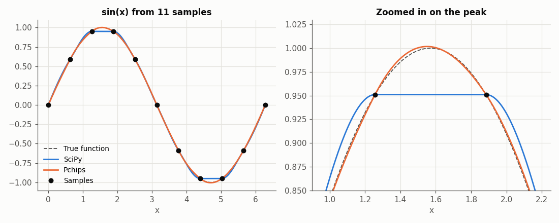
In the plot at the top of this page, the peak of sin(x) falls exactly between two samples with equal values, so the data are flat there. SciPy's interpolant _imposes_ monotonicity by setting the derivative to zero at both samples, which cuts the peak off flat at 0.951. Pchips only _preserves_ monotonicity where the data are monotone, so it follows the curve up to 1.002, close to the true peak of 1. The maximum error is 0.049 for SciPy and 0.0055 for Pchips.
|
|
47
|
+
|
|
48
|
+
#### Accuracy as the samples get denser
|
|
49
|
+
|
|
50
|
+
|
|
51
|
+
|
|
52
|
+
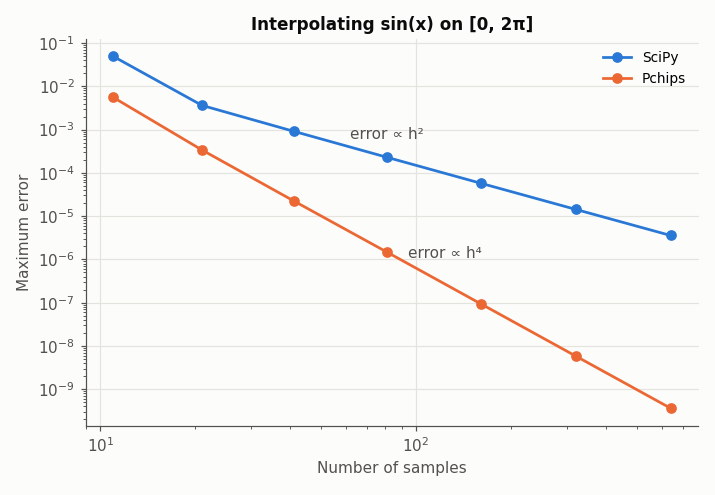
Flattening every peak and trough limits SciPy's interpolant to O(h²) accuracy, while Pchips is O(h⁴): doubling the number of samples cuts SciPy's error by a factor of 4, and Pchips' by 16. With 641 samples, the maximum error is 3.6e-6 for SciPy and 3.6e-10 for Pchips.
|
|
53
|
+
|
|
54
|
+
#### Monotone data stay monotone
|
|
55
|
+
|
|
56
|
+
|
|
57
|
+
|
|
58
|
+
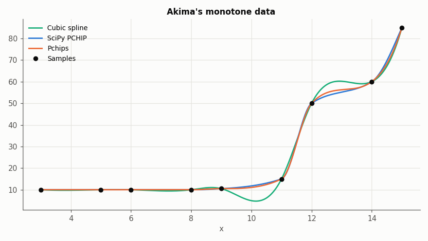
On monotone data, both PCHIPs give a monotone interpolant with no overshoot, unlike a cubic spline, which dips to 4.74 on data which never go below 10 and bulges above 60 between the samples at 50 and 60.
|
|
59
|
+
|
|
60
|
+
#### The price: overshoot on rough data
|
|
61
|
+
|
|
62
|
+
|
|
63
|
+
|
|
64
|
+
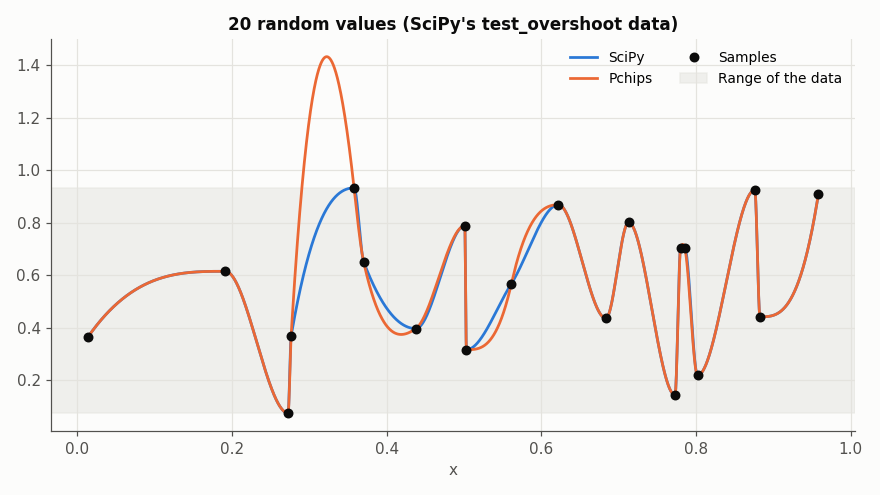
Relaxing the constraint near peaks and troughs means Pchips can overshoot the data there. On smooth data the overshoot is small and usually closer to the truth, as in the plot at the top. On rough data it can be large: on these 20 random values in [0.08, 0.93], from SciPy's own `test_overshoot`, Pchips reaches 1.43, while SciPy stays within the range of the data.
|
|
65
|
+
|
|
66
|
+
### Cubic versus quartic
|
|
67
|
+
|
|
68
|
+
|
|
69
|
+
|
|
70
|
+
Both derivative approximations give an O(h⁴) interpolant, but the quartic one has a smaller error constant: with 641 samples of e^(−x²), the maximum error is 3.6e-9 with cubic and 2.5e-10 with quartic (and 6.5e-6 with SciPy). With very few samples, however, quartic can be worse, since it relies on the data being smooth over five neighbouring samples rather than four: with 11 samples, the error is 3.6e-2 with cubic and 5.2e-2 with quartic. Use quartic once the samples resolve the shape of the data.
|
|
71
|
+
|
|
72
|
+
### M3 versus M4
|
|
73
|
+
|
|
74
|
+
|
|
75
|
+
|
|
76
|
+
**Left**: on smooth, well-sampled data, M3 and M4 give the same interpolant except near a flat inflection point, where the slope of a monotone function drops to zero between samples, as for x - sin(x) at x = 0. There, M3 clips the derivatives to keep the interpolant monotone and loses accuracy: with 41 samples, the maximum error is 1.8e-5 with M3 and 6.7e-6 with M4.
|
|
77
|
+
|
|
78
|
+
**Right**: the price of M4. To stay fourth-order accurate, M4 allows derivatives which can make the interpolant non-monotone on rough monotone data. On this data set, which increases at every sample, the M4 interpolant decreases by 0.11 between x = 3.5 and x = 4.5, while the M3 interpolant stays monotone.
|
|
79
|
+
|
|
80
|
+
### Classic data sets
|
|
81
|
+
|
|
82
|
+
These are the data sets in [data](https://github.com/vglazer/pchips/tree/main/data), which the tests also use. Each plot compares SciPy with Pchips' default settings (and, for Akima's data, the quartic approximation too).
|
|
83
|
+
|
|
84
|
+
#### Hyman
|
|
85
|
+
|
|
86
|
+
|
|
87
|
+
|
|
88
|
+
Nine samples of e^(−x²), with the peak between the samples at ±0.4. SciPy cuts the peak off flat at 0.852, an error of 0.148, while Pchips reaches 0.988, an error of 0.012. Away from the peak, nine samples are too few for either interpolant to follow the curve closely, and Pchips is off by up to 0.128 at x = 1.06.
|
|
89
|
+
|
|
90
|
+
#### Moler
|
|
91
|
+
|
|
92
|
+
|
|
93
|
+
|
|
94
|
+
Rough, non-monotone data with plateaus and sharp turns. SciPy stays within the data, flat across the plateau at 1.2. Pchips treats the two samples at 1.2 as either side of a peak and rounds it off up to 1.57, then dips to -0.118 between the samples at 0.1 and 0. This is the overshoot described in [Reasons not to switch](https://github.com/vglazer/pchips#reasons-not-to-switch): if the plateau and the zero floor are real features of the data, SciPy is the better choice here.
|
|
95
|
+
|
|
96
|
+
#### Akima
|
|
97
|
+
|
|
98
|
+
|
|
99
|
+
|
|
100
|
+
Monotone data with a sharp rise, one of the test cases in Huynh's paper. All three interpolants are monotone and stay within the data. SciPy and Pchips' default differ by at most 1.8, on the final rise from 60 to 85. The quartic approximation, which draws on more neighbouring samples, stands out between the samples at 50 and 60: it levels off close to 60 (59.4 at x = 13.5, against 57.0 and 56.8), then rises more steeply to 85. (See [above](https://github.com/vglazer/pchips#monotone-data-stay-monotone) for a cubic spline on the same data.)
|
|
101
|
+
|
|
102
|
+
#### RPN 14
|
|
103
|
+
|
|
104
|
+
|
|
105
|
+
|
|
106
|
+
Monotone data which rise steeply and then level off, from Fritsch and Carlson's paper on monotone interpolation, and the other test case in Huynh's paper. SciPy and Pchips are both monotone and differ by at most 0.036, mostly near the bottom of the rise.
|
|
107
|
+
|
|
108
|
+
#### Titanium
|
|
109
|
+
|
|
110
|
+
|
|
111
|
+
|
|
112
|
+
A sharp peak which happens to fall on a sample, so neither interpolant overshoots it, and both stay within the data. They differ by at most 0.12, at the foot of the peak. Pchips is flat for a moment at the sample at x = 855: its derivative estimate there came out with the wrong sign for the rising data, so the monotonicity constraint set it to zero.
|
|
113
|
+
|
|
114
|
+
## Installation
|
|
115
|
+
|
|
116
|
+
Pchips requires Python 3.10 or later, NumPy 1.23.5 or later and SciPy 1.10 or later. It is not on PyPI, so install it from GitHub:
|
|
117
|
+
|
|
118
|
+
```sh
|
|
119
|
+
pip install git+https://github.com/vglazer/pchips
|
|
120
|
+
# or
|
|
121
|
+
uv add git+https://github.com/vglazer/pchips
|
|
122
|
+
```
|
|
123
|
+
|
|
124
|
+
## Usage
|
|
125
|
+
|
|
126
|
+
Change the import and leave everything else as it is:
|
|
127
|
+
|
|
128
|
+
```python
|
|
129
|
+
# from scipy.interpolate import PchipInterpolator, pchip_interpolate
|
|
130
|
+
from pchips import PchipInterpolator, pchip_interpolate
|
|
131
|
+
|
|
132
|
+
interp = PchipInterpolator(x, y) # also axis=..., extrapolate=...
|
|
133
|
+
interp(u) # also interp(u, nu=1)
|
|
134
|
+
interp.derivative(), interp.antiderivative(), interp.integrate(a, b), interp.roots()
|
|
135
|
+
```
|
|
136
|
+
|
|
137
|
+
`PchipInterpolator` has the same signature and input validation as SciPy's, and like SciPy's version it is a [CubicHermiteSpline](https://docs.scipy.org/doc/scipy/reference/generated/scipy.interpolate.CubicHermiteSpline.html), so it has the same methods, output shapes and extrapolation behavior. On top of that, two keyword-only options select the variant of Huynh's method:
|
|
138
|
+
|
|
139
|
+
- `approx_order`: `'cubic'` (default) or `'quartic'`, the derivative approximation
|
|
140
|
+
- `mono_constraint`: `'M3'` (default) or `'M4'`, the monotonicity constraint
|
|
141
|
+
|
|
142
|
+
See below for when to use which. With fewer than five data points, the result is the same as SciPy's, up to rounding error.
|
|
143
|
+
|
|
144
|
+
As with SciPy, extrapolation is on by default and simply extends the first and last cubics, so the interpolant drifts away from the data quickly outside its range. Pass `extrapolate=False` to get `nan` there instead.
|
|
145
|
+
|
|
146
|
+
### Choosing between cubic and quartic
|
|
147
|
+
|
|
148
|
+
**Use `'quartic'` if your data are smooth and sampled finely enough to resolve their features, and `'cubic'`, the default, otherwise.**
|
|
149
|
+
|
|
150
|
+
Why:
|
|
151
|
+
|
|
152
|
+
- **Quartic is more accurate on well-resolved smooth data**. Both give an O(h⁴) interpolant, but the quartic derivative approximation has a smaller error constant. With 321 samples, the maximum error is 3.9e-10 instead of 5.8e-9 for sin(x), and 4.2e-9 instead of 5.8e-8 for e^(−x²)
|
|
153
|
+
- **Cubic can be more accurate on coarse data**. The quartic approximation uses five neighbouring samples instead of four, so it relies on the data being smooth over a wider stencil. With only 11 samples of e^(−x²) on [-3, 3], the maximum error is 5.2e-2 with quartic and 3.6e-2 with cubic, and the same happens with a steep tanh(5x) and Runge's function
|
|
154
|
+
- **Quartic is about 10% slower to construct**
|
|
155
|
+
|
|
156
|
+
### Choosing between M3 and M4
|
|
157
|
+
|
|
158
|
+
**Use M3, the default, unless your data are smooth samples of a monotone function whose slope drops to zero somewhere between the samples**, i.e. a flat inflection point such as x - sin(x) at x = 0 or x³ at x = 0.
|
|
159
|
+
|
|
160
|
+
Why:
|
|
161
|
+
|
|
162
|
+
- **On most data the two are identical**. For smooth, well-sampled data the constraint only kicks in near points where the slope of the data is close to zero. At peaks and troughs both constraints relax in the same way, which is what gives Pchips its accuracy there. On sin, e^(−x²), tanh, Runge's function and others, M3 and M4 give exactly the same interpolant
|
|
163
|
+
- **M4 is more accurate at flat inflection points**. M3 guarantees monotonicity by keeping the derivative at each sample between 0 and a bound computed from the neighbouring data: 3 times the smaller of the neighbouring slopes, or 1.5 times a local parabola's slope if that is larger. Near a flat inflection point, both are tiny, so this clips the derivatives and accuracy drops to roughly O(h³), and erratically so. M4 uses extra information from neighbouring cubics to allow larger derivatives there and stays O(h⁴). For x - sin(x) on [-2, 3.1] with 641 samples, the maximum error is 7.1e-10 with M3 and 1.0e-10 with M4 (see `test_m4_fourth_order_at_flat_inflection` in [test_vs_scipy.py](https://github.com/vglazer/pchips/blob/main/tests/test_vs_scipy.py)). For x³, M4 is exact while M3 is not. If the flat point happens to be one of the samples, the two agree again
|
|
164
|
+
- **M4 weakens the monotonicity guarantee**. Fourth-order accuracy is incompatible with monotonicity in general: there are monotone data which lie on a non-monotone cubic, and M4 reproduces the cubic. Huynh therefore only guarantees a monotone interpolant where the data are "q-monotone" (Theorem 3 in the paper), and in the two intervals at either end. On rough monotone data this matters: in 300 random monotone datasets, M4 gave an interpolant which decreases somewhere in 82 (equally spaced samples) and 141 (unequally spaced samples) of them, while M3 never did
|
|
165
|
+
- **M4 is about 1.4-1.6 times slower to construct**
|
|
166
|
+
|
|
167
|
+
So if your data are noisy or irregular, or a monotone result is a hard requirement, stick with M3. If they are smooth and you need the extra accuracy near flat inflection points, use M4, and check the result for monotonicity if that matters.
|
|
168
|
+
|
|
169
|
+
## Should you switch from SciPy?
|
|
170
|
+
|
|
171
|
+
In short: switch if your data come from a smooth underlying function and accuracy matters, especially near peaks and troughs. Stay with SciPy if your code relies on the interpolant never leaving the range of the data.
|
|
172
|
+
|
|
173
|
+
### Reasons to switch
|
|
174
|
+
|
|
175
|
+
- **Much higher accuracy near local extrema**. SciPy's interpolant flattens out at every local maximum and minimum, which makes it only O(h²) accurate there. Pchips is O(h⁴) there too, and everywhere else, except at flat inflection points with the default M3 constraint (see above). Here is the maximum error with 321 equally spaced samples (see `test_convergence_vs_scipy` in [test_vs_scipy.py](https://github.com/vglazer/pchips/blob/main/tests/test_vs_scipy.py)):
|
|
176
|
+
|
|
177
|
+
| Function | SciPy | Pchips (default) | Pchips (`approx_order='quartic'`) |
|
|
178
|
+
| --- | --- | --- | --- |
|
|
179
|
+
| sin(x) on [0, 2π] | 1.4e-5 | 5.8e-9 | 3.9e-10 |
|
|
180
|
+
| e^(−x²) on [-3, 3] | 2.6e-5 | 5.8e-8 | 4.2e-9 |
|
|
181
|
+
| tanh(x) on [-3, 3] (no extrema) | 2.1e-7 | 1.3e-8 | 1.4e-9 |
|
|
182
|
+
|
|
183
|
+
Put differently, Pchips with 41 samples of sin(x) (2.2e-5) is nearly as accurate as SciPy with 321 (1.4e-5), and the gap grows as you add samples
|
|
184
|
+
- **The same monotonicity guarantee**. With the default M3 constraint, monotone data give a monotone interpolant, just like SciPy's
|
|
185
|
+
- **Low-degree polynomials are reproduced exactly**, along with their derivatives and integrals. Quadratics always are, and so are cubics with M4. With the default M3, cubics are exact where they are monotone, but not across a flat inflection point, nor near their extrema when the samples are coarse. SciPy's interpolant is not exact even for quadratics
|
|
186
|
+
- **Switching is a one-line change**. Only the import changes, and SciPy's own `PchipInterpolator` tests pass, apart from two: one checks that the interpolant never overshoots, which Huynh's method deliberately gives up, and the other checks the exact values of SciPy's method (see [test_scipy_suite.py](https://github.com/vglazer/pchips/blob/main/tests/test_scipy_suite.py))
|
|
187
|
+
|
|
188
|
+
### Reasons not to switch
|
|
189
|
+
|
|
190
|
+
- **The interpolant may overshoot the data near strict local extrema**. This is the price of accuracy: between any two neighbouring samples, SciPy's interpolant always stays between their values, which is exactly what limits it to O(h²) at peaks and troughs. How far Pchips overshoots depends on how smooth the data are:
|
|
191
|
+
- **On smooth data the overshoot is small**, and usually closer to the truth, since the underlying function typically peaks between samples. For example, data with a minimum of 0.02 can give an interpolant which dips to -0.004
|
|
192
|
+
- **On rough data it can be large**. In SciPy's `test_overshoot`, which interpolates 20 random values (one of the two expected failures in [test_scipy_suite.py](https://github.com/vglazer/pchips/blob/main/tests/test_scipy_suite.py)), Pchips leaves the range of the neighbouring samples in 3 of the 19 intervals, by up to 0.50 when the data span 0.86
|
|
193
|
+
|
|
194
|
+
If that matters, e.g. for probabilities, concentrations or anything passed to `log`, stay with SciPy or clip the result
|
|
195
|
+
- **Construction is 1.3-3 times slower** (see below). This only matters if you build interpolators in a hot loop
|
|
196
|
+
- **Rough or noisy data gain little**, since the higher accuracy relies on the data being smooth
|
|
197
|
+
|
|
198
|
+
### Performance
|
|
199
|
+
|
|
200
|
+
Evaluating the interpolant, along with its derivatives and integrals, is exactly as fast as SciPy's, since both use the same `CubicHermiteSpline` code: about 0.5 ms for 100,000 points. Construction does more work, because Huynh's method uses higher-order divided differences and a more elaborate monotonicity constraint. Construction times, best of 7 runs on an Apple M3 Max with Python 3.13, NumPy 2.3 and SciPy 1.16, with the slowdown relative to SciPy in brackets:
|
|
201
|
+
|
|
202
|
+
| Data | SciPy | Pchips (default) | Pchips (`approx_order='quartic'`, `mono_constraint='M4'`) |
|
|
203
|
+
| --- | --- | --- | --- |
|
|
204
|
+
| 20 points | 0.05 ms | 0.08 ms (1.6× slower) | 0.11 ms (2.2× slower) |
|
|
205
|
+
| 1,000 points | 0.06 ms | 0.10 ms (1.6× slower) | 0.14 ms (2.3× slower) |
|
|
206
|
+
| 100,000 points | 1.3 ms | 2.3 ms (1.8× slower) | 3.7 ms (2.9× slower) |
|
|
207
|
+
| 50 points × 1,000 columns | 0.9 ms | 1.1 ms (1.3× slower) | 1.7 ms (1.9× slower) |
|
|
208
|
+
|
|
209
|
+
## Mathematical background
|
|
210
|
+
|
|
211
|
+
The mathematical background is written in LaTeX, which PyPI cannot display, so read it [on GitHub](https://github.com/vglazer/pchips#mathematical-background).
|
|
212
|
+
|
|
213
|
+
## Development
|
|
214
|
+
|
|
215
|
+
- Make sure you have [uv installed](https://docs.astral.sh/uv/getting-started/installation/)
|
|
216
|
+
- Clone the repo
|
|
217
|
+
- `cd pchips`
|
|
218
|
+
- `uv sync`
|
|
219
|
+
- `uv run pytest`
|
|
220
|
+
- Check out the comparison plots in the `plots` subdirectory
|
|
221
|
+
|
|
222
|
+
## Citation
|
|
223
|
+
|
|
224
|
+
If you use Pchips in published work, please cite Huynh's paper:
|
|
225
|
+
|
|
226
|
+
```bibtex
|
|
227
|
+
@article{huynh1993accurate,
|
|
228
|
+
author = {Huynh, Hung T.},
|
|
229
|
+
title = {Accurate Monotone Cubic Interpolation},
|
|
230
|
+
journal = {SIAM Journal on Numerical Analysis},
|
|
231
|
+
volume = {30},
|
|
232
|
+
number = {1},
|
|
233
|
+
pages = {57--100},
|
|
234
|
+
year = {1993},
|
|
235
|
+
doi = {10.1137/0730004}
|
|
236
|
+
}
|
|
237
|
+
```
|
|
238
|
+
|
|
239
|
+
## License
|
|
240
|
+
|
|
241
|
+
Pchips is released under the [MIT License](https://github.com/vglazer/pchips/blob/main/LICENSE). [test_scipy_suite.py](https://github.com/vglazer/pchips/blob/main/tests/test_scipy_suite.py) is adapted from SciPy's tests and keeps SciPy's BSD 3-Clause License, which is reproduced at the top of that file.
|
pchips-1.0.0/README.md
ADDED
|
@@ -0,0 +1,231 @@
|
|
|
1
|
+
# Pchips
|
|
2
|
+
|
|
3
|
+

|
|
4
|
+
|
|
5
|
+
## Overview
|
|
6
|
+
|
|
7
|
+
This is a Python port, produced using [Gemini CLI](https://github.com/google-gemini/gemini-cli) in an afternoon, of the accurate monotone cubic interpolant [originally implemented in MATLAB here](https://github.com/vglazer/USRA/tree/master/interpolation). It was then refined using [Claude Code](https://claude.com/claude-code): checked against Huynh's paper (which turned up and fixed two bugs in the M4 constraint inherited from the MATLAB original), turned into a drop-in replacement for SciPy's [PchipInterpolator](https://docs.scipy.org/doc/scipy/reference/generated/scipy.interpolate.PchipInterpolator.html), vectorized, and given a more thorough test suite.
|
|
8
|
+
|
|
9
|
+
All the logic is in [interpolate.py](src/pchips/interpolate.py). The [tests](tests) compare it to SciPy, check the guarantees from Huynh's paper and generate comparison plots. [test_scipy_suite.py](tests/test_scipy_suite.py) runs SciPy's own `PchipInterpolator` tests against it.
|
|
10
|
+
|
|
11
|
+
The algorithm, due to [H. T. Huynh](https://scholar.google.com/citations?user=ZXhGCtwAAAAJ&hl=en), is described in this [NASA Technical Memo](https://ntrs.nasa.gov/citations/19910011517), which is self-contained and quite readable. A nearly identical version was later published in the [SIAM Journal on Numerical Analysis](https://epubs.siam.org/doi/10.1137/0730004).
|
|
12
|
+
|
|
13
|
+
## Gallery
|
|
14
|
+
|
|
15
|
+
These plots show where Pchips differs from SciPy's `PchipInterpolator`, and how its options differ from each other. They are generated by [make_gallery.py](scripts/make_gallery.py): run `uv run python scripts/make_gallery.py` to regenerate them.
|
|
16
|
+
|
|
17
|
+
### Preserving versus imposing monotonicity
|
|
18
|
+
|
|
19
|
+
#### Peaks and troughs
|
|
20
|
+
|
|
21
|
+
In the plot at the top of this page, the peak of $\sin(x)$ falls exactly between two samples with equal values, so the data are flat there. SciPy's interpolant _imposes_ monotonicity by setting the derivative to zero at both samples, which cuts the peak off flat at 0.951. Pchips only _preserves_ monotonicity where the data are monotone, so it follows the curve up to 1.002, close to the true peak of 1. The maximum error is 0.049 for SciPy and 0.0055 for Pchips.
|
|
22
|
+
|
|
23
|
+
#### Accuracy as the samples get denser
|
|
24
|
+
|
|
25
|
+

|
|
26
|
+
|
|
27
|
+
Flattening every peak and trough limits SciPy's interpolant to $O(h^2)$ accuracy, while Pchips is $O(h^4)$: doubling the number of samples cuts SciPy's error by a factor of 4, and Pchips' by 16. With 641 samples, the maximum error is 3.6e-6 for SciPy and 3.6e-10 for Pchips.
|
|
28
|
+
|
|
29
|
+
#### Monotone data stay monotone
|
|
30
|
+
|
|
31
|
+

|
|
32
|
+
|
|
33
|
+
On monotone data, both PCHIPs give a monotone interpolant with no overshoot, unlike a cubic spline, which dips to 4.74 on data which never go below 10 and bulges above 60 between the samples at 50 and 60.
|
|
34
|
+
|
|
35
|
+
#### The price: overshoot on rough data
|
|
36
|
+
|
|
37
|
+

|
|
38
|
+
|
|
39
|
+
Relaxing the constraint near peaks and troughs means Pchips can overshoot the data there. On smooth data the overshoot is small and usually closer to the truth, as in the plot at the top. On rough data it can be large: on these 20 random values in [0.08, 0.93], from SciPy's own `test_overshoot`, Pchips reaches 1.43, while SciPy stays within the range of the data.
|
|
40
|
+
|
|
41
|
+
### Cubic versus quartic
|
|
42
|
+
|
|
43
|
+

|
|
44
|
+
|
|
45
|
+
Both derivative approximations give an $O(h^4)$ interpolant, but the quartic one has a smaller error constant: with 641 samples of $e^{-x^2}$, the maximum error is 3.6e-9 with cubic and 2.5e-10 with quartic (and 6.5e-6 with SciPy). With very few samples, however, quartic can be worse, since it relies on the data being smooth over five neighbouring samples rather than four: with 11 samples, the error is 3.6e-2 with cubic and 5.2e-2 with quartic. Use quartic once the samples resolve the shape of the data.
|
|
46
|
+
|
|
47
|
+
### M3 versus M4
|
|
48
|
+
|
|
49
|
+

|
|
50
|
+
|
|
51
|
+
**Left**: on smooth, well-sampled data, M3 and M4 give the same interpolant except near a flat inflection point, where the slope of a monotone function drops to zero between samples, as for $x - \sin(x)$ at $x = 0$. There, M3 clips the derivatives to keep the interpolant monotone and loses accuracy: with 41 samples, the maximum error is 1.8e-5 with M3 and 6.7e-6 with M4.
|
|
52
|
+
|
|
53
|
+
**Right**: the price of M4. To stay fourth-order accurate, M4 allows derivatives which can make the interpolant non-monotone on rough monotone data. On this data set, which increases at every sample, the M4 interpolant decreases by 0.11 between $x = 3.5$ and $x = 4.5$, while the M3 interpolant stays monotone.
|
|
54
|
+
|
|
55
|
+
### Classic data sets
|
|
56
|
+
|
|
57
|
+
These are the data sets in [data](data), which the tests also use. Each plot compares SciPy with Pchips' default settings (and, for Akima's data, the quartic approximation too).
|
|
58
|
+
|
|
59
|
+
#### Hyman
|
|
60
|
+
|
|
61
|
+

|
|
62
|
+
|
|
63
|
+
Nine samples of $e^{-x^2}$, with the peak between the samples at $\pm 0.4$. SciPy cuts the peak off flat at 0.852, an error of 0.148, while Pchips reaches 0.988, an error of 0.012. Away from the peak, nine samples are too few for either interpolant to follow the curve closely, and Pchips is off by up to 0.128 at $x = 1.06$.
|
|
64
|
+
|
|
65
|
+
#### Moler
|
|
66
|
+
|
|
67
|
+

|
|
68
|
+
|
|
69
|
+
Rough, non-monotone data with plateaus and sharp turns. SciPy stays within the data, flat across the plateau at 1.2. Pchips treats the two samples at 1.2 as either side of a peak and rounds it off up to 1.57, then dips to -0.118 between the samples at 0.1 and 0. This is the overshoot described in [Reasons not to switch](#reasons-not-to-switch): if the plateau and the zero floor are real features of the data, SciPy is the better choice here.
|
|
70
|
+
|
|
71
|
+
#### Akima
|
|
72
|
+
|
|
73
|
+

|
|
74
|
+
|
|
75
|
+
Monotone data with a sharp rise, one of the test cases in Huynh's paper. All three interpolants are monotone and stay within the data. SciPy and Pchips' default differ by at most 1.8, on the final rise from 60 to 85. The quartic approximation, which draws on more neighbouring samples, stands out between the samples at 50 and 60: it levels off close to 60 (59.4 at $x = 13.5$, against 57.0 and 56.8), then rises more steeply to 85. (See [above](#monotone-data-stay-monotone) for a cubic spline on the same data.)
|
|
76
|
+
|
|
77
|
+
#### RPN 14
|
|
78
|
+
|
|
79
|
+

|
|
80
|
+
|
|
81
|
+
Monotone data which rise steeply and then level off, from Fritsch and Carlson's paper on monotone interpolation, and the other test case in Huynh's paper. SciPy and Pchips are both monotone and differ by at most 0.036, mostly near the bottom of the rise.
|
|
82
|
+
|
|
83
|
+
#### Titanium
|
|
84
|
+
|
|
85
|
+

|
|
86
|
+
|
|
87
|
+
A sharp peak which happens to fall on a sample, so neither interpolant overshoots it, and both stay within the data. They differ by at most 0.12, at the foot of the peak. Pchips is flat for a moment at the sample at $x = 855$: its derivative estimate there came out with the wrong sign for the rising data, so the monotonicity constraint set it to zero.
|
|
88
|
+
|
|
89
|
+
## Installation
|
|
90
|
+
|
|
91
|
+
Pchips requires Python 3.10 or later, NumPy 1.23.5 or later and SciPy 1.10 or later. It is not on PyPI, so install it from GitHub:
|
|
92
|
+
|
|
93
|
+
```sh
|
|
94
|
+
pip install git+https://github.com/vglazer/pchips
|
|
95
|
+
# or
|
|
96
|
+
uv add git+https://github.com/vglazer/pchips
|
|
97
|
+
```
|
|
98
|
+
|
|
99
|
+
## Usage
|
|
100
|
+
|
|
101
|
+
Change the import and leave everything else as it is:
|
|
102
|
+
|
|
103
|
+
```python
|
|
104
|
+
# from scipy.interpolate import PchipInterpolator, pchip_interpolate
|
|
105
|
+
from pchips import PchipInterpolator, pchip_interpolate
|
|
106
|
+
|
|
107
|
+
interp = PchipInterpolator(x, y) # also axis=..., extrapolate=...
|
|
108
|
+
interp(u) # also interp(u, nu=1)
|
|
109
|
+
interp.derivative(), interp.antiderivative(), interp.integrate(a, b), interp.roots()
|
|
110
|
+
```
|
|
111
|
+
|
|
112
|
+
`PchipInterpolator` has the same signature and input validation as SciPy's, and like SciPy's version it is a [CubicHermiteSpline](https://docs.scipy.org/doc/scipy/reference/generated/scipy.interpolate.CubicHermiteSpline.html), so it has the same methods, output shapes and extrapolation behavior. On top of that, two keyword-only options select the variant of Huynh's method:
|
|
113
|
+
|
|
114
|
+
- `approx_order`: `'cubic'` (default) or `'quartic'`, the derivative approximation
|
|
115
|
+
- `mono_constraint`: `'M3'` (default) or `'M4'`, the monotonicity constraint
|
|
116
|
+
|
|
117
|
+
See below for when to use which. With fewer than five data points, the result is the same as SciPy's, up to rounding error.
|
|
118
|
+
|
|
119
|
+
As with SciPy, extrapolation is on by default and simply extends the first and last cubics, so the interpolant drifts away from the data quickly outside its range. Pass `extrapolate=False` to get `nan` there instead.
|
|
120
|
+
|
|
121
|
+
### Choosing between cubic and quartic
|
|
122
|
+
|
|
123
|
+
**Use `'quartic'` if your data are smooth and sampled finely enough to resolve their features, and `'cubic'`, the default, otherwise.**
|
|
124
|
+
|
|
125
|
+
Why:
|
|
126
|
+
|
|
127
|
+
- **Quartic is more accurate on well-resolved smooth data**. Both give an $O(h^4)$ interpolant, but the quartic derivative approximation has a smaller error constant. With 321 samples, the maximum error is 3.9e-10 instead of 5.8e-9 for $\sin(x)$, and 4.2e-9 instead of 5.8e-8 for $e^{-x^2}$
|
|
128
|
+
- **Cubic can be more accurate on coarse data**. The quartic approximation uses five neighbouring samples instead of four, so it relies on the data being smooth over a wider stencil. With only 11 samples of $e^{-x^2}$ on $[-3, 3]$, the maximum error is 5.2e-2 with quartic and 3.6e-2 with cubic, and the same happens with a steep $\tanh(5x)$ and Runge's function
|
|
129
|
+
- **Quartic is about 10% slower to construct**
|
|
130
|
+
|
|
131
|
+
### Choosing between M3 and M4
|
|
132
|
+
|
|
133
|
+
**Use M3, the default, unless your data are smooth samples of a monotone function whose slope drops to zero somewhere between the samples**, i.e. a flat inflection point such as $x - \sin(x)$ at $x = 0$ or $x^3$ at $x = 0$.
|
|
134
|
+
|
|
135
|
+
Why:
|
|
136
|
+
|
|
137
|
+
- **On most data the two are identical**. For smooth, well-sampled data the constraint only kicks in near points where the slope of the data is close to zero. At peaks and troughs both constraints relax in the same way, which is what gives Pchips its accuracy there. On $\sin$, $e^{-x^2}$, $\tanh$, Runge's function and others, M3 and M4 give exactly the same interpolant
|
|
138
|
+
- **M4 is more accurate at flat inflection points**. M3 guarantees monotonicity by keeping the derivative at each sample between 0 and a bound computed from the neighbouring data: 3 times the smaller of the neighbouring slopes, or 1.5 times a local parabola's slope if that is larger. Near a flat inflection point, both are tiny, so this clips the derivatives and accuracy drops to roughly $O(h^3)$, and erratically so. M4 uses extra information from neighbouring cubics to allow larger derivatives there and stays $O(h^4)$. For $x - \sin(x)$ on $[-2, 3.1]$ with 641 samples, the maximum error is 7.1e-10 with M3 and 1.0e-10 with M4 (see `test_m4_fourth_order_at_flat_inflection` in [test_vs_scipy.py](tests/test_vs_scipy.py)). For $x^3$, M4 is exact while M3 is not. If the flat point happens to be one of the samples, the two agree again
|
|
139
|
+
- **M4 weakens the monotonicity guarantee**. Fourth-order accuracy is incompatible with monotonicity in general: there are monotone data which lie on a non-monotone cubic, and M4 reproduces the cubic. Huynh therefore only guarantees a monotone interpolant where the data are "q-monotone" (Theorem 3 in the paper), and in the two intervals at either end. On rough monotone data this matters: in 300 random monotone datasets, M4 gave an interpolant which decreases somewhere in 82 (equally spaced samples) and 141 (unequally spaced samples) of them, while M3 never did
|
|
140
|
+
- **M4 is about 1.4-1.6 times slower to construct**
|
|
141
|
+
|
|
142
|
+
So if your data are noisy or irregular, or a monotone result is a hard requirement, stick with M3. If they are smooth and you need the extra accuracy near flat inflection points, use M4, and check the result for monotonicity if that matters.
|
|
143
|
+
|
|
144
|
+
## Should you switch from SciPy?
|
|
145
|
+
|
|
146
|
+
In short: switch if your data come from a smooth underlying function and accuracy matters, especially near peaks and troughs. Stay with SciPy if your code relies on the interpolant never leaving the range of the data.
|
|
147
|
+
|
|
148
|
+
### Reasons to switch
|
|
149
|
+
|
|
150
|
+
- **Much higher accuracy near local extrema**. SciPy's interpolant flattens out at every local maximum and minimum, which makes it only $O(h^2)$ accurate there. Pchips is $O(h^4)$ there too, and everywhere else, except at flat inflection points with the default M3 constraint (see above). Here is the maximum error with 321 equally spaced samples (see `test_convergence_vs_scipy` in [test_vs_scipy.py](tests/test_vs_scipy.py)):
|
|
151
|
+
|
|
152
|
+
| Function | SciPy | Pchips (default) | Pchips (`approx_order='quartic'`) |
|
|
153
|
+
| --- | --- | --- | --- |
|
|
154
|
+
| $\sin(x)$ on $[0, 2\pi]$ | 1.4e-5 | 5.8e-9 | 3.9e-10 |
|
|
155
|
+
| $e^{-x^2}$ on $[-3, 3]$ | 2.6e-5 | 5.8e-8 | 4.2e-9 |
|
|
156
|
+
| $\tanh(x)$ on $[-3, 3]$ (no extrema) | 2.1e-7 | 1.3e-8 | 1.4e-9 |
|
|
157
|
+
|
|
158
|
+
Put differently, Pchips with 41 samples of $\sin(x)$ (2.2e-5) is nearly as accurate as SciPy with 321 (1.4e-5), and the gap grows as you add samples
|
|
159
|
+
- **The same monotonicity guarantee**. With the default M3 constraint, monotone data give a monotone interpolant, just like SciPy's
|
|
160
|
+
- **Low-degree polynomials are reproduced exactly**, along with their derivatives and integrals. Quadratics always are, and so are cubics with M4. With the default M3, cubics are exact where they are monotone, but not across a flat inflection point, nor near their extrema when the samples are coarse. SciPy's interpolant is not exact even for quadratics
|
|
161
|
+
- **Switching is a one-line change**. Only the import changes, and SciPy's own `PchipInterpolator` tests pass, apart from two: one checks that the interpolant never overshoots, which Huynh's method deliberately gives up, and the other checks the exact values of SciPy's method (see [test_scipy_suite.py](tests/test_scipy_suite.py))
|
|
162
|
+
|
|
163
|
+
### Reasons not to switch
|
|
164
|
+
|
|
165
|
+
- **The interpolant may overshoot the data near strict local extrema**. This is the price of accuracy: between any two neighbouring samples, SciPy's interpolant always stays between their values, which is exactly what limits it to $O(h^2)$ at peaks and troughs. How far Pchips overshoots depends on how smooth the data are:
|
|
166
|
+
- **On smooth data the overshoot is small**, and usually closer to the truth, since the underlying function typically peaks between samples. For example, data with a minimum of 0.02 can give an interpolant which dips to -0.004
|
|
167
|
+
- **On rough data it can be large**. In SciPy's `test_overshoot`, which interpolates 20 random values (one of the two expected failures in [test_scipy_suite.py](tests/test_scipy_suite.py)), Pchips leaves the range of the neighbouring samples in 3 of the 19 intervals, by up to 0.50 when the data span 0.86
|
|
168
|
+
|
|
169
|
+
If that matters, e.g. for probabilities, concentrations or anything passed to `log`, stay with SciPy or clip the result
|
|
170
|
+
- **Construction is 1.3-3 times slower** (see below). This only matters if you build interpolators in a hot loop
|
|
171
|
+
- **Rough or noisy data gain little**, since the higher accuracy relies on the data being smooth
|
|
172
|
+
|
|
173
|
+
### Performance
|
|
174
|
+
|
|
175
|
+
Evaluating the interpolant, along with its derivatives and integrals, is exactly as fast as SciPy's, since both use the same `CubicHermiteSpline` code: about 0.5 ms for 100,000 points. Construction does more work, because Huynh's method uses higher-order divided differences and a more elaborate monotonicity constraint. Construction times, best of 7 runs on an Apple M3 Max with Python 3.13, NumPy 2.3 and SciPy 1.16, with the slowdown relative to SciPy in brackets:
|
|
176
|
+
|
|
177
|
+
| Data | SciPy | Pchips (default) | Pchips (`approx_order='quartic'`, `mono_constraint='M4'`) |
|
|
178
|
+
| --- | --- | --- | --- |
|
|
179
|
+
| 20 points | 0.05 ms | 0.08 ms (1.6× slower) | 0.11 ms (2.2× slower) |
|
|
180
|
+
| 1,000 points | 0.06 ms | 0.10 ms (1.6× slower) | 0.14 ms (2.3× slower) |
|
|
181
|
+
| 100,000 points | 1.3 ms | 2.3 ms (1.8× slower) | 3.7 ms (2.9× slower) |
|
|
182
|
+
| 50 points × 1,000 columns | 0.9 ms | 1.1 ms (1.3× slower) | 1.7 ms (1.9× slower) |
|
|
183
|
+
|
|
184
|
+
## Mathematical background
|
|
185
|
+
|
|
186
|
+
- Say that you have a bunch of discrete samples $\{(x_i, y_i)\}_{i = 0}^{n}$ which you want to interpolate on using some nice function $f: \mathbb{R} \rightarrow \mathbb{R}$ such that $f(x_i) = y_i, 0 \leq i \leq n$
|
|
187
|
+
- [Cubic splines](https://en.wikiversity.org/wiki/Cubic_Spline_Interpolation) are one popular option. They are 4th order accurate (i.e. the error term is $O(h^4)$ ) and quite smooth:
|
|
188
|
+
- Their first derivative $f'$ is not only continuous, but also differentiable (i.e. $f \in C^2$)
|
|
189
|
+
- However, cubic splines may "wiggle" by "overshooting" and "undershooting" the data. This is not visually pleasing and may be problematic for certain applications
|
|
190
|
+
- An alternative approach is to construct a [Hermite spline](https://en.wikipedia.org/wiki/Cubic_Hermite_spline), which will match not only the data but also its first derivative:
|
|
191
|
+
- That is, we also have $f'(x_i) = \hat{f'}(x_i), 0 \leq i \leq n$, where $\hat{f'}$ is the approximate derivative of the function sampled to generate the data, produced using e.g. [Newton interpolation](https://en.wikipedia.org/wiki/Polynomial_interpolation#Newton_Interpolation)
|
|
192
|
+
- If $\hat{f'}$ is 3rd-order accurate or higher then $f$ is 4th-order accurate, as with cubic splines. You give up some smoothness, though: while $f'$ is still continuous, it is no longer differentiable (i.e. $f \in C^1$)
|
|
193
|
+
- Moreover, **Hermite interpolants are still not guaranteed to preserve monotonicity**. Meaning, they may be increasing in regions where the data is decreasing and vice versa
|
|
194
|
+
- A number of approaches have been proposed for dealing with this, but they generally trade away accuracy in order to preserve monotonicity. For example, [PchipInterpolator](https://docs.scipy.org/doc/scipy/reference/generated/scipy.interpolate.PchipInterpolator.html) uses the method from [Fritsch and Butland](https://epubs.siam.org/doi/10.1137/0905021), which is only 2nd order accurate in general (i.e. no better than linear interpolation):
|
|
195
|
+
- **Intuitively, the issue is that the interpolant _imposes_ monotonicity on the data rather than simply _preserving_ it**
|
|
196
|
+
- This results in "slicing" near local maxima and minima, causing accuracy to degrade
|
|
197
|
+
- The "Monotone Convex" spline introduced by [Hagan and West](https://www.deriscope.com/docs/Hagan_West_curves_AMF.pdf) in the context of forward curve construction also suffers from this problem
|
|
198
|
+
- The modified Akima or ["Makima" interpolant](https://blogs.mathworks.com/cleve/2019/04/29/makima-piecewise-cubic-interpolation/), which is one of the variants supported by SciPy's [Akima1DInterpolator](https://docs.scipy.org/doc/scipy/reference/generated/scipy.interpolate.Akima1DInterpolator.html#scipy.interpolate.Akima1DInterpolator), produces a spline which "appears natural" and avoids slicing for non-monotone data. However, as far as I can tell, it does not guarantee 4th order accuracy. Here is Akima's [original paper](https://dl.acm.org/doi/pdf/10.1145/321607.321609).
|
|
199
|
+
- [H.T. Huynh's interpolant](https://ntrs.nasa.gov/api/citations/19910011517/downloads/19910011517.pdf), which is implemented in [interpolate.py](src/pchips/interpolate.py), effectively relaxes the monotonicity constraint near strict local extrema:
|
|
200
|
+
- This results in an interpolant which _preserves_ monotonicity without _imposing_ it. With a 3rd-order or better approximation for $\hat{f'}$, it is $O(h^4)$ accurate, including near local extrema. With the M3 constraint it may drop to $O(h^3)$ at flat inflection points, while the M4 constraint is uniformly $O(h^4)$
|
|
201
|
+
- It's also quite natural-looking, to boot
|
|
202
|
+
|
|
203
|
+
## Development
|
|
204
|
+
|
|
205
|
+
- Make sure you have [uv installed](https://docs.astral.sh/uv/getting-started/installation/)
|
|
206
|
+
- Clone the repo
|
|
207
|
+
- `cd pchips`
|
|
208
|
+
- `uv sync`
|
|
209
|
+
- `uv run pytest`
|
|
210
|
+
- Check out the comparison plots in the `plots` subdirectory
|
|
211
|
+
|
|
212
|
+
## Citation
|
|
213
|
+
|
|
214
|
+
If you use Pchips in published work, please cite Huynh's paper:
|
|
215
|
+
|
|
216
|
+
```bibtex
|
|
217
|
+
@article{huynh1993accurate,
|
|
218
|
+
author = {Huynh, Hung T.},
|
|
219
|
+
title = {Accurate Monotone Cubic Interpolation},
|
|
220
|
+
journal = {SIAM Journal on Numerical Analysis},
|
|
221
|
+
volume = {30},
|
|
222
|
+
number = {1},
|
|
223
|
+
pages = {57--100},
|
|
224
|
+
year = {1993},
|
|
225
|
+
doi = {10.1137/0730004}
|
|
226
|
+
}
|
|
227
|
+
```
|
|
228
|
+
|
|
229
|
+
## License
|
|
230
|
+
|
|
231
|
+
Pchips is released under the [MIT License](LICENSE). [test_scipy_suite.py](tests/test_scipy_suite.py) is adapted from SciPy's tests and keeps SciPy's BSD 3-Clause License, which is reproduced at the top of that file.
|