numODEsolver 2.0.3__tar.gz → 3.1__tar.gz
This diff represents the content of publicly available package versions that have been released to one of the supported registries. The information contained in this diff is provided for informational purposes only and reflects changes between package versions as they appear in their respective public registries.
- numodesolver-3.1/PKG-INFO +152 -0
- numodesolver-3.1/README.md +122 -0
- {numodesolver-2.0.3 → numodesolver-3.1}/numODEsolver/solver.py +62 -18
- numodesolver-3.1/numODEsolver.egg-info/PKG-INFO +152 -0
- {numodesolver-2.0.3 → numodesolver-3.1}/setup.py +8 -2
- numodesolver-2.0.3/PKG-INFO +0 -75
- numodesolver-2.0.3/README.md +0 -52
- numodesolver-2.0.3/numODEsolver.egg-info/PKG-INFO +0 -75
- {numodesolver-2.0.3 → numodesolver-3.1}/LICENSE +0 -0
- {numodesolver-2.0.3 → numodesolver-3.1}/numODEsolver/__init__.py +0 -0
- {numodesolver-2.0.3 → numodesolver-3.1}/numODEsolver.egg-info/SOURCES.txt +0 -0
- {numodesolver-2.0.3 → numodesolver-3.1}/numODEsolver.egg-info/dependency_links.txt +0 -0
- {numodesolver-2.0.3 → numodesolver-3.1}/numODEsolver.egg-info/requires.txt +0 -0
- {numodesolver-2.0.3 → numodesolver-3.1}/numODEsolver.egg-info/top_level.txt +0 -0
- {numodesolver-2.0.3 → numodesolver-3.1}/setup.cfg +0 -0
|
@@ -0,0 +1,152 @@
|
|
|
1
|
+
Metadata-Version: 2.4
|
|
2
|
+
Name: numODEsolver
|
|
3
|
+
Version: 3.1
|
|
4
|
+
Summary: Tool that solves ODE's numerically. Written in Python.
|
|
5
|
+
Home-page: https://github.com/lukasnf/Numerical-ODE-Solver
|
|
6
|
+
License: MIT
|
|
7
|
+
Classifier: Programming Language :: Python :: 3
|
|
8
|
+
Classifier: Programming Language :: Python :: 3.8
|
|
9
|
+
Classifier: Programming Language :: Python :: 3.9
|
|
10
|
+
Classifier: Programming Language :: Python :: 3.10
|
|
11
|
+
Classifier: Programming Language :: Python :: 3.11
|
|
12
|
+
Classifier: Programming Language :: Python :: 3.12
|
|
13
|
+
Classifier: Programming Language :: Python :: 3.13
|
|
14
|
+
Classifier: Operating System :: OS Independent
|
|
15
|
+
Requires-Python: >=3.8
|
|
16
|
+
Description-Content-Type: text/markdown
|
|
17
|
+
License-File: LICENSE
|
|
18
|
+
Requires-Dist: numpy
|
|
19
|
+
Requires-Dist: asteval
|
|
20
|
+
Requires-Dist: scipy
|
|
21
|
+
Dynamic: classifier
|
|
22
|
+
Dynamic: description
|
|
23
|
+
Dynamic: description-content-type
|
|
24
|
+
Dynamic: home-page
|
|
25
|
+
Dynamic: license
|
|
26
|
+
Dynamic: license-file
|
|
27
|
+
Dynamic: requires-dist
|
|
28
|
+
Dynamic: requires-python
|
|
29
|
+
Dynamic: summary
|
|
30
|
+
|
|
31
|
+
# numODEsolver
|
|
32
|
+
|
|
33
|
+
|
|
34
|
+

|
|
35
|
+

|
|
36
|
+
|
|
37
|
+
A lightweight Python package for solving first- and second-order ordinary differential equations (ODEs) numerically, using Euler-type methods or the classical fourth-order Runge–Kutta method (RK4).
|
|
38
|
+
|
|
39
|
+
## Methods
|
|
40
|
+
|
|
41
|
+
| Solver | ODE | Method | Global error |
|
|
42
|
+
| :--- | :--- | :--- | :--- |
|
|
43
|
+
| `euler_1order` | y' = f(x, y) | Explicit Euler | ∝ h |
|
|
44
|
+
| `rk4_1order` | y' = f(x, y) | Classical RK4 | ∝ h⁴ |
|
|
45
|
+
| `euler_2order` | y'' = f(x, y, y') | Semi-implicit Euler (Euler–Cromer) | ∝ h |
|
|
46
|
+
| `rk4_2order` | y'' = f(x, y, y') | Classical RK4 | ∝ h⁴ |
|
|
47
|
+
|
|
48
|
+
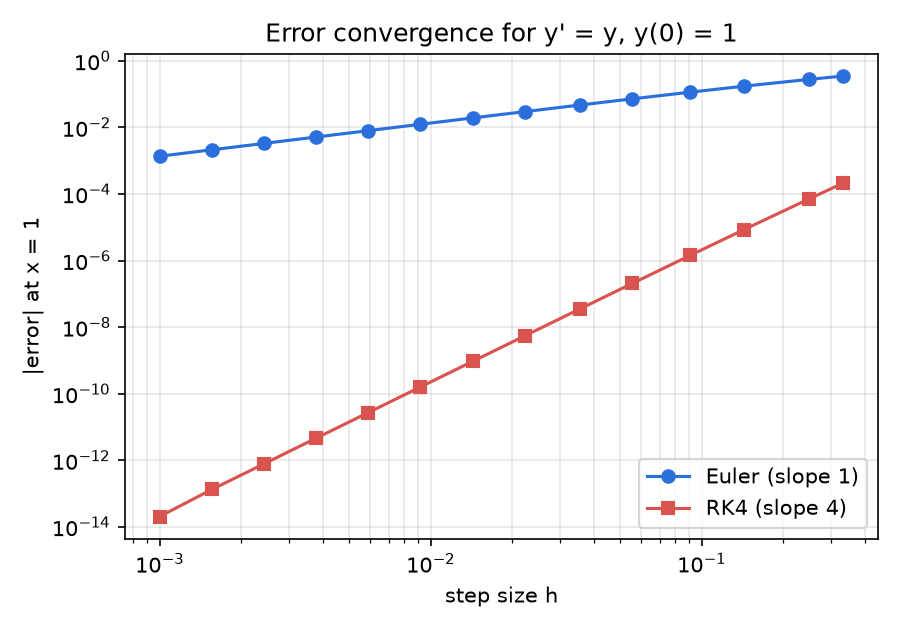
Halving the step size *h* reduces the error roughly by a factor of 2 for Euler and by a factor of 16 for RK4.
|
|
49
|
+
|
|
50
|
+
|
|
51
|
+
|
|
52
|
+
`euler_2order` updates y' first and then uses the *new* y' to update y. This keeps the energy of oscillating systems (e.g. y'' = −y) bounded, while the plain explicit Euler method lets it grow without limit.
|
|
53
|
+
|
|
54
|
+
The second-order solvers rewrite y'' = f(x, y, y') as a system of two first-order ODEs, y' = v and v' = f(x, y, v), and advance y and v together.
|
|
55
|
+
|
|
56
|
+
## Installation
|
|
57
|
+
|
|
58
|
+
```bash
|
|
59
|
+
pip install numODEsolver
|
|
60
|
+
```
|
|
61
|
+
|
|
62
|
+
Requires Python 3.8 or newer. The dependencies [NumPy](https://numpy.org), [SciPy](https://scipy.org) and [asteval](https://github.com/lmfit/asteval) are installed automatically.
|
|
63
|
+
|
|
64
|
+
## Usage
|
|
65
|
+
|
|
66
|
+
### First-order ODE
|
|
67
|
+
|
|
68
|
+
Solve y' = y with y(0) = 1 (exact solution: y = eˣ):
|
|
69
|
+
|
|
70
|
+
```python
|
|
71
|
+
import numODEsolver as ns
|
|
72
|
+
import matplotlib.pyplot as plt # optional, only for plotting
|
|
73
|
+
|
|
74
|
+
solver = ns.Solver()
|
|
75
|
+
f = solver.get_function("y") # right-hand side of y' = y
|
|
76
|
+
values = solver.rk4_1order(f, x0=0, y0=1, n=10000, bound=10)
|
|
77
|
+
|
|
78
|
+
print(solver.get_value(values, val=10, dec=5)) # y(10) ≈ e^10 = 22026.46579
|
|
79
|
+
|
|
80
|
+
plt.plot(values[:, 0], values[:, 1])
|
|
81
|
+
plt.show()
|
|
82
|
+
```
|
|
83
|
+
|
|
84
|
+
### Second-order ODE
|
|
85
|
+
|
|
86
|
+
Solve y'' = y' + y with y(0) = 1 and y'(0) = 1:
|
|
87
|
+
|
|
88
|
+
```python
|
|
89
|
+
import numODEsolver as ns
|
|
90
|
+
|
|
91
|
+
solver = ns.Solver()
|
|
92
|
+
f = solver.get_function("y'+y") # right-hand side of y'' = y' + y; use y' for the first derivative
|
|
93
|
+
values = solver.rk4_2order(f, x0=0, y0=1, dy0=1, n=10000, bound=5)
|
|
94
|
+
|
|
95
|
+
print(solver.get_value(values, val=3, dec=2)) # y(3) ≈ 92.86
|
|
96
|
+
```
|
|
97
|
+
|
|
98
|
+
`euler_2order` takes the same arguments.
|
|
99
|
+
|
|
100
|
+
### Parameters
|
|
101
|
+
|
|
102
|
+
| Parameter | Meaning |
|
|
103
|
+
| :--- | :--- |
|
|
104
|
+
| `x0`, `y0` | Initial point and initial value |
|
|
105
|
+
| `dy0` | Initial value of y' (second-order solvers only) |
|
|
106
|
+
| `n` | Number of steps (step size h = (bound − x0) / n) |
|
|
107
|
+
| `bound` | End of the integration interval, must be greater than `x0` |
|
|
108
|
+
| `val`, `dec` | x-value to evaluate and number of decimal places (`get_value`) |
|
|
109
|
+
|
|
110
|
+
### Return value
|
|
111
|
+
|
|
112
|
+
Every solver returns a NumPy array with one row per step:
|
|
113
|
+
|
|
114
|
+
- first-order solvers: columns `[x, y]`
|
|
115
|
+
- second-order solvers: columns `[x, y, y']`
|
|
116
|
+
|
|
117
|
+
`get_value` interpolates y between the steps with a cubic spline. `val` must lie between `x0` and `bound`.
|
|
118
|
+
|
|
119
|
+
## How Functions Are Parsed
|
|
120
|
+
|
|
121
|
+
`get_function` turns a string such as `"y'+y"` into a callable function:
|
|
122
|
+
|
|
123
|
+
1. The string is converted to lower case and every `y'` is replaced by a variable `dy`.
|
|
124
|
+
2. The expression is evaluated with [asteval](https://github.com/lmfit/asteval) as `lambda x, y, dy=0: <expression>`.
|
|
125
|
+
3. If the expression contains `y'`, the function is marked as second-order.
|
|
126
|
+
|
|
127
|
+
Allowed are the variables `x`, `y` and `y'`, normal Python operators (`+ - * / **`) and the NumPy math functions and constants without a prefix, e.g. `sin`, `cos`, `exp`, `log`, `sqrt`, `abs`, `pi`:
|
|
128
|
+
|
|
129
|
+
```python
|
|
130
|
+
solver.get_function("sin(x) - y**2")
|
|
131
|
+
solver.get_function("-0.5*y' - 4*y")
|
|
132
|
+
```
|
|
133
|
+
|
|
134
|
+
asteval does not allow imports or access to Python internals (like `__import__`), and numODEsolver also removes asteval's `open()`, so expressions cannot read files. This makes it much safer than Python's `eval`, but it is not a complete sandbox, so do not pass untrusted input.
|
|
135
|
+
|
|
136
|
+
An expression that cannot be parsed raises a `ValueError`. Passing a function with `y'` to a first-order solver also raises a `ValueError`.
|
|
137
|
+
|
|
138
|
+
## Known Limitations
|
|
139
|
+
|
|
140
|
+
- Fixed step size only (no adaptive step-size control)
|
|
141
|
+
- Explicit methods: stiff ODEs may require very small step sizes
|
|
142
|
+
- Integration only forwards (`bound` must be greater than `x0`)
|
|
143
|
+
- Only single equations, no systems of several ODEs and no third or higher order
|
|
144
|
+
- `get_value` needs at least 4 points (`n >= 3`) for the cubic interpolation
|
|
145
|
+
- Functions are evaluated through asteval, which is slower than plain Python; very large `n` can take a while
|
|
146
|
+
## Contributing
|
|
147
|
+
|
|
148
|
+
Bug reports and suggestions are welcome. Please open an [issue](https://github.com/lukasnf/Numerical-ODE-Solver/issues).
|
|
149
|
+
|
|
150
|
+
## Author
|
|
151
|
+
|
|
152
|
+
Lukas Filipon, B.Sc. Physics student at KIT
|
|
@@ -0,0 +1,122 @@
|
|
|
1
|
+
# numODEsolver
|
|
2
|
+
|
|
3
|
+
|
|
4
|
+

|
|
5
|
+

|
|
6
|
+
|
|
7
|
+
A lightweight Python package for solving first- and second-order ordinary differential equations (ODEs) numerically, using Euler-type methods or the classical fourth-order Runge–Kutta method (RK4).
|
|
8
|
+
|
|
9
|
+
## Methods
|
|
10
|
+
|
|
11
|
+
| Solver | ODE | Method | Global error |
|
|
12
|
+
| :--- | :--- | :--- | :--- |
|
|
13
|
+
| `euler_1order` | y' = f(x, y) | Explicit Euler | ∝ h |
|
|
14
|
+
| `rk4_1order` | y' = f(x, y) | Classical RK4 | ∝ h⁴ |
|
|
15
|
+
| `euler_2order` | y'' = f(x, y, y') | Semi-implicit Euler (Euler–Cromer) | ∝ h |
|
|
16
|
+
| `rk4_2order` | y'' = f(x, y, y') | Classical RK4 | ∝ h⁴ |
|
|
17
|
+
|
|
18
|
+
Halving the step size *h* reduces the error roughly by a factor of 2 for Euler and by a factor of 16 for RK4.
|
|
19
|
+
|
|
20
|
+

|
|
21
|
+
|
|
22
|
+
`euler_2order` updates y' first and then uses the *new* y' to update y. This keeps the energy of oscillating systems (e.g. y'' = −y) bounded, while the plain explicit Euler method lets it grow without limit.
|
|
23
|
+
|
|
24
|
+
The second-order solvers rewrite y'' = f(x, y, y') as a system of two first-order ODEs, y' = v and v' = f(x, y, v), and advance y and v together.
|
|
25
|
+
|
|
26
|
+
## Installation
|
|
27
|
+
|
|
28
|
+
```bash
|
|
29
|
+
pip install numODEsolver
|
|
30
|
+
```
|
|
31
|
+
|
|
32
|
+
Requires Python 3.8 or newer. The dependencies [NumPy](https://numpy.org), [SciPy](https://scipy.org) and [asteval](https://github.com/lmfit/asteval) are installed automatically.
|
|
33
|
+
|
|
34
|
+
## Usage
|
|
35
|
+
|
|
36
|
+
### First-order ODE
|
|
37
|
+
|
|
38
|
+
Solve y' = y with y(0) = 1 (exact solution: y = eˣ):
|
|
39
|
+
|
|
40
|
+
```python
|
|
41
|
+
import numODEsolver as ns
|
|
42
|
+
import matplotlib.pyplot as plt # optional, only for plotting
|
|
43
|
+
|
|
44
|
+
solver = ns.Solver()
|
|
45
|
+
f = solver.get_function("y") # right-hand side of y' = y
|
|
46
|
+
values = solver.rk4_1order(f, x0=0, y0=1, n=10000, bound=10)
|
|
47
|
+
|
|
48
|
+
print(solver.get_value(values, val=10, dec=5)) # y(10) ≈ e^10 = 22026.46579
|
|
49
|
+
|
|
50
|
+
plt.plot(values[:, 0], values[:, 1])
|
|
51
|
+
plt.show()
|
|
52
|
+
```
|
|
53
|
+
|
|
54
|
+
### Second-order ODE
|
|
55
|
+
|
|
56
|
+
Solve y'' = y' + y with y(0) = 1 and y'(0) = 1:
|
|
57
|
+
|
|
58
|
+
```python
|
|
59
|
+
import numODEsolver as ns
|
|
60
|
+
|
|
61
|
+
solver = ns.Solver()
|
|
62
|
+
f = solver.get_function("y'+y") # right-hand side of y'' = y' + y; use y' for the first derivative
|
|
63
|
+
values = solver.rk4_2order(f, x0=0, y0=1, dy0=1, n=10000, bound=5)
|
|
64
|
+
|
|
65
|
+
print(solver.get_value(values, val=3, dec=2)) # y(3) ≈ 92.86
|
|
66
|
+
```
|
|
67
|
+
|
|
68
|
+
`euler_2order` takes the same arguments.
|
|
69
|
+
|
|
70
|
+
### Parameters
|
|
71
|
+
|
|
72
|
+
| Parameter | Meaning |
|
|
73
|
+
| :--- | :--- |
|
|
74
|
+
| `x0`, `y0` | Initial point and initial value |
|
|
75
|
+
| `dy0` | Initial value of y' (second-order solvers only) |
|
|
76
|
+
| `n` | Number of steps (step size h = (bound − x0) / n) |
|
|
77
|
+
| `bound` | End of the integration interval, must be greater than `x0` |
|
|
78
|
+
| `val`, `dec` | x-value to evaluate and number of decimal places (`get_value`) |
|
|
79
|
+
|
|
80
|
+
### Return value
|
|
81
|
+
|
|
82
|
+
Every solver returns a NumPy array with one row per step:
|
|
83
|
+
|
|
84
|
+
- first-order solvers: columns `[x, y]`
|
|
85
|
+
- second-order solvers: columns `[x, y, y']`
|
|
86
|
+
|
|
87
|
+
`get_value` interpolates y between the steps with a cubic spline. `val` must lie between `x0` and `bound`.
|
|
88
|
+
|
|
89
|
+
## How Functions Are Parsed
|
|
90
|
+
|
|
91
|
+
`get_function` turns a string such as `"y'+y"` into a callable function:
|
|
92
|
+
|
|
93
|
+
1. The string is converted to lower case and every `y'` is replaced by a variable `dy`.
|
|
94
|
+
2. The expression is evaluated with [asteval](https://github.com/lmfit/asteval) as `lambda x, y, dy=0: <expression>`.
|
|
95
|
+
3. If the expression contains `y'`, the function is marked as second-order.
|
|
96
|
+
|
|
97
|
+
Allowed are the variables `x`, `y` and `y'`, normal Python operators (`+ - * / **`) and the NumPy math functions and constants without a prefix, e.g. `sin`, `cos`, `exp`, `log`, `sqrt`, `abs`, `pi`:
|
|
98
|
+
|
|
99
|
+
```python
|
|
100
|
+
solver.get_function("sin(x) - y**2")
|
|
101
|
+
solver.get_function("-0.5*y' - 4*y")
|
|
102
|
+
```
|
|
103
|
+
|
|
104
|
+
asteval does not allow imports or access to Python internals (like `__import__`), and numODEsolver also removes asteval's `open()`, so expressions cannot read files. This makes it much safer than Python's `eval`, but it is not a complete sandbox, so do not pass untrusted input.
|
|
105
|
+
|
|
106
|
+
An expression that cannot be parsed raises a `ValueError`. Passing a function with `y'` to a first-order solver also raises a `ValueError`.
|
|
107
|
+
|
|
108
|
+
## Known Limitations
|
|
109
|
+
|
|
110
|
+
- Fixed step size only (no adaptive step-size control)
|
|
111
|
+
- Explicit methods: stiff ODEs may require very small step sizes
|
|
112
|
+
- Integration only forwards (`bound` must be greater than `x0`)
|
|
113
|
+
- Only single equations, no systems of several ODEs and no third or higher order
|
|
114
|
+
- `get_value` needs at least 4 points (`n >= 3`) for the cubic interpolation
|
|
115
|
+
- Functions are evaluated through asteval, which is slower than plain Python; very large `n` can take a while
|
|
116
|
+
## Contributing
|
|
117
|
+
|
|
118
|
+
Bug reports and suggestions are welcome. Please open an [issue](https://github.com/lukasnf/Numerical-ODE-Solver/issues).
|
|
119
|
+
|
|
120
|
+
## Author
|
|
121
|
+
|
|
122
|
+
Lukas Filipon, B.Sc. Physics student at KIT
|
|
@@ -1,4 +1,5 @@
|
|
|
1
1
|
from scipy.interpolate import interp1d
|
|
2
|
+
import re
|
|
2
3
|
import numpy as np
|
|
3
4
|
from asteval import Interpreter
|
|
4
5
|
|
|
@@ -8,20 +9,30 @@ from asteval import Interpreter
|
|
|
8
9
|
class Solver:
|
|
9
10
|
def __init__(self):
|
|
10
11
|
self.aeval = Interpreter()
|
|
12
|
+
self.aeval.symtable.pop("open", None)
|
|
11
13
|
def get_function(self, func):
|
|
12
|
-
|
|
13
|
-
|
|
14
|
-
|
|
15
|
-
|
|
16
|
-
|
|
17
|
-
|
|
18
|
-
|
|
19
|
-
|
|
20
|
-
|
|
21
|
-
|
|
14
|
+
expr = func.lower().replace("y'", "dy")
|
|
15
|
+
f = self.aeval(f"lambda x, y, dy=0: {expr}")
|
|
16
|
+
if self.aeval.error or not callable(f):
|
|
17
|
+
msg = self.aeval.error[0].get_error() if self.aeval.error else "error"
|
|
18
|
+
self.aeval.error = []
|
|
19
|
+
raise ValueError(f"Could not parse function {func!r}: {msg}")
|
|
20
|
+
|
|
21
|
+
def wrapped(x, y, dy=0):
|
|
22
|
+
return f(x, y, dy)
|
|
23
|
+
# order 2 if the expression depends on y' (dy), otherwise order 1
|
|
24
|
+
wrapped.order = 2 if re.search(r"\bdy\b", expr) else 1
|
|
25
|
+
return wrapped
|
|
26
|
+
|
|
27
|
+
@staticmethod
|
|
28
|
+
def _check_first_order(f):
|
|
29
|
+
if getattr(f, "order", 1) == 2:
|
|
30
|
+
raise ValueError("Function contains y' – use euler_2order or rk4_2order instead.")
|
|
31
|
+
|
|
32
|
+
def euler_2order(self,f,x0,y0,dy0,n,bound): # euler cromer
|
|
22
33
|
if n <= 0:
|
|
23
34
|
raise ValueError("n must be greater than zero.")
|
|
24
|
-
elif x0
|
|
35
|
+
elif x0 >= bound:
|
|
25
36
|
raise ValueError("initial condition must be < than the input bound!")
|
|
26
37
|
vals = np.zeros((n+1,3))
|
|
27
38
|
vals[0] = [x0,y0,dy0]
|
|
@@ -31,16 +42,17 @@ class Solver:
|
|
|
31
42
|
|
|
32
43
|
dy_d = dy + h*f(x,y,dy)
|
|
33
44
|
y_d = y + h * dy_d
|
|
34
|
-
x_d =
|
|
45
|
+
x_d = x0 + (i+1)*h
|
|
35
46
|
vals[i+1] = [x_d,y_d,dy_d]
|
|
36
47
|
|
|
37
48
|
return vals
|
|
38
49
|
|
|
39
50
|
def euler_1order(self,f,x0,y0,n,bound):
|
|
51
|
+
self._check_first_order(f)
|
|
40
52
|
if n <= 0:
|
|
41
53
|
raise ValueError("n must be greater than zero.")
|
|
42
|
-
elif x0
|
|
43
|
-
raise ValueError("initial condition must be < than the
|
|
54
|
+
elif x0 >= bound:
|
|
55
|
+
raise ValueError("initial condition must be < than the input bound!")
|
|
44
56
|
vals = np.zeros((n+1, 2))
|
|
45
57
|
vals[0] = [x0,y0]
|
|
46
58
|
h = (bound-x0)/n
|
|
@@ -53,10 +65,11 @@ class Solver:
|
|
|
53
65
|
return vals
|
|
54
66
|
|
|
55
67
|
def rk4_1order(self,f,x0,y0,n,bound):
|
|
68
|
+
self._check_first_order(f)
|
|
56
69
|
if n <= 0:
|
|
57
70
|
raise ValueError("n must be greater than zero.")
|
|
58
|
-
elif x0
|
|
59
|
-
raise ValueError("initial condition must be < than the
|
|
71
|
+
elif x0 >= bound:
|
|
72
|
+
raise ValueError("initial condition must be < than the input bound!")
|
|
60
73
|
vals = np.zeros((n+1,2))
|
|
61
74
|
vals[0] = [x0,y0]
|
|
62
75
|
h = (bound-x0) / n
|
|
@@ -71,9 +84,40 @@ class Solver:
|
|
|
71
84
|
x_d = x0 + (i+1)*h
|
|
72
85
|
y_d = y + h * (k1+2*k2+2*k3+k4)/6
|
|
73
86
|
vals[i+1] = [x_d,y_d]
|
|
74
|
-
|
|
87
|
+
|
|
88
|
+
return vals
|
|
89
|
+
|
|
90
|
+
# y'' = f(x,y,y') is rewritten as a system of two first-order ODEs:
|
|
91
|
+
# y' = v, v' = f(x,y,v)
|
|
92
|
+
# and both equations are advanced together with classical RK4.
|
|
93
|
+
def rk4_2order(self,f,x0,y0,dy0,n,bound):
|
|
94
|
+
if n <= 0:
|
|
95
|
+
raise ValueError("n must be greater than zero.")
|
|
96
|
+
elif x0 >= bound:
|
|
97
|
+
raise ValueError("initial condition must be < than the input bound!")
|
|
98
|
+
vals = np.zeros((n+1,3))
|
|
99
|
+
vals[0] = [x0,y0,dy0]
|
|
100
|
+
h = (bound-x0) / n
|
|
101
|
+
for i in range(n):
|
|
102
|
+
x,y,v = vals[i]
|
|
103
|
+
|
|
104
|
+
# k = slope of y (= v), l = slope of v (= f)
|
|
105
|
+
k1 = v
|
|
106
|
+
l1 = f(x, y, v)
|
|
107
|
+
k2 = v + h/2*l1
|
|
108
|
+
l2 = f(x+h/2, y+h/2*k1, v+h/2*l1)
|
|
109
|
+
k3 = v + h/2*l2
|
|
110
|
+
l3 = f(x+h/2, y+h/2*k2, v+h/2*l2)
|
|
111
|
+
k4 = v + h*l3
|
|
112
|
+
l4 = f(x+h, y+h*k3, v+h*l3)
|
|
113
|
+
|
|
114
|
+
x_d = x0 + (i+1)*h
|
|
115
|
+
y_d = y + h * (k1+2*k2+2*k3+k4)/6
|
|
116
|
+
v_d = v + h * (l1+2*l2+2*l3+l4)/6
|
|
117
|
+
vals[i+1] = [x_d,y_d,v_d]
|
|
118
|
+
|
|
75
119
|
return vals
|
|
76
|
-
|
|
120
|
+
|
|
77
121
|
# You can adjust the decimal places, note that rk4 is more accurate
|
|
78
122
|
def get_value(self,data,val,dec):
|
|
79
123
|
x_vals = data[:,0]
|
|
@@ -0,0 +1,152 @@
|
|
|
1
|
+
Metadata-Version: 2.4
|
|
2
|
+
Name: numODEsolver
|
|
3
|
+
Version: 3.1
|
|
4
|
+
Summary: Tool that solves ODE's numerically. Written in Python.
|
|
5
|
+
Home-page: https://github.com/lukasnf/Numerical-ODE-Solver
|
|
6
|
+
License: MIT
|
|
7
|
+
Classifier: Programming Language :: Python :: 3
|
|
8
|
+
Classifier: Programming Language :: Python :: 3.8
|
|
9
|
+
Classifier: Programming Language :: Python :: 3.9
|
|
10
|
+
Classifier: Programming Language :: Python :: 3.10
|
|
11
|
+
Classifier: Programming Language :: Python :: 3.11
|
|
12
|
+
Classifier: Programming Language :: Python :: 3.12
|
|
13
|
+
Classifier: Programming Language :: Python :: 3.13
|
|
14
|
+
Classifier: Operating System :: OS Independent
|
|
15
|
+
Requires-Python: >=3.8
|
|
16
|
+
Description-Content-Type: text/markdown
|
|
17
|
+
License-File: LICENSE
|
|
18
|
+
Requires-Dist: numpy
|
|
19
|
+
Requires-Dist: asteval
|
|
20
|
+
Requires-Dist: scipy
|
|
21
|
+
Dynamic: classifier
|
|
22
|
+
Dynamic: description
|
|
23
|
+
Dynamic: description-content-type
|
|
24
|
+
Dynamic: home-page
|
|
25
|
+
Dynamic: license
|
|
26
|
+
Dynamic: license-file
|
|
27
|
+
Dynamic: requires-dist
|
|
28
|
+
Dynamic: requires-python
|
|
29
|
+
Dynamic: summary
|
|
30
|
+
|
|
31
|
+
# numODEsolver
|
|
32
|
+
|
|
33
|
+
|
|
34
|
+

|
|
35
|
+

|
|
36
|
+
|
|
37
|
+
A lightweight Python package for solving first- and second-order ordinary differential equations (ODEs) numerically, using Euler-type methods or the classical fourth-order Runge–Kutta method (RK4).
|
|
38
|
+
|
|
39
|
+
## Methods
|
|
40
|
+
|
|
41
|
+
| Solver | ODE | Method | Global error |
|
|
42
|
+
| :--- | :--- | :--- | :--- |
|
|
43
|
+
| `euler_1order` | y' = f(x, y) | Explicit Euler | ∝ h |
|
|
44
|
+
| `rk4_1order` | y' = f(x, y) | Classical RK4 | ∝ h⁴ |
|
|
45
|
+
| `euler_2order` | y'' = f(x, y, y') | Semi-implicit Euler (Euler–Cromer) | ∝ h |
|
|
46
|
+
| `rk4_2order` | y'' = f(x, y, y') | Classical RK4 | ∝ h⁴ |
|
|
47
|
+
|
|
48
|
+
Halving the step size *h* reduces the error roughly by a factor of 2 for Euler and by a factor of 16 for RK4.
|
|
49
|
+
|
|
50
|
+

|
|
51
|
+
|
|
52
|
+
`euler_2order` updates y' first and then uses the *new* y' to update y. This keeps the energy of oscillating systems (e.g. y'' = −y) bounded, while the plain explicit Euler method lets it grow without limit.
|
|
53
|
+
|
|
54
|
+
The second-order solvers rewrite y'' = f(x, y, y') as a system of two first-order ODEs, y' = v and v' = f(x, y, v), and advance y and v together.
|
|
55
|
+
|
|
56
|
+
## Installation
|
|
57
|
+
|
|
58
|
+
```bash
|
|
59
|
+
pip install numODEsolver
|
|
60
|
+
```
|
|
61
|
+
|
|
62
|
+
Requires Python 3.8 or newer. The dependencies [NumPy](https://numpy.org), [SciPy](https://scipy.org) and [asteval](https://github.com/lmfit/asteval) are installed automatically.
|
|
63
|
+
|
|
64
|
+
## Usage
|
|
65
|
+
|
|
66
|
+
### First-order ODE
|
|
67
|
+
|
|
68
|
+
Solve y' = y with y(0) = 1 (exact solution: y = eˣ):
|
|
69
|
+
|
|
70
|
+
```python
|
|
71
|
+
import numODEsolver as ns
|
|
72
|
+
import matplotlib.pyplot as plt # optional, only for plotting
|
|
73
|
+
|
|
74
|
+
solver = ns.Solver()
|
|
75
|
+
f = solver.get_function("y") # right-hand side of y' = y
|
|
76
|
+
values = solver.rk4_1order(f, x0=0, y0=1, n=10000, bound=10)
|
|
77
|
+
|
|
78
|
+
print(solver.get_value(values, val=10, dec=5)) # y(10) ≈ e^10 = 22026.46579
|
|
79
|
+
|
|
80
|
+
plt.plot(values[:, 0], values[:, 1])
|
|
81
|
+
plt.show()
|
|
82
|
+
```
|
|
83
|
+
|
|
84
|
+
### Second-order ODE
|
|
85
|
+
|
|
86
|
+
Solve y'' = y' + y with y(0) = 1 and y'(0) = 1:
|
|
87
|
+
|
|
88
|
+
```python
|
|
89
|
+
import numODEsolver as ns
|
|
90
|
+
|
|
91
|
+
solver = ns.Solver()
|
|
92
|
+
f = solver.get_function("y'+y") # right-hand side of y'' = y' + y; use y' for the first derivative
|
|
93
|
+
values = solver.rk4_2order(f, x0=0, y0=1, dy0=1, n=10000, bound=5)
|
|
94
|
+
|
|
95
|
+
print(solver.get_value(values, val=3, dec=2)) # y(3) ≈ 92.86
|
|
96
|
+
```
|
|
97
|
+
|
|
98
|
+
`euler_2order` takes the same arguments.
|
|
99
|
+
|
|
100
|
+
### Parameters
|
|
101
|
+
|
|
102
|
+
| Parameter | Meaning |
|
|
103
|
+
| :--- | :--- |
|
|
104
|
+
| `x0`, `y0` | Initial point and initial value |
|
|
105
|
+
| `dy0` | Initial value of y' (second-order solvers only) |
|
|
106
|
+
| `n` | Number of steps (step size h = (bound − x0) / n) |
|
|
107
|
+
| `bound` | End of the integration interval, must be greater than `x0` |
|
|
108
|
+
| `val`, `dec` | x-value to evaluate and number of decimal places (`get_value`) |
|
|
109
|
+
|
|
110
|
+
### Return value
|
|
111
|
+
|
|
112
|
+
Every solver returns a NumPy array with one row per step:
|
|
113
|
+
|
|
114
|
+
- first-order solvers: columns `[x, y]`
|
|
115
|
+
- second-order solvers: columns `[x, y, y']`
|
|
116
|
+
|
|
117
|
+
`get_value` interpolates y between the steps with a cubic spline. `val` must lie between `x0` and `bound`.
|
|
118
|
+
|
|
119
|
+
## How Functions Are Parsed
|
|
120
|
+
|
|
121
|
+
`get_function` turns a string such as `"y'+y"` into a callable function:
|
|
122
|
+
|
|
123
|
+
1. The string is converted to lower case and every `y'` is replaced by a variable `dy`.
|
|
124
|
+
2. The expression is evaluated with [asteval](https://github.com/lmfit/asteval) as `lambda x, y, dy=0: <expression>`.
|
|
125
|
+
3. If the expression contains `y'`, the function is marked as second-order.
|
|
126
|
+
|
|
127
|
+
Allowed are the variables `x`, `y` and `y'`, normal Python operators (`+ - * / **`) and the NumPy math functions and constants without a prefix, e.g. `sin`, `cos`, `exp`, `log`, `sqrt`, `abs`, `pi`:
|
|
128
|
+
|
|
129
|
+
```python
|
|
130
|
+
solver.get_function("sin(x) - y**2")
|
|
131
|
+
solver.get_function("-0.5*y' - 4*y")
|
|
132
|
+
```
|
|
133
|
+
|
|
134
|
+
asteval does not allow imports or access to Python internals (like `__import__`), and numODEsolver also removes asteval's `open()`, so expressions cannot read files. This makes it much safer than Python's `eval`, but it is not a complete sandbox, so do not pass untrusted input.
|
|
135
|
+
|
|
136
|
+
An expression that cannot be parsed raises a `ValueError`. Passing a function with `y'` to a first-order solver also raises a `ValueError`.
|
|
137
|
+
|
|
138
|
+
## Known Limitations
|
|
139
|
+
|
|
140
|
+
- Fixed step size only (no adaptive step-size control)
|
|
141
|
+
- Explicit methods: stiff ODEs may require very small step sizes
|
|
142
|
+
- Integration only forwards (`bound` must be greater than `x0`)
|
|
143
|
+
- Only single equations, no systems of several ODEs and no third or higher order
|
|
144
|
+
- `get_value` needs at least 4 points (`n >= 3`) for the cubic interpolation
|
|
145
|
+
- Functions are evaluated through asteval, which is slower than plain Python; very large `n` can take a while
|
|
146
|
+
## Contributing
|
|
147
|
+
|
|
148
|
+
Bug reports and suggestions are welcome. Please open an [issue](https://github.com/lukasnf/Numerical-ODE-Solver/issues).
|
|
149
|
+
|
|
150
|
+
## Author
|
|
151
|
+
|
|
152
|
+
Lukas Filipon, B.Sc. Physics student at KIT
|
|
@@ -2,17 +2,23 @@ from setuptools import setup, find_packages
|
|
|
2
2
|
|
|
3
3
|
classifiers = [
|
|
4
4
|
"Programming Language :: Python :: 3",
|
|
5
|
-
"
|
|
5
|
+
"Programming Language :: Python :: 3.8",
|
|
6
|
+
"Programming Language :: Python :: 3.9",
|
|
7
|
+
"Programming Language :: Python :: 3.10",
|
|
8
|
+
"Programming Language :: Python :: 3.11",
|
|
9
|
+
"Programming Language :: Python :: 3.12",
|
|
10
|
+
"Programming Language :: Python :: 3.13",
|
|
6
11
|
"Operating System :: OS Independent",
|
|
7
12
|
]
|
|
8
13
|
|
|
9
14
|
setup(
|
|
10
15
|
name="numODEsolver",
|
|
11
|
-
version= "
|
|
16
|
+
version= "3.1",
|
|
12
17
|
description= "Tool that solves ODE's numerically. Written in Python.",
|
|
13
18
|
long_description=open("README.md").read(),
|
|
14
19
|
long_description_content_type="text/markdown",
|
|
15
20
|
url="https://github.com/lukasnf/Numerical-ODE-Solver",
|
|
21
|
+
license="MIT",
|
|
16
22
|
packages = ["numODEsolver"],
|
|
17
23
|
install_requires=["numpy","asteval","scipy"],
|
|
18
24
|
classifiers=classifiers,
|
numodesolver-2.0.3/PKG-INFO
DELETED
|
@@ -1,75 +0,0 @@
|
|
|
1
|
-
Metadata-Version: 2.4
|
|
2
|
-
Name: numODEsolver
|
|
3
|
-
Version: 2.0.3
|
|
4
|
-
Summary: Tool that solves ODE's numerically. Written in Python.
|
|
5
|
-
Home-page: https://github.com/lukasnf/Numerical-ODE-Solver
|
|
6
|
-
Classifier: Programming Language :: Python :: 3
|
|
7
|
-
Classifier: License :: OSI Approved :: MIT License
|
|
8
|
-
Classifier: Operating System :: OS Independent
|
|
9
|
-
Requires-Python: >=3.8
|
|
10
|
-
Description-Content-Type: text/markdown
|
|
11
|
-
License-File: LICENSE
|
|
12
|
-
Requires-Dist: numpy
|
|
13
|
-
Requires-Dist: asteval
|
|
14
|
-
Requires-Dist: scipy
|
|
15
|
-
Dynamic: classifier
|
|
16
|
-
Dynamic: description
|
|
17
|
-
Dynamic: description-content-type
|
|
18
|
-
Dynamic: home-page
|
|
19
|
-
Dynamic: license-file
|
|
20
|
-
Dynamic: requires-dist
|
|
21
|
-
Dynamic: requires-python
|
|
22
|
-
Dynamic: summary
|
|
23
|
-
|
|
24
|
-
# Numerical ODE Solver
|
|
25
|
-
|
|
26
|
-
This project is a Python implementation for solving ordinary differential equations (ODEs) numerically. The script allows users to choose between two methods: Euler's Method and Runge-Kutta 4th Order Method (RK4), providing a visual representation of the solution (optional). Note: Euler's Method is more inaccurate than RK4.
|
|
27
|
-
|
|
28
|
-
## Requirements
|
|
29
|
-
Python version >= 3.8
|
|
30
|
-
|
|
31
|
-
Ensure the following Python libraries are installed:
|
|
32
|
-
|
|
33
|
-
Install it using `pip`:
|
|
34
|
-
```bash
|
|
35
|
-
pip install numODEsolver
|
|
36
|
-
```
|
|
37
|
-
## Example
|
|
38
|
-
```bash
|
|
39
|
-
import numODEsolver as ns
|
|
40
|
-
import matplotlib.pyplot as plt #optional for plot
|
|
41
|
-
|
|
42
|
-
solver = ns.Solver()
|
|
43
|
-
f = solver.get_function("y")
|
|
44
|
-
values = solver.rk4_1order(f,x0=0,y0=1,n=10000,bound=10.1)
|
|
45
|
-
n = solver.get_value(values,val=10,dec=5)
|
|
46
|
-
print(n)
|
|
47
|
-
plt.plot(values[:,0],values[:,1])
|
|
48
|
-
plt.show()
|
|
49
|
-
```
|
|
50
|
-
```bash
|
|
51
|
-
import numODEsolver as ns
|
|
52
|
-
|
|
53
|
-
solver = ns.Solver()
|
|
54
|
-
f = solver.get_function("y'+y") #y' = for 1st derivative. The ode would be y'' = y'+y
|
|
55
|
-
values = solver.euler_2order(f,x0=0,y0=1,dy0=1,n=10000,bound=5)
|
|
56
|
-
n = solver.get_value(values,val=3,dec=2)
|
|
57
|
-
print(n)
|
|
58
|
-
```
|
|
59
|
-
|
|
60
|
-
# Version History
|
|
61
|
-
|
|
62
|
-
- 8.12.2024 - v0.1 -> only 1st order ODE's are solvable, more features coming soon
|
|
63
|
-
- 15.12.2024 - v0.2 -> removed plot function
|
|
64
|
-
- 26.1.2025 - v0.3 -> included 2nd order methods, see more on GitHub
|
|
65
|
-
- 19.03.2026 - v2.0 -> more secure function handeling, more stable numerical methods.
|
|
66
|
-
|
|
67
|
-
---
|
|
68
|
-
For more documentation take a look at the source code on my GitHub.
|
|
69
|
-
|
|
70
|
-
You can modify the script to add more methods, or change visualization settings.
|
|
71
|
-
|
|
72
|
-
Contributions and suggestions are welcome!
|
|
73
|
-
|
|
74
|
-
Lukas
|
|
75
|
-
|
numodesolver-2.0.3/README.md
DELETED
|
@@ -1,52 +0,0 @@
|
|
|
1
|
-
# Numerical ODE Solver
|
|
2
|
-
|
|
3
|
-
This project is a Python implementation for solving ordinary differential equations (ODEs) numerically. The script allows users to choose between two methods: Euler's Method and Runge-Kutta 4th Order Method (RK4), providing a visual representation of the solution (optional). Note: Euler's Method is more inaccurate than RK4.
|
|
4
|
-
|
|
5
|
-
## Requirements
|
|
6
|
-
Python version >= 3.8
|
|
7
|
-
|
|
8
|
-
Ensure the following Python libraries are installed:
|
|
9
|
-
|
|
10
|
-
Install it using `pip`:
|
|
11
|
-
```bash
|
|
12
|
-
pip install numODEsolver
|
|
13
|
-
```
|
|
14
|
-
## Example
|
|
15
|
-
```bash
|
|
16
|
-
import numODEsolver as ns
|
|
17
|
-
import matplotlib.pyplot as plt #optional for plot
|
|
18
|
-
|
|
19
|
-
solver = ns.Solver()
|
|
20
|
-
f = solver.get_function("y")
|
|
21
|
-
values = solver.rk4_1order(f,x0=0,y0=1,n=10000,bound=10.1)
|
|
22
|
-
n = solver.get_value(values,val=10,dec=5)
|
|
23
|
-
print(n)
|
|
24
|
-
plt.plot(values[:,0],values[:,1])
|
|
25
|
-
plt.show()
|
|
26
|
-
```
|
|
27
|
-
```bash
|
|
28
|
-
import numODEsolver as ns
|
|
29
|
-
|
|
30
|
-
solver = ns.Solver()
|
|
31
|
-
f = solver.get_function("y'+y") #y' = for 1st derivative. The ode would be y'' = y'+y
|
|
32
|
-
values = solver.euler_2order(f,x0=0,y0=1,dy0=1,n=10000,bound=5)
|
|
33
|
-
n = solver.get_value(values,val=3,dec=2)
|
|
34
|
-
print(n)
|
|
35
|
-
```
|
|
36
|
-
|
|
37
|
-
# Version History
|
|
38
|
-
|
|
39
|
-
- 8.12.2024 - v0.1 -> only 1st order ODE's are solvable, more features coming soon
|
|
40
|
-
- 15.12.2024 - v0.2 -> removed plot function
|
|
41
|
-
- 26.1.2025 - v0.3 -> included 2nd order methods, see more on GitHub
|
|
42
|
-
- 19.03.2026 - v2.0 -> more secure function handeling, more stable numerical methods.
|
|
43
|
-
|
|
44
|
-
---
|
|
45
|
-
For more documentation take a look at the source code on my GitHub.
|
|
46
|
-
|
|
47
|
-
You can modify the script to add more methods, or change visualization settings.
|
|
48
|
-
|
|
49
|
-
Contributions and suggestions are welcome!
|
|
50
|
-
|
|
51
|
-
Lukas
|
|
52
|
-
|
|
@@ -1,75 +0,0 @@
|
|
|
1
|
-
Metadata-Version: 2.4
|
|
2
|
-
Name: numODEsolver
|
|
3
|
-
Version: 2.0.3
|
|
4
|
-
Summary: Tool that solves ODE's numerically. Written in Python.
|
|
5
|
-
Home-page: https://github.com/lukasnf/Numerical-ODE-Solver
|
|
6
|
-
Classifier: Programming Language :: Python :: 3
|
|
7
|
-
Classifier: License :: OSI Approved :: MIT License
|
|
8
|
-
Classifier: Operating System :: OS Independent
|
|
9
|
-
Requires-Python: >=3.8
|
|
10
|
-
Description-Content-Type: text/markdown
|
|
11
|
-
License-File: LICENSE
|
|
12
|
-
Requires-Dist: numpy
|
|
13
|
-
Requires-Dist: asteval
|
|
14
|
-
Requires-Dist: scipy
|
|
15
|
-
Dynamic: classifier
|
|
16
|
-
Dynamic: description
|
|
17
|
-
Dynamic: description-content-type
|
|
18
|
-
Dynamic: home-page
|
|
19
|
-
Dynamic: license-file
|
|
20
|
-
Dynamic: requires-dist
|
|
21
|
-
Dynamic: requires-python
|
|
22
|
-
Dynamic: summary
|
|
23
|
-
|
|
24
|
-
# Numerical ODE Solver
|
|
25
|
-
|
|
26
|
-
This project is a Python implementation for solving ordinary differential equations (ODEs) numerically. The script allows users to choose between two methods: Euler's Method and Runge-Kutta 4th Order Method (RK4), providing a visual representation of the solution (optional). Note: Euler's Method is more inaccurate than RK4.
|
|
27
|
-
|
|
28
|
-
## Requirements
|
|
29
|
-
Python version >= 3.8
|
|
30
|
-
|
|
31
|
-
Ensure the following Python libraries are installed:
|
|
32
|
-
|
|
33
|
-
Install it using `pip`:
|
|
34
|
-
```bash
|
|
35
|
-
pip install numODEsolver
|
|
36
|
-
```
|
|
37
|
-
## Example
|
|
38
|
-
```bash
|
|
39
|
-
import numODEsolver as ns
|
|
40
|
-
import matplotlib.pyplot as plt #optional for plot
|
|
41
|
-
|
|
42
|
-
solver = ns.Solver()
|
|
43
|
-
f = solver.get_function("y")
|
|
44
|
-
values = solver.rk4_1order(f,x0=0,y0=1,n=10000,bound=10.1)
|
|
45
|
-
n = solver.get_value(values,val=10,dec=5)
|
|
46
|
-
print(n)
|
|
47
|
-
plt.plot(values[:,0],values[:,1])
|
|
48
|
-
plt.show()
|
|
49
|
-
```
|
|
50
|
-
```bash
|
|
51
|
-
import numODEsolver as ns
|
|
52
|
-
|
|
53
|
-
solver = ns.Solver()
|
|
54
|
-
f = solver.get_function("y'+y") #y' = for 1st derivative. The ode would be y'' = y'+y
|
|
55
|
-
values = solver.euler_2order(f,x0=0,y0=1,dy0=1,n=10000,bound=5)
|
|
56
|
-
n = solver.get_value(values,val=3,dec=2)
|
|
57
|
-
print(n)
|
|
58
|
-
```
|
|
59
|
-
|
|
60
|
-
# Version History
|
|
61
|
-
|
|
62
|
-
- 8.12.2024 - v0.1 -> only 1st order ODE's are solvable, more features coming soon
|
|
63
|
-
- 15.12.2024 - v0.2 -> removed plot function
|
|
64
|
-
- 26.1.2025 - v0.3 -> included 2nd order methods, see more on GitHub
|
|
65
|
-
- 19.03.2026 - v2.0 -> more secure function handeling, more stable numerical methods.
|
|
66
|
-
|
|
67
|
-
---
|
|
68
|
-
For more documentation take a look at the source code on my GitHub.
|
|
69
|
-
|
|
70
|
-
You can modify the script to add more methods, or change visualization settings.
|
|
71
|
-
|
|
72
|
-
Contributions and suggestions are welcome!
|
|
73
|
-
|
|
74
|
-
Lukas
|
|
75
|
-
|
|
File without changes
|
|
File without changes
|
|
File without changes
|
|
File without changes
|
|
File without changes
|
|
File without changes
|
|
File without changes
|