neuralplex 0.3.0__tar.gz → 0.3.2__tar.gz
This diff represents the content of publicly available package versions that have been released to one of the supported registries. The information contained in this diff is provided for informational purposes only and reflects changes between package versions as they appear in their respective public registries.
- neuralplex-0.3.2/PKG-INFO +212 -0
- neuralplex-0.3.2/README.md +198 -0
- neuralplex-0.3.2/docs/README.md +34 -0
- {neuralplex-0.3.0 → neuralplex-0.3.2}/docs/generate_images.py +1 -1
- neuralplex-0.3.2/examples/the_digits_experiment/README.md +14 -0
- {neuralplex-0.3.0 → neuralplex-0.3.2}/examples/the_digits_experiment/main.ipynb +4 -17
- neuralplex-0.3.2/examples/the_nibble_challenge/README.md +14 -0
- {neuralplex-0.3.0 → neuralplex-0.3.2}/examples/the_nibble_challenge/main.ipynb +4 -20
- {neuralplex-0.3.0 → neuralplex-0.3.2}/examples/the_nibble_challenge/visualizations.py +1 -1
- {neuralplex-0.3.0 → neuralplex-0.3.2}/pyproject.toml +1 -1
- neuralplex-0.3.2/src/neuralplex/__about__.py +1 -0
- {neuralplex-0.3.0 → neuralplex-0.3.2}/src/neuralplex/layer.py +3 -2
- {neuralplex-0.3.0 → neuralplex-0.3.2}/src/neuralplex/network.py +3 -2
- {neuralplex-0.3.0 → neuralplex-0.3.2}/src/neuralplex/neuron.py +3 -3
- {neuralplex-0.3.0 → neuralplex-0.3.2}/tests/test.py +16 -0
- neuralplex-0.3.0/PKG-INFO +0 -254
- neuralplex-0.3.0/README.md +0 -240
- neuralplex-0.3.0/docs/README.md +0 -49
- neuralplex-0.3.0/examples/the_digits_experiment/README.md +0 -40
- neuralplex-0.3.0/examples/the_nibble_challenge/README.md +0 -40
- neuralplex-0.3.0/src/neuralplex/__about__.py +0 -1
- {neuralplex-0.3.0 → neuralplex-0.3.2}/.gitignore +0 -0
- {neuralplex-0.3.0 → neuralplex-0.3.2}/LICENSE +0 -0
- {neuralplex-0.3.0 → neuralplex-0.3.2}/docs/pyproject.toml +0 -0
- {neuralplex-0.3.0 → neuralplex-0.3.2}/examples/the_digits_experiment/pyproject.toml +0 -0
- {neuralplex-0.3.0 → neuralplex-0.3.2}/examples/the_digits_experiment/visualizations.py +0 -0
- {neuralplex-0.3.0 → neuralplex-0.3.2}/examples/the_nibble_challenge/pyproject.toml +0 -0
- {neuralplex-0.3.0 → neuralplex-0.3.2}/images/digits_confusion_matrix.png +0 -0
- {neuralplex-0.3.0 → neuralplex-0.3.2}/images/digits_predictions.png +0 -0
- {neuralplex-0.3.0 → neuralplex-0.3.2}/images/nibble_multiweight.png +0 -0
- {neuralplex-0.3.0 → neuralplex-0.3.2}/src/neuralplex/__init__.py +0 -0
- {neuralplex-0.3.0 → neuralplex-0.3.2}/tests/__init__.py +0 -0
|
@@ -0,0 +1,212 @@
|
|
|
1
|
+
Metadata-Version: 2.5
|
|
2
|
+
Name: neuralplex
|
|
3
|
+
Version: 0.3.2
|
|
4
|
+
Summary: A neural network implementation built as an explicit graph of neurons and weighted connections.
|
|
5
|
+
Project-URL: Homepage, https://github.com/adamjpatterson/neuralplex
|
|
6
|
+
Project-URL: Issues, https://github.com/adamjpatterson/neuralplex/issues
|
|
7
|
+
Author-email: FAR Analytics & Research <adpatter2000@gmail.com>
|
|
8
|
+
License-File: LICENSE
|
|
9
|
+
Classifier: License :: OSI Approved :: MIT License
|
|
10
|
+
Classifier: Operating System :: OS Independent
|
|
11
|
+
Classifier: Programming Language :: Python :: 3
|
|
12
|
+
Requires-Python: >=3.11
|
|
13
|
+
Description-Content-Type: text/markdown
|
|
14
|
+
|
|
15
|
+
# Neural-pleX
|
|
16
|
+
|
|
17
|
+
[](https://pypi.org/project/neuralplex/) [](https://pypi.org/project/neuralplex/) [](https://github.com/adamjpatterson/neuralplex/blob/main/LICENSE)
|
|
18
|
+
|
|
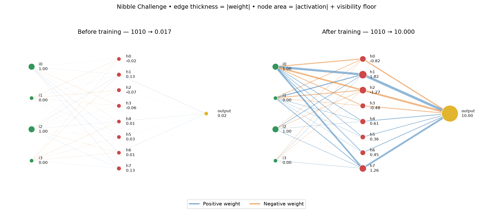
19
|
+
A neural network implementation built as an explicit graph of neurons and weighted connections.
|
|
20
|
+
|
|
21
|
+
## Introduction
|
|
22
|
+
|
|
23
|
+
**Neural-pleX** represents individual neurons and their connections explicitly, with manual backpropagation. The Neural-pleX API consists of Network, Layer, and Neuron constructors. The networks can be easily [visualized](#visualizations-of-the-network-before-and-after-training) using a visualization library.
|
|
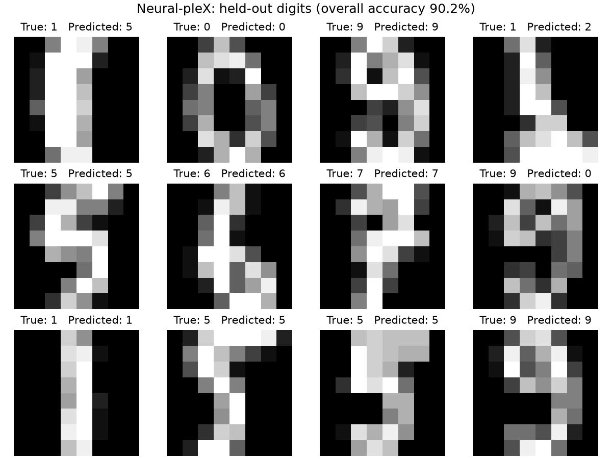
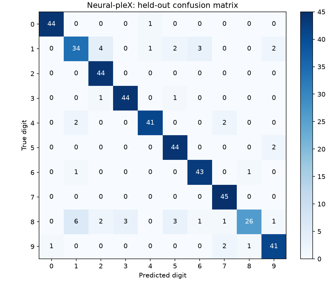
24
|
+
|
|
25
|
+
## Table of contents
|
|
26
|
+
|
|
27
|
+
- [Installation](#installation)
|
|
28
|
+
- [How it works](#how-it-works)
|
|
29
|
+
- [Examples](#examples)
|
|
30
|
+
- [The nibble challenge](#the-nibble-challenge)
|
|
31
|
+
- [The digits experiment](#the-digits-experiment)
|
|
32
|
+
- [Tests](#tests)
|
|
33
|
+
- [Documentation maintenance](#documentation-maintenance)
|
|
34
|
+
|
|
35
|
+
## Installation
|
|
36
|
+
|
|
37
|
+
To use the published package:
|
|
38
|
+
|
|
39
|
+
```bash
|
|
40
|
+
python -m pip install neuralplex
|
|
41
|
+
```
|
|
42
|
+
|
|
43
|
+
## How it works
|
|
44
|
+
|
|
45
|
+
This implementation demonstrates each component of the API. A 3 layer neural network is constructed that has a 4 neuron input Layer and a 1 neuron output layer. The hidden layer has 8 neurons.
|
|
46
|
+
|
|
47
|
+
### Implement a 3 layer neural network
|
|
48
|
+
|
|
49
|
+
#### Import the Network, Layer, and Neuron classes.
|
|
50
|
+
|
|
51
|
+
```python
|
|
52
|
+
from neuralplex import Network, Layer, Neuron
|
|
53
|
+
```
|
|
54
|
+
|
|
55
|
+
#### Set a step.
|
|
56
|
+
|
|
57
|
+
`step` is the learning rate: it controls the size of weight and bias updates. Each update subtracts `step` times the corresponding gradient. `Layer(step=...)` supplies an initial default only to neurons whose `step` is `None`. Changing `layer.step` later does not change the neurons; update each `neuron.step` directly to change its learning rate.
|
|
58
|
+
|
|
59
|
+
```python
|
|
60
|
+
STEP = 0.01
|
|
61
|
+
```
|
|
62
|
+
|
|
63
|
+
#### Construct a neural network by specifying the Neurons for each Layer and adding the Layers to a Network.
|
|
64
|
+
|
|
65
|
+
```python
|
|
66
|
+
l1 = Layer(neurons=[Neuron() for i in range(0, 4)], step=STEP)
|
|
67
|
+
l2 = Layer(neurons=[Neuron() for i in range(0, 8)], step=STEP)
|
|
68
|
+
l3 = Layer(neurons=[Neuron()], step=STEP)
|
|
69
|
+
n1 = Network([l1, l2, l3], seed=42)
|
|
70
|
+
```
|
|
71
|
+
|
|
72
|
+
#### With the Network defined, you can train the network.
|
|
73
|
+
|
|
74
|
+
Here the network is trained to recognize the nibble 1111 as the decimal number 15.
|
|
75
|
+
|
|
76
|
+
```python
|
|
77
|
+
n1.train([1,1,1,1], [15])
|
|
78
|
+
```
|
|
79
|
+
|
|
80
|
+
You can generate and print a prediction using the `predict` method. Because the network underwent just one iteration of training, the estimate will likely be inaccurate. The accuracy of the prediction can be improved by iteratively training the network. Please see [the nibble challenge](#the-nibble-challenge) for an example of how to iteratively train the network.
|
|
81
|
+
|
|
82
|
+
```python
|
|
83
|
+
prediction = n1.predict([1,1,1,1])
|
|
84
|
+
print(prediction)
|
|
85
|
+
```
|
|
86
|
+
|
|
87
|
+
### How a neuron learns
|
|
88
|
+
|
|
89
|
+
Each computational neuron calculates `activation(sum(source.value * weight) + bias)`. Inputs hold raw values. `Neuron()` uses linear activation; `Neuron(activation="tanh")` is available for hidden layers.
|
|
90
|
+
|
|
91
|
+
`Network.train` minimizes half the sum of squared output errors. It runs the forward pass, accumulates gradients backward through every connection, and only then updates weights and biases. `delta` is the derivative of the loss with respect to the neuron's weighted sum plus bias, before activation. A weight's gradient is `delta * source.value`; the bias gradient is `delta`. The code uses explicit loops, not automatic differentiation. Every non-input neuron needs a finite, positive `step` for training.
|
|
92
|
+
|
|
93
|
+
`Neuron(bias=...)` sets the bias. Each incoming connection has its own weight, stored in the receiver neuron's `weights[source]`. `Network(..., seed=42)` initializes weights reproducibly in [-0.1, 0.1]. Connections added later accept an explicit `weight`; repeated connection calls preserve existing weights.
|
|
94
|
+
|
|
95
|
+
### Explore a trained network
|
|
96
|
+
|
|
97
|
+
After training, remove a connection and compare predictions to see how it affects the network. This experiment is called an ablation.
|
|
98
|
+
|
|
99
|
+
Using your trained network as `n1`:
|
|
100
|
+
|
|
101
|
+
```python
|
|
102
|
+
inputs = [1, 0, 1, 0]
|
|
103
|
+
source = n1.layers[1].neurons[0]
|
|
104
|
+
receiver = n1.output_layer.neurons[0]
|
|
105
|
+
weight = receiver.weights[source]
|
|
106
|
+
before = n1.predict(inputs)
|
|
107
|
+
|
|
108
|
+
source.disconnectRHS(receiver)
|
|
109
|
+
after = n1.predict(inputs)
|
|
110
|
+
print("Original prediction:", before)
|
|
111
|
+
print("Without the connection:", after)
|
|
112
|
+
|
|
113
|
+
source.connectRHS(receiver, weight=weight)
|
|
114
|
+
```
|
|
115
|
+
|
|
116
|
+
Try several inputs: a connection's effect can depend on the input. To explore a whole hidden neuron, `n1.detach(neuron)` removes it from its layer and disconnects all its incoming and outgoing edges. Save those weights before detaching if you want to restore it, then add the neuron back to its layer and reconnect its edges. Its bias, activation, and learning rate remain on the object.
|
|
117
|
+
|
|
118
|
+
You can also change an existing weight through `receiver.weights[source]`. Use the connection methods to add or remove edges so incoming weights and outgoing connections stay consistent.
|
|
119
|
+
|
|
120
|
+
## Examples
|
|
121
|
+
|
|
122
|
+
### The nibble challenge
|
|
123
|
+
|
|
124
|
+
#### Setup
|
|
125
|
+
|
|
126
|
+
Change directory into the example project from the repository root.
|
|
127
|
+
|
|
128
|
+
```
|
|
129
|
+
cd examples/the_nibble_challenge
|
|
130
|
+
```
|
|
131
|
+
|
|
132
|
+
Install the example dependencies.
|
|
133
|
+
|
|
134
|
+
```
|
|
135
|
+
pip install .
|
|
136
|
+
```
|
|
137
|
+
|
|
138
|
+
#### Explore the notebook
|
|
139
|
+
|
|
140
|
+
Open [the nibble challenge notebook](https://github.com/adamjpatterson/neuralplex/blob/main/examples/the_nibble_challenge/main.ipynb). It introduces all sixteen four-bit inputs, constructs a 4 → 8 → 1 network, compares initial and trained predictions, and lets you change an input to inspect weights and activations. With seed 42, a step of 0.01, and 10,000 training examples, the displayed R² rounds to 1.000000000.
|
|
141
|
+
|
|
142
|
+
Training and evaluation both use all sixteen nibbles.
|
|
143
|
+
|
|
144
|
+
##### Visualizations of the network before and after training
|
|
145
|
+
|
|
146
|
+
|
|
147
|
+
|
|
148
|
+
- Edge thickness is proportional to the absolute connection weight. Blue is positive; orange is negative. Zero-weight edges have zero width.
|
|
149
|
+
- Node area above a small visibility floor is proportional to absolute activation. Green nodes are inputs, red nodes are hidden, and yellow is the output.
|
|
150
|
+
- Both panels use the same input, positions, and scales. Node size represents activity, not importance, and does not encode the activation's sign.
|
|
151
|
+
|
|
152
|
+
The notebook imports `visualize_network` from [its visualization module](https://github.com/adamjpatterson/neuralplex/blob/main/examples/the_nibble_challenge/visualizations.py).
|
|
153
|
+
|
|
154
|
+
### The digits experiment
|
|
155
|
+
|
|
156
|
+
#### Setup
|
|
157
|
+
|
|
158
|
+
Change directory into the example project from the repository root.
|
|
159
|
+
|
|
160
|
+
```bash
|
|
161
|
+
cd examples/the_digits_experiment
|
|
162
|
+
```
|
|
163
|
+
|
|
164
|
+
Install the example dependencies.
|
|
165
|
+
|
|
166
|
+
```bash
|
|
167
|
+
pip install .
|
|
168
|
+
```
|
|
169
|
+
|
|
170
|
+
#### Explore the notebook
|
|
171
|
+
|
|
172
|
+
Open [the digits experiment notebook](https://github.com/adamjpatterson/neuralplex/blob/main/examples/the_digits_experiment/main.ipynb). It starts by displaying the [8×8 digits dataset](https://scikit-learn.org/stable/modules/generated/sklearn.datasets.load_digits.html), then normalizes pixels, creates a training/test split, constructs a 64 → 16 → 10 network, trains, and evaluates unseen images. You can inspect an individual prediction and its ten output scores. Scores are not probabilities.
|
|
173
|
+
|
|
174
|
+
The reproducible settings use seed 42, 1,347 training images, 450 test images, 20 epochs, and a step of 0.001. The example achieves **90.22% test accuracy**, compared with **10.22%** for always predicting the most common training digit.
|
|
175
|
+
|
|
176
|
+
The notebook imports `plot_predictions` and `plot_confusion_matrix` from [its visualization module](https://github.com/adamjpatterson/neuralplex/blob/main/examples/the_digits_experiment/visualizations.py).
|
|
177
|
+
|
|
178
|
+
#### Digits predictions and confusion matrix
|
|
179
|
+
|
|
180
|
+
The prediction figure shows the first twelve test images. The confusion matrix includes all 450 test images; rows show the true digit and columns show the predicted digit.
|
|
181
|
+
|
|
182
|
+
|
|
183
|
+
|
|
184
|
+
|
|
185
|
+
|
|
186
|
+
## Tests
|
|
187
|
+
|
|
188
|
+
The suite in `tests/test.py` checks forward calculations, manual gradients, parameter updates, detachment and reconnection, and input validation.
|
|
189
|
+
|
|
190
|
+
#### Run all tests.
|
|
191
|
+
|
|
192
|
+
```bash
|
|
193
|
+
python -m unittest -v
|
|
194
|
+
```
|
|
195
|
+
|
|
196
|
+
## Documentation maintenance
|
|
197
|
+
|
|
198
|
+
### Regenerating README figures
|
|
199
|
+
|
|
200
|
+
The [documentation-image project](https://github.com/adamjpatterson/neuralplex/blob/main/docs/README.md) has its own dependencies and fixed seed-42 scenarios. From `docs/`, after following its environment setup:
|
|
201
|
+
|
|
202
|
+
```bash
|
|
203
|
+
python generate_images.py
|
|
204
|
+
```
|
|
205
|
+
|
|
206
|
+
It writes the nibble network image, digits predictions, and confusion matrix to `images/`.
|
|
207
|
+
|
|
208
|
+
## Support
|
|
209
|
+
|
|
210
|
+
If you have a feature request or run into any issues, feel free to submit an [issue](https://github.com/adamjpatterson/neuralplex/issues). You’re also welcome to reach out to one of the authors.
|
|
211
|
+
|
|
212
|
+
- [Adam Patterson](https://github.com/adamjpatterson)
|
|
@@ -0,0 +1,198 @@
|
|
|
1
|
+
# Neural-pleX
|
|
2
|
+
|
|
3
|
+
[](https://pypi.org/project/neuralplex/) [](https://pypi.org/project/neuralplex/) [](https://github.com/adamjpatterson/neuralplex/blob/main/LICENSE)
|
|
4
|
+
|
|
5
|
+
A neural network implementation built as an explicit graph of neurons and weighted connections.
|
|
6
|
+
|
|
7
|
+
## Introduction
|
|
8
|
+
|
|
9
|
+
**Neural-pleX** represents individual neurons and their connections explicitly, with manual backpropagation. The Neural-pleX API consists of Network, Layer, and Neuron constructors. The networks can be easily [visualized](#visualizations-of-the-network-before-and-after-training) using a visualization library.
|
|
10
|
+
|
|
11
|
+
## Table of contents
|
|
12
|
+
|
|
13
|
+
- [Installation](#installation)
|
|
14
|
+
- [How it works](#how-it-works)
|
|
15
|
+
- [Examples](#examples)
|
|
16
|
+
- [The nibble challenge](#the-nibble-challenge)
|
|
17
|
+
- [The digits experiment](#the-digits-experiment)
|
|
18
|
+
- [Tests](#tests)
|
|
19
|
+
- [Documentation maintenance](#documentation-maintenance)
|
|
20
|
+
|
|
21
|
+
## Installation
|
|
22
|
+
|
|
23
|
+
To use the published package:
|
|
24
|
+
|
|
25
|
+
```bash
|
|
26
|
+
python -m pip install neuralplex
|
|
27
|
+
```
|
|
28
|
+
|
|
29
|
+
## How it works
|
|
30
|
+
|
|
31
|
+
This implementation demonstrates each component of the API. A 3 layer neural network is constructed that has a 4 neuron input Layer and a 1 neuron output layer. The hidden layer has 8 neurons.
|
|
32
|
+
|
|
33
|
+
### Implement a 3 layer neural network
|
|
34
|
+
|
|
35
|
+
#### Import the Network, Layer, and Neuron classes.
|
|
36
|
+
|
|
37
|
+
```python
|
|
38
|
+
from neuralplex import Network, Layer, Neuron
|
|
39
|
+
```
|
|
40
|
+
|
|
41
|
+
#### Set a step.
|
|
42
|
+
|
|
43
|
+
`step` is the learning rate: it controls the size of weight and bias updates. Each update subtracts `step` times the corresponding gradient. `Layer(step=...)` supplies an initial default only to neurons whose `step` is `None`. Changing `layer.step` later does not change the neurons; update each `neuron.step` directly to change its learning rate.
|
|
44
|
+
|
|
45
|
+
```python
|
|
46
|
+
STEP = 0.01
|
|
47
|
+
```
|
|
48
|
+
|
|
49
|
+
#### Construct a neural network by specifying the Neurons for each Layer and adding the Layers to a Network.
|
|
50
|
+
|
|
51
|
+
```python
|
|
52
|
+
l1 = Layer(neurons=[Neuron() for i in range(0, 4)], step=STEP)
|
|
53
|
+
l2 = Layer(neurons=[Neuron() for i in range(0, 8)], step=STEP)
|
|
54
|
+
l3 = Layer(neurons=[Neuron()], step=STEP)
|
|
55
|
+
n1 = Network([l1, l2, l3], seed=42)
|
|
56
|
+
```
|
|
57
|
+
|
|
58
|
+
#### With the Network defined, you can train the network.
|
|
59
|
+
|
|
60
|
+
Here the network is trained to recognize the nibble 1111 as the decimal number 15.
|
|
61
|
+
|
|
62
|
+
```python
|
|
63
|
+
n1.train([1,1,1,1], [15])
|
|
64
|
+
```
|
|
65
|
+
|
|
66
|
+
You can generate and print a prediction using the `predict` method. Because the network underwent just one iteration of training, the estimate will likely be inaccurate. The accuracy of the prediction can be improved by iteratively training the network. Please see [the nibble challenge](#the-nibble-challenge) for an example of how to iteratively train the network.
|
|
67
|
+
|
|
68
|
+
```python
|
|
69
|
+
prediction = n1.predict([1,1,1,1])
|
|
70
|
+
print(prediction)
|
|
71
|
+
```
|
|
72
|
+
|
|
73
|
+
### How a neuron learns
|
|
74
|
+
|
|
75
|
+
Each computational neuron calculates `activation(sum(source.value * weight) + bias)`. Inputs hold raw values. `Neuron()` uses linear activation; `Neuron(activation="tanh")` is available for hidden layers.
|
|
76
|
+
|
|
77
|
+
`Network.train` minimizes half the sum of squared output errors. It runs the forward pass, accumulates gradients backward through every connection, and only then updates weights and biases. `delta` is the derivative of the loss with respect to the neuron's weighted sum plus bias, before activation. A weight's gradient is `delta * source.value`; the bias gradient is `delta`. The code uses explicit loops, not automatic differentiation. Every non-input neuron needs a finite, positive `step` for training.
|
|
78
|
+
|
|
79
|
+
`Neuron(bias=...)` sets the bias. Each incoming connection has its own weight, stored in the receiver neuron's `weights[source]`. `Network(..., seed=42)` initializes weights reproducibly in [-0.1, 0.1]. Connections added later accept an explicit `weight`; repeated connection calls preserve existing weights.
|
|
80
|
+
|
|
81
|
+
### Explore a trained network
|
|
82
|
+
|
|
83
|
+
After training, remove a connection and compare predictions to see how it affects the network. This experiment is called an ablation.
|
|
84
|
+
|
|
85
|
+
Using your trained network as `n1`:
|
|
86
|
+
|
|
87
|
+
```python
|
|
88
|
+
inputs = [1, 0, 1, 0]
|
|
89
|
+
source = n1.layers[1].neurons[0]
|
|
90
|
+
receiver = n1.output_layer.neurons[0]
|
|
91
|
+
weight = receiver.weights[source]
|
|
92
|
+
before = n1.predict(inputs)
|
|
93
|
+
|
|
94
|
+
source.disconnectRHS(receiver)
|
|
95
|
+
after = n1.predict(inputs)
|
|
96
|
+
print("Original prediction:", before)
|
|
97
|
+
print("Without the connection:", after)
|
|
98
|
+
|
|
99
|
+
source.connectRHS(receiver, weight=weight)
|
|
100
|
+
```
|
|
101
|
+
|
|
102
|
+
Try several inputs: a connection's effect can depend on the input. To explore a whole hidden neuron, `n1.detach(neuron)` removes it from its layer and disconnects all its incoming and outgoing edges. Save those weights before detaching if you want to restore it, then add the neuron back to its layer and reconnect its edges. Its bias, activation, and learning rate remain on the object.
|
|
103
|
+
|
|
104
|
+
You can also change an existing weight through `receiver.weights[source]`. Use the connection methods to add or remove edges so incoming weights and outgoing connections stay consistent.
|
|
105
|
+
|
|
106
|
+
## Examples
|
|
107
|
+
|
|
108
|
+
### The nibble challenge
|
|
109
|
+
|
|
110
|
+
#### Setup
|
|
111
|
+
|
|
112
|
+
Change directory into the example project from the repository root.
|
|
113
|
+
|
|
114
|
+
```
|
|
115
|
+
cd examples/the_nibble_challenge
|
|
116
|
+
```
|
|
117
|
+
|
|
118
|
+
Install the example dependencies.
|
|
119
|
+
|
|
120
|
+
```
|
|
121
|
+
pip install .
|
|
122
|
+
```
|
|
123
|
+
|
|
124
|
+
#### Explore the notebook
|
|
125
|
+
|
|
126
|
+
Open [the nibble challenge notebook](https://github.com/adamjpatterson/neuralplex/blob/main/examples/the_nibble_challenge/main.ipynb). It introduces all sixteen four-bit inputs, constructs a 4 → 8 → 1 network, compares initial and trained predictions, and lets you change an input to inspect weights and activations. With seed 42, a step of 0.01, and 10,000 training examples, the displayed R² rounds to 1.000000000.
|
|
127
|
+
|
|
128
|
+
Training and evaluation both use all sixteen nibbles.
|
|
129
|
+
|
|
130
|
+
##### Visualizations of the network before and after training
|
|
131
|
+
|
|
132
|
+

|
|
133
|
+
|
|
134
|
+
- Edge thickness is proportional to the absolute connection weight. Blue is positive; orange is negative. Zero-weight edges have zero width.
|
|
135
|
+
- Node area above a small visibility floor is proportional to absolute activation. Green nodes are inputs, red nodes are hidden, and yellow is the output.
|
|
136
|
+
- Both panels use the same input, positions, and scales. Node size represents activity, not importance, and does not encode the activation's sign.
|
|
137
|
+
|
|
138
|
+
The notebook imports `visualize_network` from [its visualization module](https://github.com/adamjpatterson/neuralplex/blob/main/examples/the_nibble_challenge/visualizations.py).
|
|
139
|
+
|
|
140
|
+
### The digits experiment
|
|
141
|
+
|
|
142
|
+
#### Setup
|
|
143
|
+
|
|
144
|
+
Change directory into the example project from the repository root.
|
|
145
|
+
|
|
146
|
+
```bash
|
|
147
|
+
cd examples/the_digits_experiment
|
|
148
|
+
```
|
|
149
|
+
|
|
150
|
+
Install the example dependencies.
|
|
151
|
+
|
|
152
|
+
```bash
|
|
153
|
+
pip install .
|
|
154
|
+
```
|
|
155
|
+
|
|
156
|
+
#### Explore the notebook
|
|
157
|
+
|
|
158
|
+
Open [the digits experiment notebook](https://github.com/adamjpatterson/neuralplex/blob/main/examples/the_digits_experiment/main.ipynb). It starts by displaying the [8×8 digits dataset](https://scikit-learn.org/stable/modules/generated/sklearn.datasets.load_digits.html), then normalizes pixels, creates a training/test split, constructs a 64 → 16 → 10 network, trains, and evaluates unseen images. You can inspect an individual prediction and its ten output scores. Scores are not probabilities.
|
|
159
|
+
|
|
160
|
+
The reproducible settings use seed 42, 1,347 training images, 450 test images, 20 epochs, and a step of 0.001. The example achieves **90.22% test accuracy**, compared with **10.22%** for always predicting the most common training digit.
|
|
161
|
+
|
|
162
|
+
The notebook imports `plot_predictions` and `plot_confusion_matrix` from [its visualization module](https://github.com/adamjpatterson/neuralplex/blob/main/examples/the_digits_experiment/visualizations.py).
|
|
163
|
+
|
|
164
|
+
#### Digits predictions and confusion matrix
|
|
165
|
+
|
|
166
|
+
The prediction figure shows the first twelve test images. The confusion matrix includes all 450 test images; rows show the true digit and columns show the predicted digit.
|
|
167
|
+
|
|
168
|
+

|
|
169
|
+
|
|
170
|
+

|
|
171
|
+
|
|
172
|
+
## Tests
|
|
173
|
+
|
|
174
|
+
The suite in `tests/test.py` checks forward calculations, manual gradients, parameter updates, detachment and reconnection, and input validation.
|
|
175
|
+
|
|
176
|
+
#### Run all tests.
|
|
177
|
+
|
|
178
|
+
```bash
|
|
179
|
+
python -m unittest -v
|
|
180
|
+
```
|
|
181
|
+
|
|
182
|
+
## Documentation maintenance
|
|
183
|
+
|
|
184
|
+
### Regenerating README figures
|
|
185
|
+
|
|
186
|
+
The [documentation-image project](https://github.com/adamjpatterson/neuralplex/blob/main/docs/README.md) has its own dependencies and fixed seed-42 scenarios. From `docs/`, after following its environment setup:
|
|
187
|
+
|
|
188
|
+
```bash
|
|
189
|
+
python generate_images.py
|
|
190
|
+
```
|
|
191
|
+
|
|
192
|
+
It writes the nibble network image, digits predictions, and confusion matrix to `images/`.
|
|
193
|
+
|
|
194
|
+
## Support
|
|
195
|
+
|
|
196
|
+
If you have a feature request or run into any issues, feel free to submit an [issue](https://github.com/adamjpatterson/neuralplex/issues). You’re also welcome to reach out to one of the authors.
|
|
197
|
+
|
|
198
|
+
- [Adam Patterson](https://github.com/adamjpatterson)
|
|
@@ -0,0 +1,34 @@
|
|
|
1
|
+
# README image generation
|
|
2
|
+
|
|
3
|
+
This project generates the repository's three README illustrations.
|
|
4
|
+
|
|
5
|
+
## Setup and run
|
|
6
|
+
|
|
7
|
+
Use Python 3.11 or later. From this directory in the Neuralplex checkout:
|
|
8
|
+
|
|
9
|
+
```bash
|
|
10
|
+
python -m venv .venv
|
|
11
|
+
source .venv/bin/activate
|
|
12
|
+
python -m pip install -e .. .
|
|
13
|
+
python generate_images.py
|
|
14
|
+
```
|
|
15
|
+
|
|
16
|
+
On Windows, activate with `.venv\Scripts\activate` instead.
|
|
17
|
+
|
|
18
|
+
## Fixed scenarios
|
|
19
|
+
|
|
20
|
+
The generator uses seed **42** with these settings:
|
|
21
|
+
|
|
22
|
+
- Nibbles: a linear 4 → 8 → 1 network, step 0.01, 10,000 training examples, and input `1010` for the before/after picture. Positions and visual scales are shared between the two panels.
|
|
23
|
+
- Digits: a 64 → 16 (tanh) → 10 (linear) network, step 0.001, 20 epochs, and a stratified 75%/25% training/test split. Pixels are divided by 16. Only training images are passed to `train`.
|
|
24
|
+
- Prediction samples: the first twelve test images in split order. The confusion matrix uses all 450 test images.
|
|
25
|
+
|
|
26
|
+
The script prints the nibble R² and digits accuracy, and overwrites:
|
|
27
|
+
|
|
28
|
+
- `../images/nibble_multiweight.png`
|
|
29
|
+
- `../images/digits_predictions.png`
|
|
30
|
+
- `../images/digits_confusion_matrix.png`
|
|
31
|
+
|
|
32
|
+
Review the regenerated images and update any reported README results when changing these settings.
|
|
33
|
+
|
|
34
|
+
With these settings and seed 42, the verified run prints nibble R² `1.000000000` and digits accuracy `90.22%`.
|
|
@@ -0,0 +1,14 @@
|
|
|
1
|
+
# The digits experiment
|
|
2
|
+
|
|
3
|
+
## Setup
|
|
4
|
+
|
|
5
|
+
From the repository root, change into the example directory and install its dependencies:
|
|
6
|
+
|
|
7
|
+
```bash
|
|
8
|
+
cd examples/the_digits_experiment
|
|
9
|
+
pip install .
|
|
10
|
+
```
|
|
11
|
+
|
|
12
|
+
## Explore
|
|
13
|
+
|
|
14
|
+
Open [main.ipynb](main.ipynb) and run the cells in order.
|
|
@@ -8,7 +8,7 @@
|
|
|
8
8
|
"# The digits experiment\n",
|
|
9
9
|
"Recognize handwritten digits using the [scikit-learn 8×8 digits dataset](https://scikit-learn.org/stable/modules/generated/sklearn.datasets.load_digits.html) and Neuralplex's manual backpropagation.\n",
|
|
10
10
|
"\n",
|
|
11
|
-
"Follow the [project setup instructions](README.md), then
|
|
11
|
+
"Follow the [project setup instructions](README.md), then run the cells below.\n",
|
|
12
12
|
"\n",
|
|
13
13
|
"Run cells in order. Restart the kernel and run all cells when changing model parameters; rerunning the training cell alone continues training. The final test set is for evaluation, not choosing hyperparameters. If you want to tune, first reserve a validation subset from the training data.\n"
|
|
14
14
|
]
|
|
@@ -356,7 +356,7 @@
|
|
|
356
356
|
"metadata": {},
|
|
357
357
|
"source": [
|
|
358
358
|
"## 5. Evaluate unseen images\n",
|
|
359
|
-
"Predict the test images only after training. Compare accuracy with a baseline that always predicts the most common training digit
|
|
359
|
+
"Predict the test images only after training. Compare accuracy with a baseline that always predicts the most common training digit.\n"
|
|
360
360
|
]
|
|
361
361
|
},
|
|
362
362
|
{
|
|
@@ -419,7 +419,7 @@
|
|
|
419
419
|
"metadata": {},
|
|
420
420
|
"source": [
|
|
421
421
|
"## 6. Inspect predictions and errors\n",
|
|
422
|
-
"These are the first twelve test images in split order
|
|
422
|
+
"These are the first twelve test images in split order. The confusion matrix includes all test images. Rows are true labels and columns are predictions.\n"
|
|
423
423
|
]
|
|
424
424
|
},
|
|
425
425
|
{
|
|
@@ -474,7 +474,7 @@
|
|
|
474
474
|
"metadata": {},
|
|
475
475
|
"source": [
|
|
476
476
|
"## 7. Explore one prediction\n",
|
|
477
|
-
"Change `test_position` to inspect another held-out image and its ten scores
|
|
477
|
+
"Change `test_position` to inspect another held-out image and its ten scores.\n"
|
|
478
478
|
]
|
|
479
479
|
},
|
|
480
480
|
{
|
|
@@ -533,19 +533,6 @@
|
|
|
533
533
|
"display(inspection_figure)\n",
|
|
534
534
|
"plt.close(inspection_figure)\n"
|
|
535
535
|
]
|
|
536
|
-
},
|
|
537
|
-
{
|
|
538
|
-
"cell_type": "markdown",
|
|
539
|
-
"id": "cell-18",
|
|
540
|
-
"metadata": {},
|
|
541
|
-
"source": [
|
|
542
|
-
"## Things to try\n",
|
|
543
|
-
"- Examine the most frequent confusions and the corresponding images.\n",
|
|
544
|
-
"- Change the training budget or hidden-layer size, then restart and run all cells.\n",
|
|
545
|
-
"- Reserve a validation set before comparing hyperparameters; keep the test set for the final evaluation.\n",
|
|
546
|
-
"\n",
|
|
547
|
-
"The measured accuracy above describes this split and training configuration; it is not an estimate of the best possible performance.\n"
|
|
548
|
-
]
|
|
549
536
|
}
|
|
550
537
|
],
|
|
551
538
|
"metadata": {
|
|
@@ -0,0 +1,14 @@
|
|
|
1
|
+
# The nibble challenge
|
|
2
|
+
|
|
3
|
+
## Setup
|
|
4
|
+
|
|
5
|
+
From the repository root, change into the example directory and install its dependencies:
|
|
6
|
+
|
|
7
|
+
```bash
|
|
8
|
+
cd examples/the_nibble_challenge
|
|
9
|
+
pip install .
|
|
10
|
+
```
|
|
11
|
+
|
|
12
|
+
## Explore
|
|
13
|
+
|
|
14
|
+
Open [main.ipynb](main.ipynb) and run the cells in order.
|
|
@@ -8,7 +8,7 @@
|
|
|
8
8
|
"# The nibble challenge\n",
|
|
9
9
|
"A nibble is four binary digits. We will teach a 4 → 8 → 1 network to convert them into a decimal value, then inspect how its weights and activations change.\n",
|
|
10
10
|
"\n",
|
|
11
|
-
"
|
|
11
|
+
"Follow the [project setup instructions](README.md), then run the cells below.\n",
|
|
12
12
|
"\n",
|
|
13
13
|
"Run the cells in order. To change the seed, learning rate, or training budget, **restart the kernel and run all cells**. Re-running only training continues from the existing weights.\n"
|
|
14
14
|
]
|
|
@@ -167,7 +167,7 @@
|
|
|
167
167
|
"metadata": {},
|
|
168
168
|
"source": [
|
|
169
169
|
"## 4. Train one example at a time\n",
|
|
170
|
-
"Each `train` call performs a forward pass, calculates gradients backward, and then updates parameters. The loss is half the sum of squared output errors
|
|
170
|
+
"Each `train` call performs a forward pass, calculates gradients backward, and then updates parameters. The loss is half the sum of squared output errors.\n"
|
|
171
171
|
]
|
|
172
172
|
},
|
|
173
173
|
{
|
|
@@ -232,7 +232,7 @@
|
|
|
232
232
|
"metadata": {},
|
|
233
233
|
"source": [
|
|
234
234
|
"## 5. Evaluate all sixteen nibbles\n",
|
|
235
|
-
"Compare the predictions and mean squared error
|
|
235
|
+
"Compare the predictions and mean squared error.\n"
|
|
236
236
|
]
|
|
237
237
|
},
|
|
238
238
|
{
|
|
@@ -345,9 +345,7 @@
|
|
|
345
345
|
"metadata": {},
|
|
346
346
|
"source": [
|
|
347
347
|
"## 7. Visualize before and after\n",
|
|
348
|
-
"The helper is imported from the neighboring `visualizations.py`. Both panels use the same input, positions, and scales. Blue edges are positive; orange edges are negative. Thickness shows absolute weight. Node area above a small visibility floor shows absolute activation—not importance. Input, hidden, and output nodes are green, red, and yellow
|
|
349
|
-
"\n",
|
|
350
|
-
"The helper copies the models before calculating the displayed activations; it does not modify or train them.\n"
|
|
348
|
+
"The helper is imported from the neighboring `visualizations.py`. Both panels use the same input, positions, and scales. Blue edges are positive; orange edges are negative. Thickness shows absolute weight. Node area above a small visibility floor shows absolute activation—not importance. Input, hidden, and output nodes are green, red, and yellow."
|
|
351
349
|
]
|
|
352
350
|
},
|
|
353
351
|
{
|
|
@@ -379,20 +377,6 @@
|
|
|
379
377
|
"display(network_figure)\n",
|
|
380
378
|
"plt.close(network_figure)\n"
|
|
381
379
|
]
|
|
382
|
-
},
|
|
383
|
-
{
|
|
384
|
-
"cell_type": "markdown",
|
|
385
|
-
"id": "cell-18",
|
|
386
|
-
"metadata": {},
|
|
387
|
-
"source": [
|
|
388
|
-
"## Things to try\n",
|
|
389
|
-
"- Reduce `ITERATIONS` and inspect the imperfect predictions.\n",
|
|
390
|
-
"- Change `STEP`, then restart and run all cells to compare fairly.\n",
|
|
391
|
-
"- Change the hidden-layer size and inspect the connections.\n",
|
|
392
|
-
"- Try each input nibble and observe that weights stay fixed while activations change.\n",
|
|
393
|
-
"\n",
|
|
394
|
-
"Keep these explorations separate from the formal correctness suite.\n"
|
|
395
|
-
]
|
|
396
380
|
}
|
|
397
381
|
],
|
|
398
382
|
"metadata": {
|
|
@@ -8,7 +8,7 @@ dynamic = ["version"]
|
|
|
8
8
|
authors = [
|
|
9
9
|
{ name="FAR Analytics & Research", email="adpatter2000@gmail.com" },
|
|
10
10
|
]
|
|
11
|
-
description = "
|
|
11
|
+
description = "A neural network implementation built as an explicit graph of neurons and weighted connections."
|
|
12
12
|
readme = "README.md"
|
|
13
13
|
requires-python = ">=3.11"
|
|
14
14
|
classifiers = [
|
|
@@ -0,0 +1 @@
|
|
|
1
|
+
__version__ = "0.3.2"
|
|
@@ -1,3 +1,4 @@
|
|
|
1
|
+
from math import isfinite
|
|
1
2
|
from typing import Self
|
|
2
3
|
from random import Random
|
|
3
4
|
|
|
@@ -6,8 +7,8 @@ from neuralplex.neuron import Neuron
|
|
|
6
7
|
|
|
7
8
|
class Layer:
|
|
8
9
|
def __init__(self, neurons: list[Neuron], step: float | None = None):
|
|
9
|
-
if step is not None and step <= 0:
|
|
10
|
-
raise ValueError("step must be positive")
|
|
10
|
+
if step is not None and (not isfinite(step) or step <= 0):
|
|
11
|
+
raise ValueError("step must be finite and positive")
|
|
11
12
|
self.neurons = neurons
|
|
12
13
|
self.step = step
|
|
13
14
|
for neuron in neurons:
|
|
@@ -1,3 +1,4 @@
|
|
|
1
|
+
from math import isfinite
|
|
1
2
|
from random import Random
|
|
2
3
|
|
|
3
4
|
from neuralplex.layer import Layer
|
|
@@ -48,8 +49,8 @@ class Network:
|
|
|
48
49
|
raise ValueError("Supply one target value per output neuron")
|
|
49
50
|
for layer in self.layers[1:]:
|
|
50
51
|
for neuron in layer.neurons:
|
|
51
|
-
if neuron.step is None or neuron.step <= 0:
|
|
52
|
-
raise ValueError("Every computational neuron needs a positive step")
|
|
52
|
+
if neuron.step is None or not isfinite(neuron.step) or neuron.step <= 0:
|
|
53
|
+
raise ValueError("Every computational neuron needs a finite, positive step")
|
|
53
54
|
self.predict(X_train)
|
|
54
55
|
|
|
55
56
|
# Clear all gradients, including those accumulated at input neurons.
|
|
@@ -1,4 +1,4 @@
|
|
|
1
|
-
from math import tanh
|
|
1
|
+
from math import isfinite, tanh
|
|
2
2
|
from random import uniform
|
|
3
3
|
from typing import Self
|
|
4
4
|
|
|
@@ -10,8 +10,8 @@ class Neuron:
|
|
|
10
10
|
name=None, activation: str = "linear"):
|
|
11
11
|
if activation not in ("linear", "tanh"):
|
|
12
12
|
raise ValueError("activation must be 'linear' or 'tanh'")
|
|
13
|
-
if step is not None and step <= 0:
|
|
14
|
-
raise ValueError("step must be positive")
|
|
13
|
+
if step is not None and (not isfinite(step) or step <= 0):
|
|
14
|
+
raise ValueError("step must be finite and positive")
|
|
15
15
|
self.bias = bias
|
|
16
16
|
self.step = step
|
|
17
17
|
self.name = name
|