multimetricdiagram 0.1.0__tar.gz
This diff represents the content of publicly available package versions that have been released to one of the supported registries. The information contained in this diff is provided for informational purposes only and reflects changes between package versions as they appear in their respective public registries.
- multimetricdiagram-0.1.0/LICENSE +13 -0
- multimetricdiagram-0.1.0/MANIFEST.in +1 -0
- multimetricdiagram-0.1.0/PKG-INFO +301 -0
- multimetricdiagram-0.1.0/README.md +268 -0
- multimetricdiagram-0.1.0/pyproject.toml +56 -0
- multimetricdiagram-0.1.0/setup.cfg +4 -0
- multimetricdiagram-0.1.0/src/multimetricdiagram/__init__.py +47 -0
- multimetricdiagram-0.1.0/src/multimetricdiagram/_defaults.py +18 -0
- multimetricdiagram-0.1.0/src/multimetricdiagram/_text.py +191 -0
- multimetricdiagram-0.1.0/src/multimetricdiagram/alt/__init__.py +5 -0
- multimetricdiagram-0.1.0/src/multimetricdiagram/alt/taylor/__init__.py +61 -0
- multimetricdiagram-0.1.0/src/multimetricdiagram/alt/taylor/axes.py +549 -0
- multimetricdiagram-0.1.0/src/multimetricdiagram/alt/taylor/markerstick.py +152 -0
- multimetricdiagram-0.1.0/src/multimetricdiagram/alt/taylor/metrics.py +83 -0
- multimetricdiagram-0.1.0/src/multimetricdiagram/axes.py +702 -0
- multimetricdiagram-0.1.0/src/multimetricdiagram/labels.py +554 -0
- multimetricdiagram-0.1.0/src/multimetricdiagram/legend.py +420 -0
- multimetricdiagram-0.1.0/src/multimetricdiagram/markerstick.py +455 -0
- multimetricdiagram-0.1.0/src/multimetricdiagram/metrics.py +261 -0
- multimetricdiagram-0.1.0/src/multimetricdiagram.egg-info/PKG-INFO +301 -0
- multimetricdiagram-0.1.0/src/multimetricdiagram.egg-info/SOURCES.txt +41 -0
- multimetricdiagram-0.1.0/src/multimetricdiagram.egg-info/dependency_links.txt +1 -0
- multimetricdiagram-0.1.0/src/multimetricdiagram.egg-info/requires.txt +10 -0
- multimetricdiagram-0.1.0/src/multimetricdiagram.egg-info/top_level.txt +1 -0
- multimetricdiagram-0.1.0/tests/conftest.py +12 -0
- multimetricdiagram-0.1.0/tests/test_axes.py +194 -0
- multimetricdiagram-0.1.0/tests/test_axes_helpers.py +109 -0
- multimetricdiagram-0.1.0/tests/test_labels.py +153 -0
- multimetricdiagram-0.1.0/tests/test_labels_keep.py +168 -0
- multimetricdiagram-0.1.0/tests/test_labels_obstacles.py +127 -0
- multimetricdiagram-0.1.0/tests/test_labels_placement.py +406 -0
- multimetricdiagram-0.1.0/tests/test_legend.py +440 -0
- multimetricdiagram-0.1.0/tests/test_markerstick.py +484 -0
- multimetricdiagram-0.1.0/tests/test_metrics.py +169 -0
- multimetricdiagram-0.1.0/tests/test_metrics_period.py +120 -0
- multimetricdiagram-0.1.0/tests/test_return_artists.py +85 -0
- multimetricdiagram-0.1.0/tests/test_smoke.py +28 -0
- multimetricdiagram-0.1.0/tests/test_taylor_axes.py +285 -0
- multimetricdiagram-0.1.0/tests/test_taylor_docs.py +11 -0
- multimetricdiagram-0.1.0/tests/test_taylor_integration.py +59 -0
- multimetricdiagram-0.1.0/tests/test_taylor_markerstick.py +199 -0
- multimetricdiagram-0.1.0/tests/test_taylor_metrics.py +44 -0
- multimetricdiagram-0.1.0/tests/test_text_polar.py +162 -0
|
@@ -0,0 +1,13 @@
|
|
|
1
|
+
BSD 3-Clause License
|
|
2
|
+
|
|
3
|
+
Copyright (c) 2026, Daniel L. Codiga
|
|
4
|
+
|
|
5
|
+
Redistribution and use in source and binary forms, with or without modification, are permitted provided that the following conditions are met:
|
|
6
|
+
|
|
7
|
+
1. Redistributions of source code must retain the above copyright notice, this list of conditions and the following disclaimer.
|
|
8
|
+
|
|
9
|
+
2. Redistributions in binary form must reproduce the above copyright notice, this list of conditions and the following disclaimer in the documentation and/or other materials provided with the distribution.
|
|
10
|
+
|
|
11
|
+
3. Neither the name of the copyright holder nor the names of its contributors may be used to endorse or promote products derived from this software without specific prior written permission.
|
|
12
|
+
|
|
13
|
+
THIS SOFTWARE IS PROVIDED BY THE COPYRIGHT HOLDERS AND CONTRIBUTORS "AS IS" AND ANY EXPRESS OR IMPLIED WARRANTIES, INCLUDING, BUT NOT LIMITED TO, THE IMPLIED WARRANTIES OF MERCHANTABILITY AND FITNESS FOR A PARTICULAR PURPOSE ARE DISCLAIMED. IN NO EVENT SHALL THE COPYRIGHT HOLDER OR CONTRIBUTORS BE LIABLE FOR ANY DIRECT, INDIRECT, INCIDENTAL, SPECIAL, EXEMPLARY, OR CONSEQUENTIAL DAMAGES (INCLUDING, BUT NOT LIMITED TO, PROCUREMENT OF SUBSTITUTE GOODS OR SERVICES; LOSS OF USE, DATA, OR PROFITS; OR BUSINESS INTERRUPTION) HOWEVER CAUSED AND ON ANY THEORY OF LIABILITY, WHETHER IN CONTRACT, STRICT LIABILITY, OR TORT (INCLUDING NEGLIGENCE OR OTHERWISE) ARISING IN ANY WAY OUT OF THE USE OF THIS SOFTWARE, EVEN IF ADVISED OF THE POSSIBILITY OF SUCH DAMAGE.
|
|
@@ -0,0 +1 @@
|
|
|
1
|
+
recursive-include tests *.py
|
|
@@ -0,0 +1,301 @@
|
|
|
1
|
+
Metadata-Version: 2.4
|
|
2
|
+
Name: multimetricdiagram
|
|
3
|
+
Version: 0.1.0
|
|
4
|
+
Summary: Multimetric diagram: 5-metric (total/bias/pattern/amplitude/phase) alternative, that rewards realistic variance, to Taylor diagram
|
|
5
|
+
Author-email: "Daniel L. Codiga" <dcodiga@uri.edu>
|
|
6
|
+
License-Expression: BSD-3-Clause
|
|
7
|
+
Project-URL: Homepage, https://github.com/oceanmodeling/multimetricdiagram
|
|
8
|
+
Project-URL: Repository, https://github.com/oceanmodeling/multimetricdiagram
|
|
9
|
+
Project-URL: Issues, https://github.com/oceanmodeling/multimetricdiagram/issues
|
|
10
|
+
Keywords: model evaluation,skill assessment,Taylor diagram,oceanography,matplotlib
|
|
11
|
+
Classifier: Development Status :: 4 - Beta
|
|
12
|
+
Classifier: Programming Language :: Python :: 3
|
|
13
|
+
Classifier: Programming Language :: Python :: 3 :: Only
|
|
14
|
+
Classifier: Programming Language :: Python :: 3.11
|
|
15
|
+
Classifier: Programming Language :: Python :: 3.12
|
|
16
|
+
Classifier: Programming Language :: Python :: 3.13
|
|
17
|
+
Classifier: Programming Language :: Python :: 3.14
|
|
18
|
+
Classifier: Operating System :: OS Independent
|
|
19
|
+
Classifier: Intended Audience :: Science/Research
|
|
20
|
+
Classifier: Topic :: Scientific/Engineering :: Visualization
|
|
21
|
+
Requires-Python: >=3.11
|
|
22
|
+
Description-Content-Type: text/markdown
|
|
23
|
+
License-File: LICENSE
|
|
24
|
+
Requires-Dist: numpy>=1.26
|
|
25
|
+
Requires-Dist: matplotlib>=3.8
|
|
26
|
+
Provides-Extra: test
|
|
27
|
+
Requires-Dist: pytest; extra == "test"
|
|
28
|
+
Requires-Dist: pytest-cov; extra == "test"
|
|
29
|
+
Provides-Extra: dev
|
|
30
|
+
Requires-Dist: ruff; extra == "dev"
|
|
31
|
+
Requires-Dist: pylint; extra == "dev"
|
|
32
|
+
Dynamic: license-file
|
|
33
|
+
|
|
34
|
+
[](https://pypi.org/project/multimetricdiagram/)
|
|
35
|
+
[](https://anaconda.org/conda-forge/multimetricdiagram)
|
|
36
|
+
[](https://github.com/oceanmodeling/multimetricdiagram/actions/workflows/run_tests.yml)
|
|
37
|
+
[](https://github.com/oceanmodeling/multimetricdiagram/actions/workflows/pylint.yml)
|
|
38
|
+
[](https://codecov.io/gh/oceanmodeling/multimetricdiagram)
|
|
39
|
+
|
|
40
|
+

|
|
41
|
+
|
|
42
|
+
# multimetricdiagram
|
|
43
|
+
|
|
44
|
+
This package enables creation of multimetric diagrams. A multimetric diagram is a polar plot to visualize quantified differences/similarities of paired model and observation scalar or vector arrays (e.g., an array of scalar or vector model values and an array of associated observations; can be time series, spatial data, or any index). This includes (for each pair, through one markerstick on the plot) the total root mean square difference (RMSD) normalized by the model and observation standard deviations in quadrature (SDQ), its bias and pattern components, and the amplitude and phase contributions to the pattern component. (Amplitude and phase are used here, for convenience, in the broad sense that does not assume periodic signals: amplitude refers to the strength of variability, as measured by the standard deviation or variance, and phase refers to the degree to which model and observations vary together, as measured by the correlation coefficient.) The markerstick tip-ends are ordered by RMSD/SDQ and hence by their values of the Diagnostic Index of Agreement with Symmetry (DIAS). The multimetric diagram and DIAS are framed here in terms of model-observation pairs but they are also applicable to model-model comparisons or evaluations of paired observations collected by different measurement methods. The multimetric diagram is similar to a normalized Taylor diagram that includes bias sticks, with the main exceptions being that (1) the perfection star is co-located with the polar plot origin, and (2) it orders the model-observation comparisons, indicated by the distance between stick-ends of the markersticks and the 'perfection' star, by DIAS (not Nash-Sutcliffe efficiency, as in a Taylor diagram) and therefore rewards realistic variance (unlike the reward of NSE for damped variance).
|
|
45
|
+
|
|
46
|
+
## Installation
|
|
47
|
+
|
|
48
|
+
Requires Python 3.11 or later. Dependencies: numpy 1.26 or later, matplotlib 3.8 or later.
|
|
49
|
+
|
|
50
|
+
### PyPI
|
|
51
|
+
|
|
52
|
+
pip install multimetricdiagram
|
|
53
|
+
|
|
54
|
+
### Conda / Mamba
|
|
55
|
+
|
|
56
|
+
mamba install -c conda-forge multimetricdiagram
|
|
57
|
+
|
|
58
|
+
### From source (local, editable)
|
|
59
|
+
|
|
60
|
+
From this folder:
|
|
61
|
+
|
|
62
|
+
pip install -e .
|
|
63
|
+
|
|
64
|
+
With conda: install the dependencies from conda-forge, then the package without dependencies:
|
|
65
|
+
|
|
66
|
+
conda install -c conda-forge numpy matplotlib
|
|
67
|
+
pip install --no-deps -e .
|
|
68
|
+
|
|
69
|
+
The usage examples below assume the package is imported as:
|
|
70
|
+
|
|
71
|
+
import multimetricdiagram as mmd
|
|
72
|
+
|
|
73
|
+
## Explanation of diagram elements
|
|
74
|
+
|
|
75
|
+
|
|
76
|
+
|
|
77
|
+
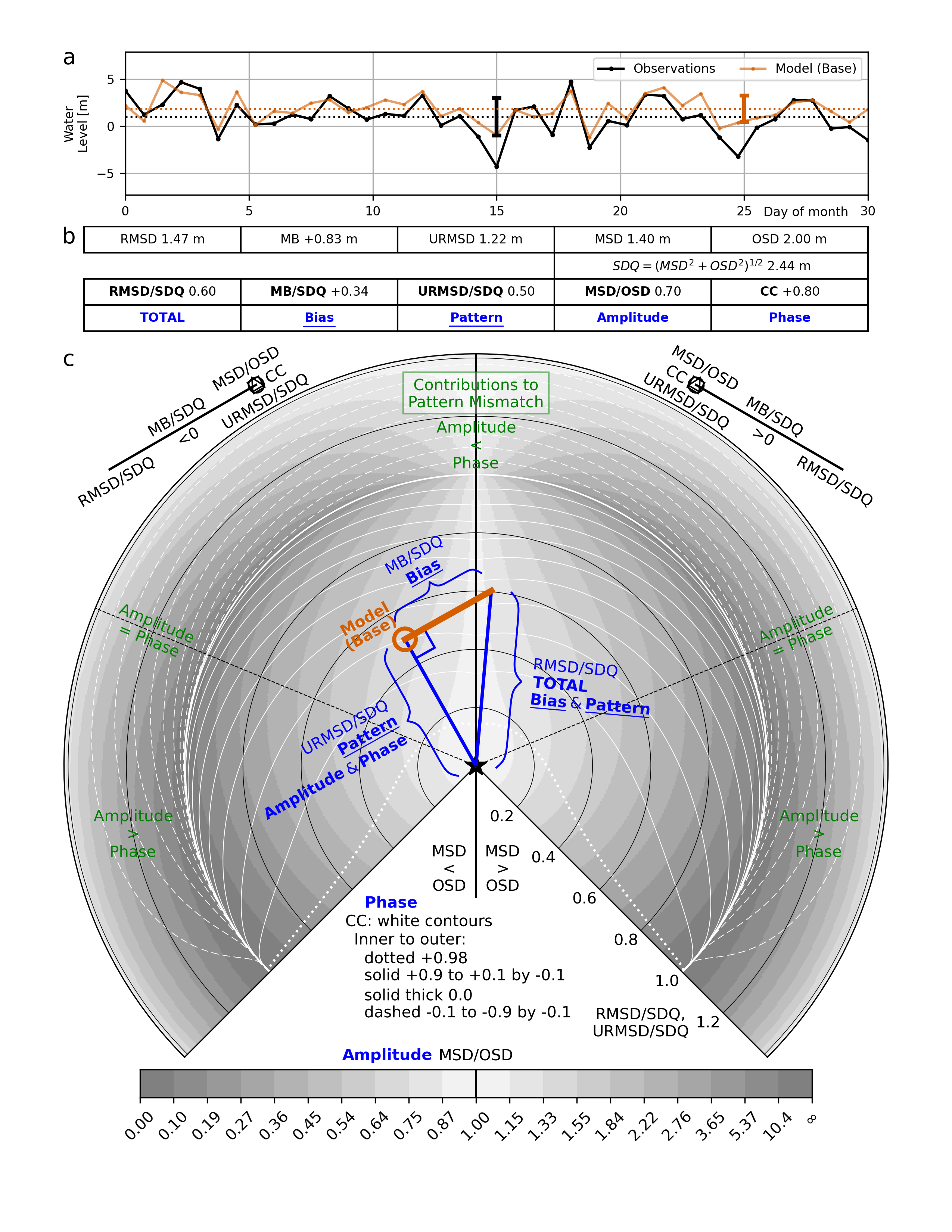
*Definitions figure: (a) an example model and observation time series, (b) the corresponding metrics, and (c) the resulting markerstick (orange); the Pythagorean triangle (blue) relating RMSD/SDQ (total), MB/SDQ (bias) and URMSD/SDQ (pattern); and green labels marking where amplitude or phase contributions to the pattern difference are dominant.*
|
|
78
|
+
|
|
79
|
+
* Each model-observation comparison is shown as a single markerstick. A markerstick is a marker symbol with a 'stick', which is a line tangential to the circular gridline through the marker location, emanating from the marker.
|
|
80
|
+
|
|
81
|
+
* Perfect model-observation agreement corresponds to a zero-length stick with marker positioned at the origin, indicated by the star.
|
|
82
|
+
|
|
83
|
+
* The distance of the tip or stick-end of the markerstick (end opposite to the marker) from the origin is an indication of the total difference metric: RMSD/SDQ, which is the Root-Mean-Square Difference RMSD normalized by SDQ, the Standard Deviations in Quadrature (Model Standard Deviation MSD, and Observation Standard Deviation OSD, in quadrature). The standard deviations are defined in the standard ways for scalars (square root of summed squared anomalies relative to mean, normalized by the number of values n) and vectors (square root of summed squared vector anomalies relative to mean, normalized by n).
|
|
84
|
+
|
|
85
|
+
* The length of the stick (distance between marker and stick-end) indicates the normalized mean bias metric MB/SDQ (Mean Bias normalized by SDQ), positive/negative for stick emanating from the marker in the clockwise/counterclockwise direction. For vectors, MB is the magnitude of the difference between the mean model vector and the mean observed vector, positive when that difference has a component along the mean observed vector and negative when it has a component opposite to it (positive for the edge case of the difference vector perpendicular to mean observation vector).
|
|
86
|
+
|
|
87
|
+
* The distance of the marker from the origin is an indication of the pattern difference metric: URMSD/SDQ (unbiased RMSD normalized by SDQ), which by definition has maximum value sqrt(2).
|
|
88
|
+
|
|
89
|
+
* The right-angle triangle geometry of (1) the hypotenuse distance from the origin to the stick-end (RMSD/SDQ), (2) the distance from the origin to the marker (URMSD/SDQ), and (3) the length of the stick (MB/SDQ) embodies the "total = bias + pattern" Pythagorean relationship (RMSD/SDQ)^2 = (URMSD/SDQ)^2 + (MB/SDQ)^2. Thus it presents the relative proportions of RMSD/SDQ, URMSD/SDQ, and MB/SDQ, and equivalently the relative proportions of the un-normalized RMSD, URMSD, and MB.
|
|
90
|
+
|
|
91
|
+
* The position of the marker relative to the grayscale shading (see grayscale bar key below bottom of polar plot) indicates MSD/OSD, the metric for the amplitude contribution to the pattern difference. The vertical axis of the plot is where MSD=OSD, perfect agreement. MSD/OSD changes with distance from there, increasing to the right and decreasing to the left, asymmetrically; the Variance Similarity VS = 2·MSD·OSD/(MSD² + OSD²) = MSD·OSD/(0.5·SDQ²) (range 0 to 1) is also 1 on the vertical axis, and decreases symmetrically with marker distance from there rightward and leftward. There is a one to one relationship between VS and MSD/OSD values: VS = 2·(MSD/OSD) / [(MSD/OSD)² + 1].
|
|
92
|
+
|
|
93
|
+
* For scalars, the Pearson correlation coefficient CC (range 1 to -1), the metric for phase agreement, is indicated by the position of the marker relative to the white contours. CC is 1 at the origin and along the radial boundaries of the polar plot at theta=-45 and -135 deg inside the unit circle, and -1 along those boundaries outside it (where theta is defined positive counter-clockwise from the rightward direction); CC is positive (dotted and solid white contours) inside the unit circle, zero at the unit circle, and negative (dashed white contours) outside the unit circle. For vectors, CC is the vector correlation coefficient based on the dot product of the vector anomalies.
|
|
94
|
+
|
|
95
|
+
* The location of the marker relative to the gray shading and the white contours for CC embodies the definitional relationship (URMSD/SDQ)^2 = 1 - VS\*CC among the pattern difference and its amplitude and phase contributions, in which there are two contributions to increasing URMSD/SDQ: (a) the extent to which VS is less than 1 (amplitude), and (b) the extent to which CC is less than 1 (phase).
|
|
96
|
+
|
|
97
|
+
* A marker located on the dotted black radial grid lines (at 67.5 degrees leftward and rightward from the vertically upward axis) indicates equal contributions to URMSD/SDQ, per (URMSD/SDQ)^2 = 1 - VS\*CC, by (a) the extent to which VS is less than 1 (amplitude), and (b) the extent to which CC is less than 1 (phase).
|
|
98
|
+
|
|
99
|
+
* A marker located outside that sector indicates the main contributor to URMSD/SDQ is the extent to which VS is less than 1 (amplitude); conversely, marker located in upper central sector of polar plot between the two dotted black radial grid lines indicates the main contributor to URMSD/SDQ is the extent to which CC is less than 1 (phase).
|
|
100
|
+
|
|
101
|
+
## Usage examples:
|
|
102
|
+
|
|
103
|
+
Save figures at dpi=300 or more for clear images (the layout does not depend on dpi; matplotlib's default is 100 dpi).
|
|
104
|
+
|
|
105
|
+
The examples use these lists, one entry per station: stnslist (station names), depth (bottom depths), TempSurfaceMod/TempSurfaceObs and TempBottomMod/TempBottomObs (temperature time series, arrays of shape (n,)), and CurrentSurfaceMod/CurrentSurfaceObs (velocity time series, arrays of shape (n, 2)). Runnable versions are in the usage_examples folder: example1.py to example6.py, with synthetic data from example_data.py. Run them from that folder, e.g. python example1.py; each saves its plot there (example1.png, ...).
|
|
106
|
+
|
|
107
|
+
Ex 1: One group of model-observation pairs; default marker style, no marker labels; legend in the legend axes above the diagram; legend by Matplotlib's built-in ax.legend(), simpler and more direct than add_labeledmarker_legend() because no marker labels are needed.
|
|
108
|
+
|
|
109
|
+
fig, ax_polar, ax_legend = mmd.make_fig_axes()
|
|
110
|
+
for mod, obs in zip(TempSurfaceMod, TempSurfaceObs):
|
|
111
|
+
ms = mmd.add_markerstick(ax_polar, mmd.calculate_metrics(mod, obs))
|
|
112
|
+
ax_legend.legend([ms.marker], ['Near-Surface Temperature'], loc='center')
|
|
113
|
+
fig.savefig('example1.png', dpi=300)
|
|
114
|
+
|
|
115
|
+
Ex 2: Same as Ex 1, but: one label per markerstick; labeledmarker legend.
|
|
116
|
+
|
|
117
|
+
fig, ax_polar, ax_legend = mmd.make_fig_axes()
|
|
118
|
+
for stn, mod, obs in zip(stnslist, TempSurfaceMod, TempSurfaceObs):
|
|
119
|
+
mmd.add_markerstick(ax_polar, mmd.calculate_metrics(mod, obs), label_info={'text': stn})
|
|
120
|
+
legend_entry = {'label': 'Near-Surface Temperature', 'label_info': {'text': 'StnID'}}
|
|
121
|
+
mmd.add_labeledmarker_legend(ax_legend, legend_entry, loc='center')
|
|
122
|
+
fig.savefig('example2.png', dpi=300)
|
|
123
|
+
|
|
124
|
+
Ex 3: Same as Ex 2, but: near-bottom temperature; two labels per markerstick; custom markerstick style; legend at lower left on polar axes.
|
|
125
|
+
|
|
126
|
+
fig, ax_polar, _ = mmd.make_fig_axes() # legend axes not used
|
|
127
|
+
style = {'marker': 's', 'color': 'b'}
|
|
128
|
+
for stn, z, mod, obs in zip(stnslist, depth, TempBottomMod, TempBottomObs):
|
|
129
|
+
labels = [{'text': stn, 'position': 'beside'}, {'text': z, 'position': 'inside'}]
|
|
130
|
+
mmd.add_markerstick(ax_polar, mmd.calculate_metrics(mod, obs),
|
|
131
|
+
markerstick_style=style, label_info=labels)
|
|
132
|
+
legend_labels = [{'text': 'StnID', 'position': 'beside'},
|
|
133
|
+
{'text': 'Depth [m]', 'position': 'inside'}]
|
|
134
|
+
legend_entry = {'label': 'Near-Bottom Temperature', 'markerstick_style': style,
|
|
135
|
+
'label_info': legend_labels}
|
|
136
|
+
# legend inside the diagram: its upper-left corner at (0.02, 0.42), in fractions of ax_polar
|
|
137
|
+
mmd.add_labeledmarker_legend(ax_polar, legend_entry,
|
|
138
|
+
loc='upper left', bbox_to_anchor=(0.02, 0.42))
|
|
139
|
+
fig.savefig('example3.png', dpi=300)
|
|
140
|
+
|
|
141
|
+
Ex 4: Groups of Ex 2 and Ex 3 superposed on one diagram; labeledmarker legend with two items (one add_labeledmarker_legend() call, 2-item list passed); legend at lower left on polar axes.
|
|
142
|
+
|
|
143
|
+
fig, ax_polar, _ = mmd.make_fig_axes() # legend axes not used
|
|
144
|
+
style = {'marker': 's', 'color': 'b'}
|
|
145
|
+
for i, stn in enumerate(stnslist):
|
|
146
|
+
surface = mmd.calculate_metrics(TempSurfaceMod[i], TempSurfaceObs[i])
|
|
147
|
+
mmd.add_markerstick(ax_polar, surface, label_info={'text': stn})
|
|
148
|
+
bottom = mmd.calculate_metrics(TempBottomMod[i], TempBottomObs[i])
|
|
149
|
+
labels = [{'text': stn, 'position': 'beside'}, {'text': depth[i], 'position': 'inside'}]
|
|
150
|
+
mmd.add_markerstick(ax_polar, bottom, markerstick_style=style, label_info=labels)
|
|
151
|
+
legend_labels = [{'text': 'StnID', 'position': 'beside'},
|
|
152
|
+
{'text': 'Depth [m]', 'position': 'inside'}]
|
|
153
|
+
mmd.add_labeledmarker_legend(ax_polar, [
|
|
154
|
+
{'label': 'Near-Surface Temperature', 'label_info': {'text': 'StnID'}},
|
|
155
|
+
{'label': 'Near-Bottom Temperature', 'markerstick_style': style, 'label_info': legend_labels},
|
|
156
|
+
], loc='upper left', bbox_to_anchor=(0.02, 0.42))
|
|
157
|
+
fig.savefig('example4.png', dpi=300)
|
|
158
|
+
|
|
159
|
+
Ex 5: Vector inputs (near-surface current); six model-observation pairs whose markersticks crowd together, labels repositioned by adjust_markerstick_labels() to avoid overlap.
|
|
160
|
+
|
|
161
|
+
fig, ax_polar, _ = mmd.make_fig_axes() # legend axes not used
|
|
162
|
+
style = {'marker': '^'}
|
|
163
|
+
results = []
|
|
164
|
+
for stn, mod, obs in zip(stnslist, CurrentSurfaceMod, CurrentSurfaceObs):
|
|
165
|
+
metrics = mmd.calculate_metrics(mod, obs)
|
|
166
|
+
results.append(mmd.add_markerstick(ax_polar, metrics, markerstick_style=style,
|
|
167
|
+
label_info={'text': stn}))
|
|
168
|
+
mmd.adjust_markerstick_labels(ax_polar, results)
|
|
169
|
+
legend_entry = {'label': 'Near-Surface Current', 'markerstick_style': style,
|
|
170
|
+
'label_info': {'text': 'StnID'}}
|
|
171
|
+
mmd.add_labeledmarker_legend(ax_polar, legend_entry,
|
|
172
|
+
loc='upper left', bbox_to_anchor=(0.02, 0.42))
|
|
173
|
+
fig.savefig('example5.png', dpi=300)
|
|
174
|
+
|
|
175
|
+
Ex 6: Same as Ex 2, but on a Taylor diagram (multimetricdiagram.alt.taylor). The metrics are passed to make_fig_axes() so it can choose one- or two-quadrant variant, and the outer radius. Two example figures: patternonly=True, bias set to zero, only markers with no bias sticks, example6_patternonly.png; then default (patternonly=False) so bias sticks are shown, example6.png. In the latter, note the stations appear in different order, by distance of stick end to star, compared to Ex 2; the ordering is by NSE here and by DIAS in Ex 2.
|
|
176
|
+
|
|
177
|
+
taylor = mmd.alt.taylor
|
|
178
|
+
for patternonly in (True, False):
|
|
179
|
+
metrics = [taylor.calculate_metrics(mod, obs, patternonly=patternonly)
|
|
180
|
+
for mod, obs in zip(TempSurfaceMod, TempSurfaceObs)]
|
|
181
|
+
fig, ax_polar, ax_legend = taylor.make_fig_axes(metrics=metrics, patternonly=patternonly)
|
|
182
|
+
for stn, m in zip(stnslist, metrics):
|
|
183
|
+
taylor.add_markerstick(ax_polar, m, label_info={'text': stn})
|
|
184
|
+
legend_entry = {'label': 'Near-Surface Temperature', 'label_info': {'text': 'StnID'}}
|
|
185
|
+
taylor.add_labeledmarker_legend(ax_legend, legend_entry, loc='center')
|
|
186
|
+
fig.savefig('example6_patternonly.png' if patternonly else 'example6.png', dpi=300)
|
|
187
|
+
|
|
188
|
+
## Purposes of functions
|
|
189
|
+
|
|
190
|
+
Main functions
|
|
191
|
+
calculate_metrics()
|
|
192
|
+
Compute metrics from model-observation pairs (scalar or vector)
|
|
193
|
+
make_fig_axes()
|
|
194
|
+
Generate figure, main polar axes, legend container axes above
|
|
195
|
+
add_markerstick()
|
|
196
|
+
Add markerstick to polar axes, metrics for a model-observation pair
|
|
197
|
+
adjust_markerstick_labels()
|
|
198
|
+
Reposition markerstick labels to minimize overlap
|
|
199
|
+
add_labeledmarker_legend()
|
|
200
|
+
Add a marker legend, optionally with text labels on markers
|
|
201
|
+
|
|
202
|
+
The text_polar() helper function (see full list of helpers below) is public on purpose, as matplotlib's ax.text() with rotation is unreliable on polar axes. The package draws its rotated text (markerstick labels and the text on and around the polar axes) with text_polar() instead. It is public so that users can add their own rotated annotations to the diagram the same way.
|
|
203
|
+
|
|
204
|
+
calculate_metrics(model, observation, period=None, ...) takes arrays of shape (n,) for scalars or (n, 2) for vectors (e.g. east and north components), of equal shape and with no NaN or inf values, and returns a dict of metrics; see its docstring for the full list and definitions. Circular scalar variables such as a phase angle can be handled (for any input range e.g. -180 to 180 deg, 0 to 360 deg, 1 to 12 months) by passing the period (period=360 for degrees, 2*np.pi for radians, 24 for hour of day), observations are taken as angles from their circular mean and the model-observation differences use within-cycle distances.
|
|
205
|
+
|
|
206
|
+
make_fig_axes(**overrides) accepts settings that replace its defaults: figsize_inch, margins_t_b_l_r_inch, vgap_legend_rel_polar_inch, fontsize, and the dicts grid_info and vdcc_info (e.g. line widths of gridlines and CC contours). See its docstring for the valid keys; an unknown name raises an error that lists them. With return_artists=True it also returns a dict of the background artists, for fine-tuning (see Notes about the code).
|
|
207
|
+
|
|
208
|
+
## Notes about the code
|
|
209
|
+
|
|
210
|
+
The user must condition the incoming data to exclude NaN and inf values.
|
|
211
|
+
|
|
212
|
+
Background elements of the plot are all in black/white or grayscale, including the main polar axes with shading to indicate MSD/OSD values and white contours to indicate CC values, and the MSD/OSD grayscale bar key at the bottom below the polar axes. This is intentional, such that the markersticks that indicate model-observation comparisons can be colored so they are more easily distinguished against the background. Using black or gray markersticks is possible but not recommended.
|
|
213
|
+
|
|
214
|
+
The plot layout, spacing of graphical elements, and default fontsizes are tailored to work well for the default figure size of a full 8.5x11 inch page (US standard), with 1" margins at top and bottom and 0.5" left and right margins. In order to allow for multiple model-observation pairs to be presented on the diagram such that all remain legible, the plot elements nearly always will require most of the full page, to allow the polar axes to be sufficiently large. Changing the figure size, for example making it smaller by ~50% such that more than one multimetric diagram could be arranged on a single page, may yield legible results for simple cases with few model-observation pairs; however if attempting this be aware that it will mean some background elements are less legible and/or overlap, and will require some potentially extensive fine-tuning. The first tools for that are make_fig_axes()'s settings (fontsize, margins_t_b_l_r_inch, grid_info, vdcc_info). make_fig_axes(return_artists=True) also returns a dict of the background artists, grouped by kind (e.g. 'circular_gridlines', 'shading', 'cc_contours', 'markerstick_keys', 'grayscale_bar_ax'; see its docstring for all keys), so they can be restyled or removed. add_markerstick(), add_labeledmarker_legend() and text_polar() return the artists they draw (add_markerstick() as a named tuple, MarkerStick(marker, stick, labels), which unpacks like a 3-tuple), and adjust_markerstick_labels() returns the labels it moved, each with its leader line.
|
|
215
|
+
|
|
216
|
+
The layout does not depend on dpi. plt.savefig() without dpi uses matplotlib's default resolution (100 dpi: an 850x1100-pixel PNG at the default page size); pass dpi=300 or more for clear images, as the usage examples do.
|
|
217
|
+
|
|
218
|
+
Label text (the 'text' in label_info, and legend entry labels) can be any object, such as a number; it is converted with str(), and None gives no label. Crowding of labeled markersticks can be mitigated by adjusting the label positions using the 'position' key in label_info, and/or by adjusting the markerstick styles to make them more distinguishable, for example by using different colors and transparencies, marker shapes, and/or stick linestyles. Crowding can also be reduced by calling adjust_markerstick_labels(). This function is meant to be called after all add_markerstick() calls are complete (calling it again starts over from the preset positions). It leaves labels that overlap nothing at their preset positions, moves each overlapping label to a nearby clear spot (preserving its stick-aligned rotation), and draws a thin leader line back to the marker wherever a label is moved. Its placement approach was originally built on textalloc by Christoffer Kjellson (https://github.com/ckjellson/textalloc).
|
|
219
|
+
|
|
220
|
+
Matplotlib's own built-in legend functions (e.g. ax.legend(), fig.legend()) can be used instead of add_labeledmarker_legend(), and are simpler and more direct whenever the legend does not need to include text labels drawn on the markersticks themselves (e.g. all keys in the legend are unadorned markers). Use add_labeledmarker_legend() specifically when the markersticks on the polar plot must carry their own text labels (via add_markerstick()'s label_info) and the legend needs to explain what those labels mean, annotating a representative marker's label placement/meaning within each legend entry (which is beyond what matplotlib's built-in legend functions can do).
|
|
221
|
+
|
|
222
|
+
## Package layout
|
|
223
|
+
|
|
224
|
+
src/multimetricdiagram/
|
|
225
|
+
__init__.py public API: the five main functions, plus text_polar()
|
|
226
|
+
metrics.py calculate_metrics()
|
|
227
|
+
axes.py make_fig_axes()
|
|
228
|
+
markerstick.py add_markerstick(), _resolve_markerstick_style()
|
|
229
|
+
labels.py adjust_markerstick_labels() and geometry helpers
|
|
230
|
+
legend.py add_labeledmarker_legend() and label-position helpers
|
|
231
|
+
_text.py text_polar() (helper; also public)
|
|
232
|
+
_defaults.py shared default style values
|
|
233
|
+
alt/ other material, including Taylor diagrams
|
|
234
|
+
|
|
235
|
+
Outside src/, usage_examples/ holds the runnable usage examples and docs/ the README's images; neither is installed with the package.
|
|
236
|
+
|
|
237
|
+
## Helper functions
|
|
238
|
+
|
|
239
|
+
Grouped by module; see Package layout.
|
|
240
|
+
_text.py
|
|
241
|
+
text_polar()
|
|
242
|
+
Rotated text at a polar position, drawn as a path; public (see the note under Purposes of functions); used by add_markerstick, make_fig_axes
|
|
243
|
+
_PolarTextPatch (class)
|
|
244
|
+
The patch text_polar() returns; recomputes its transform at each draw
|
|
245
|
+
metrics.py
|
|
246
|
+
_check_spread()
|
|
247
|
+
Check that SDQ can be computed (no underflow or overflow); used by calculate_metrics
|
|
248
|
+
axes.py
|
|
249
|
+
_check_axes_sizes(), _vd(), _cc(), _fmt_tick_k()
|
|
250
|
+
Axes-size check, |VD| and CC at diagram positions, grayscale bar tick labels; used by make_fig_axes
|
|
251
|
+
_draw_polar_grid_and_reference_lines(), _draw_sector_text_and_cc_caption(), _draw_vd_shading_and_cc_contours(), _draw_markerstick_keys(), _draw_msdosd_grayscale_bar()
|
|
252
|
+
Draw the diagram's background elements and MSD/OSD grayscale bar; used by make_fig_axes
|
|
253
|
+
markerstick.py
|
|
254
|
+
MarkerStick (class)
|
|
255
|
+
Named tuple (marker, stick, labels) that add_markerstick returns
|
|
256
|
+
_draw_markerstick()
|
|
257
|
+
Draw a marker, its stick and its labels at given positions; used by add_markerstick
|
|
258
|
+
_resolve_markerstick_style()
|
|
259
|
+
Handle defaults and overrides for markerstick styling; used by add_markerstick, add_labeledmarker_legend
|
|
260
|
+
_default_label_color(), _single_color()
|
|
261
|
+
Default marker-label color (marker edge color; face color if the edge is invisible; else black); used by add_markerstick, add_labeledmarker_legend
|
|
262
|
+
_label_dicts()
|
|
263
|
+
Check label_info and return it as a list of label dicts; used by add_markerstick, add_labeledmarker_legend
|
|
264
|
+
_marker_centroid()
|
|
265
|
+
Center of a marker shape (area centroid if closed, else center of its extents); used by add_markerstick, make_fig_axes
|
|
266
|
+
_marker_extents_pt(), _edge_shift_pt()
|
|
267
|
+
Marker extents in points, and label shifts measured as gaps from the marker edge; used by add_markerstick, add_labeledmarker_legend
|
|
268
|
+
labels.py (all used by adjust_markerstick_labels)
|
|
269
|
+
_obstacles(), _Scene (class), _scene(), _sector_test()
|
|
270
|
+
The diagram's fixed elements that labels avoid, and the plotted sector labels must stay inside
|
|
271
|
+
_label_quad(), _hits(), _overlaps(), _fewest_overlaps(), _clear_labels()
|
|
272
|
+
A label's rotated box, overlap tests, and the labels that already overlap nothing (left in place)
|
|
273
|
+
_candidate_shifts(), _ring_shifts(), _best_spot()
|
|
274
|
+
Candidate spots for a moved label (rings around its marker, then a grid) and the choice among them
|
|
275
|
+
_has_leader(), _leader(), _leader_crosses(), _along_own_stick(), _exit_fraction()
|
|
276
|
+
Leader lines: whether one is needed, where it starts, what it crosses, and keeping it clear of its own stick
|
|
277
|
+
_grown(), _convex_hull(), _convex_overlap()
|
|
278
|
+
Geometry for the overlap tests
|
|
279
|
+
legend.py (all used by add_labeledmarker_legend)
|
|
280
|
+
_resolve_legend_label_props()
|
|
281
|
+
Apply label position presets
|
|
282
|
+
_LabeledMarkerHandler (class), _text_renderer(), _text_extent_pt(), _line_marker_extents_pt(), _marker_half_extent_pt(), _kwarg_or_rc(), _blank_title(), _layout_for_labels()
|
|
283
|
+
Legend handler that draws each row's marker labels, text measurement without drawing, and legend spacing that fits the labels
|
|
284
|
+
|
|
285
|
+
## Acknowledgments
|
|
286
|
+
|
|
287
|
+
Label placement in adjust_markerstick_labels() was originally built on textalloc by Christoffer Kjellson (ckjellson), https://github.com/ckjellson/textalloc.
|
|
288
|
+
|
|
289
|
+
## License
|
|
290
|
+
|
|
291
|
+
BSD 3-Clause License. See `LICENSE`.
|
|
292
|
+
|
|
293
|
+
## Citation
|
|
294
|
+
|
|
295
|
+
If you use this package, please cite:
|
|
296
|
+
|
|
297
|
+
Codiga, Daniel L., "Improved Evaluation and Communication of Model–Observation Comparisons: The Diagnostic Index of Agreement with Symmetry, and the Multimetric Diagram as an Alternative to the Taylor Diagram", submitted manuscript, 2026.
|
|
298
|
+
|
|
299
|
+
The same citation is in `CITATION.cff`, from which GitHub's "Cite this repository" button gives it in APA and BibTeX formats.
|
|
300
|
+
|
|
301
|
+
D. Codiga, with Claude agents, 11/2026
|
|
@@ -0,0 +1,268 @@
|
|
|
1
|
+
[](https://pypi.org/project/multimetricdiagram/)
|
|
2
|
+
[](https://anaconda.org/conda-forge/multimetricdiagram)
|
|
3
|
+
[](https://github.com/oceanmodeling/multimetricdiagram/actions/workflows/run_tests.yml)
|
|
4
|
+
[](https://github.com/oceanmodeling/multimetricdiagram/actions/workflows/pylint.yml)
|
|
5
|
+
[](https://codecov.io/gh/oceanmodeling/multimetricdiagram)
|
|
6
|
+
|
|
7
|
+

|
|
8
|
+
|
|
9
|
+
# multimetricdiagram
|
|
10
|
+
|
|
11
|
+
This package enables creation of multimetric diagrams. A multimetric diagram is a polar plot to visualize quantified differences/similarities of paired model and observation scalar or vector arrays (e.g., an array of scalar or vector model values and an array of associated observations; can be time series, spatial data, or any index). This includes (for each pair, through one markerstick on the plot) the total root mean square difference (RMSD) normalized by the model and observation standard deviations in quadrature (SDQ), its bias and pattern components, and the amplitude and phase contributions to the pattern component. (Amplitude and phase are used here, for convenience, in the broad sense that does not assume periodic signals: amplitude refers to the strength of variability, as measured by the standard deviation or variance, and phase refers to the degree to which model and observations vary together, as measured by the correlation coefficient.) The markerstick tip-ends are ordered by RMSD/SDQ and hence by their values of the Diagnostic Index of Agreement with Symmetry (DIAS). The multimetric diagram and DIAS are framed here in terms of model-observation pairs but they are also applicable to model-model comparisons or evaluations of paired observations collected by different measurement methods. The multimetric diagram is similar to a normalized Taylor diagram that includes bias sticks, with the main exceptions being that (1) the perfection star is co-located with the polar plot origin, and (2) it orders the model-observation comparisons, indicated by the distance between stick-ends of the markersticks and the 'perfection' star, by DIAS (not Nash-Sutcliffe efficiency, as in a Taylor diagram) and therefore rewards realistic variance (unlike the reward of NSE for damped variance).
|
|
12
|
+
|
|
13
|
+
## Installation
|
|
14
|
+
|
|
15
|
+
Requires Python 3.11 or later. Dependencies: numpy 1.26 or later, matplotlib 3.8 or later.
|
|
16
|
+
|
|
17
|
+
### PyPI
|
|
18
|
+
|
|
19
|
+
pip install multimetricdiagram
|
|
20
|
+
|
|
21
|
+
### Conda / Mamba
|
|
22
|
+
|
|
23
|
+
mamba install -c conda-forge multimetricdiagram
|
|
24
|
+
|
|
25
|
+
### From source (local, editable)
|
|
26
|
+
|
|
27
|
+
From this folder:
|
|
28
|
+
|
|
29
|
+
pip install -e .
|
|
30
|
+
|
|
31
|
+
With conda: install the dependencies from conda-forge, then the package without dependencies:
|
|
32
|
+
|
|
33
|
+
conda install -c conda-forge numpy matplotlib
|
|
34
|
+
pip install --no-deps -e .
|
|
35
|
+
|
|
36
|
+
The usage examples below assume the package is imported as:
|
|
37
|
+
|
|
38
|
+
import multimetricdiagram as mmd
|
|
39
|
+
|
|
40
|
+
## Explanation of diagram elements
|
|
41
|
+
|
|
42
|
+

|
|
43
|
+
|
|
44
|
+
*Definitions figure: (a) an example model and observation time series, (b) the corresponding metrics, and (c) the resulting markerstick (orange); the Pythagorean triangle (blue) relating RMSD/SDQ (total), MB/SDQ (bias) and URMSD/SDQ (pattern); and green labels marking where amplitude or phase contributions to the pattern difference are dominant.*
|
|
45
|
+
|
|
46
|
+
* Each model-observation comparison is shown as a single markerstick. A markerstick is a marker symbol with a 'stick', which is a line tangential to the circular gridline through the marker location, emanating from the marker.
|
|
47
|
+
|
|
48
|
+
* Perfect model-observation agreement corresponds to a zero-length stick with marker positioned at the origin, indicated by the star.
|
|
49
|
+
|
|
50
|
+
* The distance of the tip or stick-end of the markerstick (end opposite to the marker) from the origin is an indication of the total difference metric: RMSD/SDQ, which is the Root-Mean-Square Difference RMSD normalized by SDQ, the Standard Deviations in Quadrature (Model Standard Deviation MSD, and Observation Standard Deviation OSD, in quadrature). The standard deviations are defined in the standard ways for scalars (square root of summed squared anomalies relative to mean, normalized by the number of values n) and vectors (square root of summed squared vector anomalies relative to mean, normalized by n).
|
|
51
|
+
|
|
52
|
+
* The length of the stick (distance between marker and stick-end) indicates the normalized mean bias metric MB/SDQ (Mean Bias normalized by SDQ), positive/negative for stick emanating from the marker in the clockwise/counterclockwise direction. For vectors, MB is the magnitude of the difference between the mean model vector and the mean observed vector, positive when that difference has a component along the mean observed vector and negative when it has a component opposite to it (positive for the edge case of the difference vector perpendicular to mean observation vector).
|
|
53
|
+
|
|
54
|
+
* The distance of the marker from the origin is an indication of the pattern difference metric: URMSD/SDQ (unbiased RMSD normalized by SDQ), which by definition has maximum value sqrt(2).
|
|
55
|
+
|
|
56
|
+
* The right-angle triangle geometry of (1) the hypotenuse distance from the origin to the stick-end (RMSD/SDQ), (2) the distance from the origin to the marker (URMSD/SDQ), and (3) the length of the stick (MB/SDQ) embodies the "total = bias + pattern" Pythagorean relationship (RMSD/SDQ)^2 = (URMSD/SDQ)^2 + (MB/SDQ)^2. Thus it presents the relative proportions of RMSD/SDQ, URMSD/SDQ, and MB/SDQ, and equivalently the relative proportions of the un-normalized RMSD, URMSD, and MB.
|
|
57
|
+
|
|
58
|
+
* The position of the marker relative to the grayscale shading (see grayscale bar key below bottom of polar plot) indicates MSD/OSD, the metric for the amplitude contribution to the pattern difference. The vertical axis of the plot is where MSD=OSD, perfect agreement. MSD/OSD changes with distance from there, increasing to the right and decreasing to the left, asymmetrically; the Variance Similarity VS = 2·MSD·OSD/(MSD² + OSD²) = MSD·OSD/(0.5·SDQ²) (range 0 to 1) is also 1 on the vertical axis, and decreases symmetrically with marker distance from there rightward and leftward. There is a one to one relationship between VS and MSD/OSD values: VS = 2·(MSD/OSD) / [(MSD/OSD)² + 1].
|
|
59
|
+
|
|
60
|
+
* For scalars, the Pearson correlation coefficient CC (range 1 to -1), the metric for phase agreement, is indicated by the position of the marker relative to the white contours. CC is 1 at the origin and along the radial boundaries of the polar plot at theta=-45 and -135 deg inside the unit circle, and -1 along those boundaries outside it (where theta is defined positive counter-clockwise from the rightward direction); CC is positive (dotted and solid white contours) inside the unit circle, zero at the unit circle, and negative (dashed white contours) outside the unit circle. For vectors, CC is the vector correlation coefficient based on the dot product of the vector anomalies.
|
|
61
|
+
|
|
62
|
+
* The location of the marker relative to the gray shading and the white contours for CC embodies the definitional relationship (URMSD/SDQ)^2 = 1 - VS\*CC among the pattern difference and its amplitude and phase contributions, in which there are two contributions to increasing URMSD/SDQ: (a) the extent to which VS is less than 1 (amplitude), and (b) the extent to which CC is less than 1 (phase).
|
|
63
|
+
|
|
64
|
+
* A marker located on the dotted black radial grid lines (at 67.5 degrees leftward and rightward from the vertically upward axis) indicates equal contributions to URMSD/SDQ, per (URMSD/SDQ)^2 = 1 - VS\*CC, by (a) the extent to which VS is less than 1 (amplitude), and (b) the extent to which CC is less than 1 (phase).
|
|
65
|
+
|
|
66
|
+
* A marker located outside that sector indicates the main contributor to URMSD/SDQ is the extent to which VS is less than 1 (amplitude); conversely, marker located in upper central sector of polar plot between the two dotted black radial grid lines indicates the main contributor to URMSD/SDQ is the extent to which CC is less than 1 (phase).
|
|
67
|
+
|
|
68
|
+
## Usage examples:
|
|
69
|
+
|
|
70
|
+
Save figures at dpi=300 or more for clear images (the layout does not depend on dpi; matplotlib's default is 100 dpi).
|
|
71
|
+
|
|
72
|
+
The examples use these lists, one entry per station: stnslist (station names), depth (bottom depths), TempSurfaceMod/TempSurfaceObs and TempBottomMod/TempBottomObs (temperature time series, arrays of shape (n,)), and CurrentSurfaceMod/CurrentSurfaceObs (velocity time series, arrays of shape (n, 2)). Runnable versions are in the usage_examples folder: example1.py to example6.py, with synthetic data from example_data.py. Run them from that folder, e.g. python example1.py; each saves its plot there (example1.png, ...).
|
|
73
|
+
|
|
74
|
+
Ex 1: One group of model-observation pairs; default marker style, no marker labels; legend in the legend axes above the diagram; legend by Matplotlib's built-in ax.legend(), simpler and more direct than add_labeledmarker_legend() because no marker labels are needed.
|
|
75
|
+
|
|
76
|
+
fig, ax_polar, ax_legend = mmd.make_fig_axes()
|
|
77
|
+
for mod, obs in zip(TempSurfaceMod, TempSurfaceObs):
|
|
78
|
+
ms = mmd.add_markerstick(ax_polar, mmd.calculate_metrics(mod, obs))
|
|
79
|
+
ax_legend.legend([ms.marker], ['Near-Surface Temperature'], loc='center')
|
|
80
|
+
fig.savefig('example1.png', dpi=300)
|
|
81
|
+
|
|
82
|
+
Ex 2: Same as Ex 1, but: one label per markerstick; labeledmarker legend.
|
|
83
|
+
|
|
84
|
+
fig, ax_polar, ax_legend = mmd.make_fig_axes()
|
|
85
|
+
for stn, mod, obs in zip(stnslist, TempSurfaceMod, TempSurfaceObs):
|
|
86
|
+
mmd.add_markerstick(ax_polar, mmd.calculate_metrics(mod, obs), label_info={'text': stn})
|
|
87
|
+
legend_entry = {'label': 'Near-Surface Temperature', 'label_info': {'text': 'StnID'}}
|
|
88
|
+
mmd.add_labeledmarker_legend(ax_legend, legend_entry, loc='center')
|
|
89
|
+
fig.savefig('example2.png', dpi=300)
|
|
90
|
+
|
|
91
|
+
Ex 3: Same as Ex 2, but: near-bottom temperature; two labels per markerstick; custom markerstick style; legend at lower left on polar axes.
|
|
92
|
+
|
|
93
|
+
fig, ax_polar, _ = mmd.make_fig_axes() # legend axes not used
|
|
94
|
+
style = {'marker': 's', 'color': 'b'}
|
|
95
|
+
for stn, z, mod, obs in zip(stnslist, depth, TempBottomMod, TempBottomObs):
|
|
96
|
+
labels = [{'text': stn, 'position': 'beside'}, {'text': z, 'position': 'inside'}]
|
|
97
|
+
mmd.add_markerstick(ax_polar, mmd.calculate_metrics(mod, obs),
|
|
98
|
+
markerstick_style=style, label_info=labels)
|
|
99
|
+
legend_labels = [{'text': 'StnID', 'position': 'beside'},
|
|
100
|
+
{'text': 'Depth [m]', 'position': 'inside'}]
|
|
101
|
+
legend_entry = {'label': 'Near-Bottom Temperature', 'markerstick_style': style,
|
|
102
|
+
'label_info': legend_labels}
|
|
103
|
+
# legend inside the diagram: its upper-left corner at (0.02, 0.42), in fractions of ax_polar
|
|
104
|
+
mmd.add_labeledmarker_legend(ax_polar, legend_entry,
|
|
105
|
+
loc='upper left', bbox_to_anchor=(0.02, 0.42))
|
|
106
|
+
fig.savefig('example3.png', dpi=300)
|
|
107
|
+
|
|
108
|
+
Ex 4: Groups of Ex 2 and Ex 3 superposed on one diagram; labeledmarker legend with two items (one add_labeledmarker_legend() call, 2-item list passed); legend at lower left on polar axes.
|
|
109
|
+
|
|
110
|
+
fig, ax_polar, _ = mmd.make_fig_axes() # legend axes not used
|
|
111
|
+
style = {'marker': 's', 'color': 'b'}
|
|
112
|
+
for i, stn in enumerate(stnslist):
|
|
113
|
+
surface = mmd.calculate_metrics(TempSurfaceMod[i], TempSurfaceObs[i])
|
|
114
|
+
mmd.add_markerstick(ax_polar, surface, label_info={'text': stn})
|
|
115
|
+
bottom = mmd.calculate_metrics(TempBottomMod[i], TempBottomObs[i])
|
|
116
|
+
labels = [{'text': stn, 'position': 'beside'}, {'text': depth[i], 'position': 'inside'}]
|
|
117
|
+
mmd.add_markerstick(ax_polar, bottom, markerstick_style=style, label_info=labels)
|
|
118
|
+
legend_labels = [{'text': 'StnID', 'position': 'beside'},
|
|
119
|
+
{'text': 'Depth [m]', 'position': 'inside'}]
|
|
120
|
+
mmd.add_labeledmarker_legend(ax_polar, [
|
|
121
|
+
{'label': 'Near-Surface Temperature', 'label_info': {'text': 'StnID'}},
|
|
122
|
+
{'label': 'Near-Bottom Temperature', 'markerstick_style': style, 'label_info': legend_labels},
|
|
123
|
+
], loc='upper left', bbox_to_anchor=(0.02, 0.42))
|
|
124
|
+
fig.savefig('example4.png', dpi=300)
|
|
125
|
+
|
|
126
|
+
Ex 5: Vector inputs (near-surface current); six model-observation pairs whose markersticks crowd together, labels repositioned by adjust_markerstick_labels() to avoid overlap.
|
|
127
|
+
|
|
128
|
+
fig, ax_polar, _ = mmd.make_fig_axes() # legend axes not used
|
|
129
|
+
style = {'marker': '^'}
|
|
130
|
+
results = []
|
|
131
|
+
for stn, mod, obs in zip(stnslist, CurrentSurfaceMod, CurrentSurfaceObs):
|
|
132
|
+
metrics = mmd.calculate_metrics(mod, obs)
|
|
133
|
+
results.append(mmd.add_markerstick(ax_polar, metrics, markerstick_style=style,
|
|
134
|
+
label_info={'text': stn}))
|
|
135
|
+
mmd.adjust_markerstick_labels(ax_polar, results)
|
|
136
|
+
legend_entry = {'label': 'Near-Surface Current', 'markerstick_style': style,
|
|
137
|
+
'label_info': {'text': 'StnID'}}
|
|
138
|
+
mmd.add_labeledmarker_legend(ax_polar, legend_entry,
|
|
139
|
+
loc='upper left', bbox_to_anchor=(0.02, 0.42))
|
|
140
|
+
fig.savefig('example5.png', dpi=300)
|
|
141
|
+
|
|
142
|
+
Ex 6: Same as Ex 2, but on a Taylor diagram (multimetricdiagram.alt.taylor). The metrics are passed to make_fig_axes() so it can choose one- or two-quadrant variant, and the outer radius. Two example figures: patternonly=True, bias set to zero, only markers with no bias sticks, example6_patternonly.png; then default (patternonly=False) so bias sticks are shown, example6.png. In the latter, note the stations appear in different order, by distance of stick end to star, compared to Ex 2; the ordering is by NSE here and by DIAS in Ex 2.
|
|
143
|
+
|
|
144
|
+
taylor = mmd.alt.taylor
|
|
145
|
+
for patternonly in (True, False):
|
|
146
|
+
metrics = [taylor.calculate_metrics(mod, obs, patternonly=patternonly)
|
|
147
|
+
for mod, obs in zip(TempSurfaceMod, TempSurfaceObs)]
|
|
148
|
+
fig, ax_polar, ax_legend = taylor.make_fig_axes(metrics=metrics, patternonly=patternonly)
|
|
149
|
+
for stn, m in zip(stnslist, metrics):
|
|
150
|
+
taylor.add_markerstick(ax_polar, m, label_info={'text': stn})
|
|
151
|
+
legend_entry = {'label': 'Near-Surface Temperature', 'label_info': {'text': 'StnID'}}
|
|
152
|
+
taylor.add_labeledmarker_legend(ax_legend, legend_entry, loc='center')
|
|
153
|
+
fig.savefig('example6_patternonly.png' if patternonly else 'example6.png', dpi=300)
|
|
154
|
+
|
|
155
|
+
## Purposes of functions
|
|
156
|
+
|
|
157
|
+
Main functions
|
|
158
|
+
calculate_metrics()
|
|
159
|
+
Compute metrics from model-observation pairs (scalar or vector)
|
|
160
|
+
make_fig_axes()
|
|
161
|
+
Generate figure, main polar axes, legend container axes above
|
|
162
|
+
add_markerstick()
|
|
163
|
+
Add markerstick to polar axes, metrics for a model-observation pair
|
|
164
|
+
adjust_markerstick_labels()
|
|
165
|
+
Reposition markerstick labels to minimize overlap
|
|
166
|
+
add_labeledmarker_legend()
|
|
167
|
+
Add a marker legend, optionally with text labels on markers
|
|
168
|
+
|
|
169
|
+
The text_polar() helper function (see full list of helpers below) is public on purpose, as matplotlib's ax.text() with rotation is unreliable on polar axes. The package draws its rotated text (markerstick labels and the text on and around the polar axes) with text_polar() instead. It is public so that users can add their own rotated annotations to the diagram the same way.
|
|
170
|
+
|
|
171
|
+
calculate_metrics(model, observation, period=None, ...) takes arrays of shape (n,) for scalars or (n, 2) for vectors (e.g. east and north components), of equal shape and with no NaN or inf values, and returns a dict of metrics; see its docstring for the full list and definitions. Circular scalar variables such as a phase angle can be handled (for any input range e.g. -180 to 180 deg, 0 to 360 deg, 1 to 12 months) by passing the period (period=360 for degrees, 2*np.pi for radians, 24 for hour of day), observations are taken as angles from their circular mean and the model-observation differences use within-cycle distances.
|
|
172
|
+
|
|
173
|
+
make_fig_axes(**overrides) accepts settings that replace its defaults: figsize_inch, margins_t_b_l_r_inch, vgap_legend_rel_polar_inch, fontsize, and the dicts grid_info and vdcc_info (e.g. line widths of gridlines and CC contours). See its docstring for the valid keys; an unknown name raises an error that lists them. With return_artists=True it also returns a dict of the background artists, for fine-tuning (see Notes about the code).
|
|
174
|
+
|
|
175
|
+
## Notes about the code
|
|
176
|
+
|
|
177
|
+
The user must condition the incoming data to exclude NaN and inf values.
|
|
178
|
+
|
|
179
|
+
Background elements of the plot are all in black/white or grayscale, including the main polar axes with shading to indicate MSD/OSD values and white contours to indicate CC values, and the MSD/OSD grayscale bar key at the bottom below the polar axes. This is intentional, such that the markersticks that indicate model-observation comparisons can be colored so they are more easily distinguished against the background. Using black or gray markersticks is possible but not recommended.
|
|
180
|
+
|
|
181
|
+
The plot layout, spacing of graphical elements, and default fontsizes are tailored to work well for the default figure size of a full 8.5x11 inch page (US standard), with 1" margins at top and bottom and 0.5" left and right margins. In order to allow for multiple model-observation pairs to be presented on the diagram such that all remain legible, the plot elements nearly always will require most of the full page, to allow the polar axes to be sufficiently large. Changing the figure size, for example making it smaller by ~50% such that more than one multimetric diagram could be arranged on a single page, may yield legible results for simple cases with few model-observation pairs; however if attempting this be aware that it will mean some background elements are less legible and/or overlap, and will require some potentially extensive fine-tuning. The first tools for that are make_fig_axes()'s settings (fontsize, margins_t_b_l_r_inch, grid_info, vdcc_info). make_fig_axes(return_artists=True) also returns a dict of the background artists, grouped by kind (e.g. 'circular_gridlines', 'shading', 'cc_contours', 'markerstick_keys', 'grayscale_bar_ax'; see its docstring for all keys), so they can be restyled or removed. add_markerstick(), add_labeledmarker_legend() and text_polar() return the artists they draw (add_markerstick() as a named tuple, MarkerStick(marker, stick, labels), which unpacks like a 3-tuple), and adjust_markerstick_labels() returns the labels it moved, each with its leader line.
|
|
182
|
+
|
|
183
|
+
The layout does not depend on dpi. plt.savefig() without dpi uses matplotlib's default resolution (100 dpi: an 850x1100-pixel PNG at the default page size); pass dpi=300 or more for clear images, as the usage examples do.
|
|
184
|
+
|
|
185
|
+
Label text (the 'text' in label_info, and legend entry labels) can be any object, such as a number; it is converted with str(), and None gives no label. Crowding of labeled markersticks can be mitigated by adjusting the label positions using the 'position' key in label_info, and/or by adjusting the markerstick styles to make them more distinguishable, for example by using different colors and transparencies, marker shapes, and/or stick linestyles. Crowding can also be reduced by calling adjust_markerstick_labels(). This function is meant to be called after all add_markerstick() calls are complete (calling it again starts over from the preset positions). It leaves labels that overlap nothing at their preset positions, moves each overlapping label to a nearby clear spot (preserving its stick-aligned rotation), and draws a thin leader line back to the marker wherever a label is moved. Its placement approach was originally built on textalloc by Christoffer Kjellson (https://github.com/ckjellson/textalloc).
|
|
186
|
+
|
|
187
|
+
Matplotlib's own built-in legend functions (e.g. ax.legend(), fig.legend()) can be used instead of add_labeledmarker_legend(), and are simpler and more direct whenever the legend does not need to include text labels drawn on the markersticks themselves (e.g. all keys in the legend are unadorned markers). Use add_labeledmarker_legend() specifically when the markersticks on the polar plot must carry their own text labels (via add_markerstick()'s label_info) and the legend needs to explain what those labels mean, annotating a representative marker's label placement/meaning within each legend entry (which is beyond what matplotlib's built-in legend functions can do).
|
|
188
|
+
|
|
189
|
+
## Package layout
|
|
190
|
+
|
|
191
|
+
src/multimetricdiagram/
|
|
192
|
+
__init__.py public API: the five main functions, plus text_polar()
|
|
193
|
+
metrics.py calculate_metrics()
|
|
194
|
+
axes.py make_fig_axes()
|
|
195
|
+
markerstick.py add_markerstick(), _resolve_markerstick_style()
|
|
196
|
+
labels.py adjust_markerstick_labels() and geometry helpers
|
|
197
|
+
legend.py add_labeledmarker_legend() and label-position helpers
|
|
198
|
+
_text.py text_polar() (helper; also public)
|
|
199
|
+
_defaults.py shared default style values
|
|
200
|
+
alt/ other material, including Taylor diagrams
|
|
201
|
+
|
|
202
|
+
Outside src/, usage_examples/ holds the runnable usage examples and docs/ the README's images; neither is installed with the package.
|
|
203
|
+
|
|
204
|
+
## Helper functions
|
|
205
|
+
|
|
206
|
+
Grouped by module; see Package layout.
|
|
207
|
+
_text.py
|
|
208
|
+
text_polar()
|
|
209
|
+
Rotated text at a polar position, drawn as a path; public (see the note under Purposes of functions); used by add_markerstick, make_fig_axes
|
|
210
|
+
_PolarTextPatch (class)
|
|
211
|
+
The patch text_polar() returns; recomputes its transform at each draw
|
|
212
|
+
metrics.py
|
|
213
|
+
_check_spread()
|
|
214
|
+
Check that SDQ can be computed (no underflow or overflow); used by calculate_metrics
|
|
215
|
+
axes.py
|
|
216
|
+
_check_axes_sizes(), _vd(), _cc(), _fmt_tick_k()
|
|
217
|
+
Axes-size check, |VD| and CC at diagram positions, grayscale bar tick labels; used by make_fig_axes
|
|
218
|
+
_draw_polar_grid_and_reference_lines(), _draw_sector_text_and_cc_caption(), _draw_vd_shading_and_cc_contours(), _draw_markerstick_keys(), _draw_msdosd_grayscale_bar()
|
|
219
|
+
Draw the diagram's background elements and MSD/OSD grayscale bar; used by make_fig_axes
|
|
220
|
+
markerstick.py
|
|
221
|
+
MarkerStick (class)
|
|
222
|
+
Named tuple (marker, stick, labels) that add_markerstick returns
|
|
223
|
+
_draw_markerstick()
|
|
224
|
+
Draw a marker, its stick and its labels at given positions; used by add_markerstick
|
|
225
|
+
_resolve_markerstick_style()
|
|
226
|
+
Handle defaults and overrides for markerstick styling; used by add_markerstick, add_labeledmarker_legend
|
|
227
|
+
_default_label_color(), _single_color()
|
|
228
|
+
Default marker-label color (marker edge color; face color if the edge is invisible; else black); used by add_markerstick, add_labeledmarker_legend
|
|
229
|
+
_label_dicts()
|
|
230
|
+
Check label_info and return it as a list of label dicts; used by add_markerstick, add_labeledmarker_legend
|
|
231
|
+
_marker_centroid()
|
|
232
|
+
Center of a marker shape (area centroid if closed, else center of its extents); used by add_markerstick, make_fig_axes
|
|
233
|
+
_marker_extents_pt(), _edge_shift_pt()
|
|
234
|
+
Marker extents in points, and label shifts measured as gaps from the marker edge; used by add_markerstick, add_labeledmarker_legend
|
|
235
|
+
labels.py (all used by adjust_markerstick_labels)
|
|
236
|
+
_obstacles(), _Scene (class), _scene(), _sector_test()
|
|
237
|
+
The diagram's fixed elements that labels avoid, and the plotted sector labels must stay inside
|
|
238
|
+
_label_quad(), _hits(), _overlaps(), _fewest_overlaps(), _clear_labels()
|
|
239
|
+
A label's rotated box, overlap tests, and the labels that already overlap nothing (left in place)
|
|
240
|
+
_candidate_shifts(), _ring_shifts(), _best_spot()
|
|
241
|
+
Candidate spots for a moved label (rings around its marker, then a grid) and the choice among them
|
|
242
|
+
_has_leader(), _leader(), _leader_crosses(), _along_own_stick(), _exit_fraction()
|
|
243
|
+
Leader lines: whether one is needed, where it starts, what it crosses, and keeping it clear of its own stick
|
|
244
|
+
_grown(), _convex_hull(), _convex_overlap()
|
|
245
|
+
Geometry for the overlap tests
|
|
246
|
+
legend.py (all used by add_labeledmarker_legend)
|
|
247
|
+
_resolve_legend_label_props()
|
|
248
|
+
Apply label position presets
|
|
249
|
+
_LabeledMarkerHandler (class), _text_renderer(), _text_extent_pt(), _line_marker_extents_pt(), _marker_half_extent_pt(), _kwarg_or_rc(), _blank_title(), _layout_for_labels()
|
|
250
|
+
Legend handler that draws each row's marker labels, text measurement without drawing, and legend spacing that fits the labels
|
|
251
|
+
|
|
252
|
+
## Acknowledgments
|
|
253
|
+
|
|
254
|
+
Label placement in adjust_markerstick_labels() was originally built on textalloc by Christoffer Kjellson (ckjellson), https://github.com/ckjellson/textalloc.
|
|
255
|
+
|
|
256
|
+
## License
|
|
257
|
+
|
|
258
|
+
BSD 3-Clause License. See `LICENSE`.
|
|
259
|
+
|
|
260
|
+
## Citation
|
|
261
|
+
|
|
262
|
+
If you use this package, please cite:
|
|
263
|
+
|
|
264
|
+
Codiga, Daniel L., "Improved Evaluation and Communication of Model–Observation Comparisons: The Diagnostic Index of Agreement with Symmetry, and the Multimetric Diagram as an Alternative to the Taylor Diagram", submitted manuscript, 2026.
|
|
265
|
+
|
|
266
|
+
The same citation is in `CITATION.cff`, from which GitHub's "Cite this repository" button gives it in APA and BibTeX formats.
|
|
267
|
+
|
|
268
|
+
D. Codiga, with Claude agents, 11/2026
|