ms-mint 0.3.1__tar.gz → 0.3.2__tar.gz
This diff represents the content of publicly available package versions that have been released to one of the supported registries. The information contained in this diff is provided for informational purposes only and reflects changes between package versions as they appear in their respective public registries.
- {ms-mint-0.3.1/ms_mint.egg-info → ms-mint-0.3.2}/PKG-INFO +9 -7
- {ms-mint-0.3.1 → ms-mint-0.3.2}/README.md +8 -6
- {ms-mint-0.3.1 → ms-mint-0.3.2}/ms_mint/MintPlotter.py +2 -2
- {ms-mint-0.3.1 → ms-mint-0.3.2}/ms_mint/_version.py +3 -3
- {ms-mint-0.3.1 → ms-mint-0.3.2}/ms_mint/matplotlib_tools.py +14 -4
- {ms-mint-0.3.1 → ms-mint-0.3.2}/ms_mint/plotly_tools.py +85 -28
- {ms-mint-0.3.1 → ms-mint-0.3.2}/ms_mint/standards.py +14 -0
- {ms-mint-0.3.1 → ms-mint-0.3.2}/ms_mint/tools.py +3 -12
- {ms-mint-0.3.1 → ms-mint-0.3.2/ms_mint.egg-info}/PKG-INFO +9 -7
- {ms-mint-0.3.1 → ms-mint-0.3.2}/LICENSE +0 -0
- {ms-mint-0.3.1 → ms-mint-0.3.2}/MANIFEST.in +0 -0
- {ms-mint-0.3.1 → ms-mint-0.3.2}/ms_mint/Chromatogram.py +0 -0
- {ms-mint-0.3.1 → ms-mint-0.3.2}/ms_mint/Mint.py +0 -0
- {ms-mint-0.3.1 → ms-mint-0.3.2}/ms_mint/TargetOptimizer.py +0 -0
- {ms-mint-0.3.1 → ms-mint-0.3.2}/ms_mint/__init__.py +0 -0
- {ms-mint-0.3.1 → ms-mint-0.3.2}/ms_mint/filelock.py +0 -0
- {ms-mint-0.3.1 → ms-mint-0.3.2}/ms_mint/filters.py +0 -0
- {ms-mint-0.3.1 → ms-mint-0.3.2}/ms_mint/io.py +0 -0
- {ms-mint-0.3.1 → ms-mint-0.3.2}/ms_mint/notebook.py +0 -0
- {ms-mint-0.3.1 → ms-mint-0.3.2}/ms_mint/pca.py +0 -0
- {ms-mint-0.3.1 → ms-mint-0.3.2}/ms_mint/processing.py +0 -0
- {ms-mint-0.3.1 → ms-mint-0.3.2}/ms_mint/targets.py +0 -0
- {ms-mint-0.3.1 → ms-mint-0.3.2}/ms_mint.egg-info/SOURCES.txt +0 -0
- {ms-mint-0.3.1 → ms-mint-0.3.2}/ms_mint.egg-info/dependency_links.txt +0 -0
- {ms-mint-0.3.1 → ms-mint-0.3.2}/ms_mint.egg-info/requires.txt +0 -0
- {ms-mint-0.3.1 → ms-mint-0.3.2}/ms_mint.egg-info/top_level.txt +0 -0
- {ms-mint-0.3.1 → ms-mint-0.3.2}/scripts/ms-mint-convert.py +0 -0
- {ms-mint-0.3.1 → ms-mint-0.3.2}/setup.cfg +0 -0
- {ms-mint-0.3.1 → ms-mint-0.3.2}/setup.py +0 -0
- {ms-mint-0.3.1 → ms-mint-0.3.2}/versioneer.py +0 -0
|
@@ -1,6 +1,6 @@
|
|
|
1
1
|
Metadata-Version: 2.1
|
|
2
2
|
Name: ms-mint
|
|
3
|
-
Version: 0.3.
|
|
3
|
+
Version: 0.3.2
|
|
4
4
|
Summary: Metabolomics Integrator (Mint)
|
|
5
5
|
Home-page: https://github.com/LewisResearchGroup/ms-mint
|
|
6
6
|
Author: Soren Wacker
|
|
@@ -15,6 +15,8 @@ License-File: LICENSE
|
|
|
15
15
|
[](https://github.com/LewisResearchGroup/ms-mint/actions/workflows/pythonpackage.yml)
|
|
16
16
|

|
|
17
17
|
[](https://github.com/lewisresearchgroup/ms-mint/actions/workflows/codeql-analysis.yml)
|
|
18
|
+

|
|
19
|
+

|
|
18
20
|
|
|
19
21
|
# Wecome to ms-mint
|
|
20
22
|
|
|
@@ -136,7 +138,7 @@ If you only have retention time (Rt) values for your targets, or if the Rt value
|
|
|
136
138
|
|
|
137
139
|
To use the `mint.opt.rt_min_max()` function, you will need to provide it with a list of retention times for your targets and the names of the mass spectrometry files containing your data. The function will then search through the data to find the optimal `rt_min` and `rt_max` values, which you can use to refine your analysis. You can then use these optimized values in conjunction with the other functions and methods of the `Mint` class to process and analyze your data.
|
|
138
140
|
|
|
139
|
-

|
|
141
|
+
|
|
140
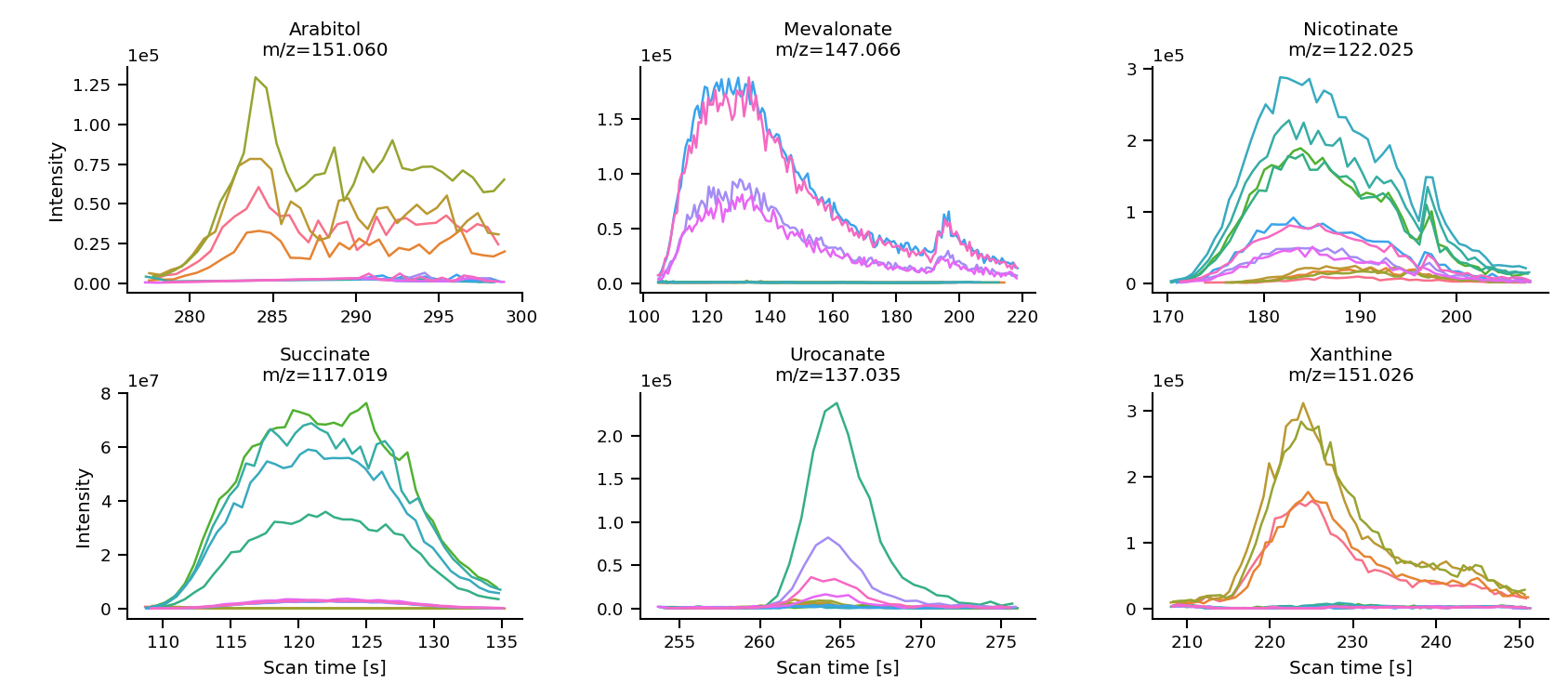
142
|
|
|
141
143
|
Now, we can run the peak optimization with:
|
|
142
144
|
|
|
@@ -153,7 +155,7 @@ If you do not provide a list of peak_labels to the `mint.opt.rt_min_max()` funct
|
|
|
153
155
|
|
|
154
156
|
After running the optimization, it is a good idea to perform a manual fine-tuning of the `rt_min` and `rt_max` values, especially for complicated peaks (peaks with multiple components, noisy peaks, etc.). You can use the `mint.plot.peak_shapes()` function to visualize the peak shapes and identify any areas that may require further attention.
|
|
155
157
|
|
|
156
|
-

|
|
158
|
+

|
|
157
159
|
|
|
158
160
|
The black lines indicates the average intensity across all files used for the optimization. The orange dotted lines show the shape of the gaussian function used to weight the mean intensities for peak selection. The orange horizontal lines indicate the peak width and the blue `x`s show the identified peak maxima. The green shaded areas show the Rt ranges which were selected by the algorithm.
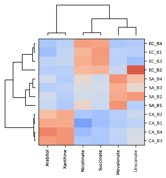
|
|
159
161
|
|
|
@@ -162,7 +164,7 @@ Then we apply the changes and plot the new peak shapes:
|
|
|
162
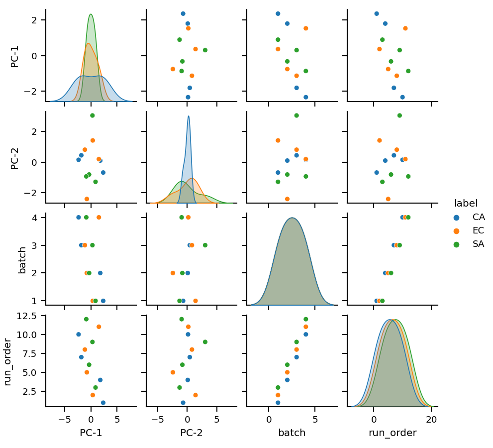
164
|
mint.run()
|
|
163
165
|
mint.plot.peak_shapes(col_wrap=3)
|
|
164
166
|
|
|
165
|
-

|
|
167
|
+

|
|
166
168
|
|
|
167
169
|
As you can see, the shapes of Xanthine, Succinate, Citrulline look much better.
|
|
168
170
|
|
|
@@ -172,7 +174,7 @@ The `Mint` class has a few convenient methods to visualize and explore the proce
|
|
|
172
174
|
|
|
173
175
|
## Plot peak shapes
|
|
174
176
|
|
|
175
|
-

|
|
177
|
+

|
|
176
178
|
|
|
177
179
|
mint.plot.peak_shapes(col_wrap = 3)
|
|
178
180
|
|
|
@@ -207,7 +209,7 @@ Before clustering the data can be transformed and scaled. By default `log2p1(x)
|
|
|
207
209
|
cmap=None # Name of a matplotlib color map
|
|
208
210
|
)
|
|
209
211
|
|
|
210
|
-

|
|
212
|
+
|
|
211
213
|
|
|
212
214
|
## Principal Components Analysis
|
|
213
215
|
|
|
@@ -221,7 +223,7 @@ After running the PCA the results can be plotted with:
|
|
|
221
223
|
|
|
222
224
|
mint.pca.plot.pairplot(n_components=5, interactive=False)
|
|
223
225
|
|
|
224
|
-

|
|
226
|
+
|
|
225
227
|
|
|
226
228
|
## FAQ
|
|
227
229
|
### What is a target list
|
|
@@ -1,6 +1,8 @@
|
|
|
1
1
|
[](https://github.com/LewisResearchGroup/ms-mint/actions/workflows/pythonpackage.yml)
|
|
2
2
|

|
|
3
3
|
[](https://github.com/lewisresearchgroup/ms-mint/actions/workflows/codeql-analysis.yml)
|
|
4
|
+

|
|
5
|
+

|
|
4
6
|
|
|
5
7
|
# Wecome to ms-mint
|
|
6
8
|
|
|
@@ -122,7 +124,7 @@ If you only have retention time (Rt) values for your targets, or if the Rt value
|
|
|
122
124
|
|
|
123
125
|
To use the `mint.opt.rt_min_max()` function, you will need to provide it with a list of retention times for your targets and the names of the mass spectrometry files containing your data. The function will then search through the data to find the optimal `rt_min` and `rt_max` values, which you can use to refine your analysis. You can then use these optimized values in conjunction with the other functions and methods of the `Mint` class to process and analyze your data.
|
|
124
126
|
|
|
125
|
-

|
|
127
|
+

|
|
126
128
|
|
|
127
129
|
Now, we can run the peak optimization with:
|
|
128
130
|
|
|
@@ -139,7 +141,7 @@ If you do not provide a list of peak_labels to the `mint.opt.rt_min_max()` funct
|
|
|
139
141
|
|
|
140
142
|
After running the optimization, it is a good idea to perform a manual fine-tuning of the `rt_min` and `rt_max` values, especially for complicated peaks (peaks with multiple components, noisy peaks, etc.). You can use the `mint.plot.peak_shapes()` function to visualize the peak shapes and identify any areas that may require further attention.
|
|
141
143
|
|
|
142
|
-

|
|
144
|
+

|
|
143
145
|
|
|
144
146
|
The black lines indicates the average intensity across all files used for the optimization. The orange dotted lines show the shape of the gaussian function used to weight the mean intensities for peak selection. The orange horizontal lines indicate the peak width and the blue `x`s show the identified peak maxima. The green shaded areas show the Rt ranges which were selected by the algorithm.
|
|
145
147
|
|
|
@@ -148,7 +150,7 @@ Then we apply the changes and plot the new peak shapes:
|
|
|
148
150
|
mint.run()
|
|
149
151
|
mint.plot.peak_shapes(col_wrap=3)
|
|
150
152
|
|
|
151
|
-

|
|
153
|
+

|
|
152
154
|
|
|
153
155
|
As you can see, the shapes of Xanthine, Succinate, Citrulline look much better.
|
|
154
156
|
|
|
@@ -158,7 +160,7 @@ The `Mint` class has a few convenient methods to visualize and explore the proce
|
|
|
158
160
|
|
|
159
161
|
## Plot peak shapes
|
|
160
162
|
|
|
161
|
-

|
|
163
|
+

|
|
162
164
|
|
|
163
165
|
mint.plot.peak_shapes(col_wrap = 3)
|
|
164
166
|
|
|
@@ -193,7 +195,7 @@ Before clustering the data can be transformed and scaled. By default `log2p1(x)
|
|
|
193
195
|
cmap=None # Name of a matplotlib color map
|
|
194
196
|
)
|
|
195
197
|
|
|
196
|
-

|
|
198
|
+

|
|
197
199
|
|
|
198
200
|
## Principal Components Analysis
|
|
199
201
|
|
|
@@ -207,7 +209,7 @@ After running the PCA the results can be plotted with:
|
|
|
207
209
|
|
|
208
210
|
mint.pca.plot.pairplot(n_components=5, interactive=False)
|
|
209
211
|
|
|
210
|
-

|
|
212
|
+

|
|
211
213
|
|
|
212
214
|
## FAQ
|
|
213
215
|
### What is a target list
|
|
@@ -133,11 +133,11 @@ class MintPlotter:
|
|
|
133
133
|
if len(self.mint.results) > 0:
|
|
134
134
|
if not interactive:
|
|
135
135
|
return plot_peak_shapes(
|
|
136
|
-
self.mint.results, fns=fns, peak_labels=peak_labels, **kwargs
|
|
136
|
+
self.mint.results, mint_metadata=self.mint.meta, fns=fns, peak_labels=peak_labels, **kwargs
|
|
137
137
|
)
|
|
138
138
|
else:
|
|
139
139
|
return plotly_peak_shapes(
|
|
140
|
-
self.mint.results, fns=fns, peak_labels=peak_labels, **kwargs
|
|
140
|
+
self.mint.results, mint_metadata=self.mint.meta, fns=fns, peak_labels=peak_labels, **kwargs
|
|
141
141
|
)
|
|
142
142
|
|
|
143
143
|
def heatmap(
|
|
@@ -8,11 +8,11 @@ import json
|
|
|
8
8
|
|
|
9
9
|
version_json = '''
|
|
10
10
|
{
|
|
11
|
-
"date": "2023-
|
|
11
|
+
"date": "2023-08-18T12:58:02-0600",
|
|
12
12
|
"dirty": false,
|
|
13
13
|
"error": null,
|
|
14
|
-
"full-revisionid": "
|
|
15
|
-
"version": "v0.3.
|
|
14
|
+
"full-revisionid": "2563246318a0e00988500da34daed80721f81b98",
|
|
15
|
+
"version": "v0.3.2"
|
|
16
16
|
}
|
|
17
17
|
''' # END VERSION_JSON
|
|
18
18
|
|
|
@@ -130,17 +130,19 @@ def hierarchical_clustering(
|
|
|
130
130
|
|
|
131
131
|
def plot_peak_shapes(
|
|
132
132
|
mint_results,
|
|
133
|
+
mint_metadata=None,
|
|
133
134
|
fns=None,
|
|
134
135
|
peak_labels=None,
|
|
135
136
|
height=3,
|
|
136
137
|
aspect=1.5,
|
|
137
138
|
legend=False,
|
|
138
139
|
col_wrap=4,
|
|
139
|
-
hue="
|
|
140
|
+
hue="ms_file_label",
|
|
140
141
|
title=None,
|
|
141
142
|
dpi=None,
|
|
142
143
|
sharex=False,
|
|
143
144
|
sharey=False,
|
|
145
|
+
kind='line',
|
|
144
146
|
**kwargs,
|
|
145
147
|
):
|
|
146
148
|
"""
|
|
@@ -148,6 +150,8 @@ def plot_peak_shapes(
|
|
|
148
150
|
|
|
149
151
|
:param mint_results: DataFrame in Mint results format.
|
|
150
152
|
:type mint_results: pandas.DataFrame
|
|
153
|
+
:param mint_metadata: DataFrame in Mint metadata format.
|
|
154
|
+
:type mint_metadata: pandas.DataFrame
|
|
151
155
|
:param fns: Filenames to include, defaults to None
|
|
152
156
|
:type fns: list, optional
|
|
153
157
|
:param peak_labels: Peak-labels to include, defaults to None
|
|
@@ -170,6 +174,8 @@ def plot_peak_shapes(
|
|
|
170
174
|
:type sharex: bool, optional
|
|
171
175
|
:param sharey: Whether or not to share y-axis range between subplots, defaults to False
|
|
172
176
|
:type sharey: bool, optional
|
|
177
|
+
:param kind: Kind of seaborn relplot
|
|
178
|
+
:type kind: str, optional
|
|
173
179
|
:return: Generated figure object.
|
|
174
180
|
:rtype: matplotlib.pyplot.Figure
|
|
175
181
|
"""
|
|
@@ -197,7 +203,7 @@ def plot_peak_shapes(
|
|
|
197
203
|
].iterrows():
|
|
198
204
|
peak_rt = [float(i) for i in row.peak_shape_rt.split(",")]
|
|
199
205
|
peak_int = [float(i) for i in row.peak_shape_int.split(",")]
|
|
200
|
-
|
|
206
|
+
ms_file_label = row.ms_file_label
|
|
201
207
|
mz = row.mz_mean
|
|
202
208
|
rt = row.rt
|
|
203
209
|
|
|
@@ -205,7 +211,7 @@ def plot_peak_shapes(
|
|
|
205
211
|
{
|
|
206
212
|
"Scan time [s]": peak_rt,
|
|
207
213
|
"Intensity": peak_int,
|
|
208
|
-
"
|
|
214
|
+
"ms_file_label": ms_file_label,
|
|
209
215
|
"peak_label": peak_label + f"\nm/z={mz:.3f}",
|
|
210
216
|
"Expected Scan time [s]": rt,
|
|
211
217
|
}
|
|
@@ -214,13 +220,17 @@ def plot_peak_shapes(
|
|
|
214
220
|
|
|
215
221
|
df = pd.concat(dfs).reset_index(drop=True)
|
|
216
222
|
|
|
223
|
+
# Add metadata
|
|
224
|
+
if mint_metadata is not None:
|
|
225
|
+
df = pd.merge(df, mint_metadata, left_on='ms_file_label', right_index=True)
|
|
226
|
+
|
|
217
227
|
g = sns.relplot(
|
|
218
228
|
data=df,
|
|
219
229
|
x="Scan time [s]",
|
|
220
230
|
y="Intensity",
|
|
221
231
|
hue=hue,
|
|
222
232
|
col="peak_label",
|
|
223
|
-
kind=
|
|
233
|
+
kind=kind,
|
|
224
234
|
col_wrap=col_wrap,
|
|
225
235
|
height=height,
|
|
226
236
|
aspect=aspect,
|
|
@@ -1,6 +1,7 @@
|
|
|
1
1
|
import logging
|
|
2
2
|
|
|
3
3
|
import numpy as np
|
|
4
|
+
import pandas as pd
|
|
4
5
|
import colorlover as cl
|
|
5
6
|
|
|
6
7
|
import plotly.graph_objects as go
|
|
@@ -222,6 +223,8 @@ def plotly_heatmap(
|
|
|
222
223
|
|
|
223
224
|
def plotly_peak_shapes(
|
|
224
225
|
mint_results,
|
|
226
|
+
mint_metadata=None,
|
|
227
|
+
color='ms_file_label', # Add the new argument for specifying color column
|
|
225
228
|
fns=None,
|
|
226
229
|
col_wrap=1,
|
|
227
230
|
peak_labels=None,
|
|
@@ -229,52 +232,90 @@ def plotly_peak_shapes(
|
|
|
229
232
|
verbose=False,
|
|
230
233
|
legend_orientation="v",
|
|
231
234
|
call_show=False,
|
|
235
|
+
palette='Plasma',
|
|
232
236
|
):
|
|
233
|
-
"""
|
|
234
|
-
|
|
235
|
-
|
|
237
|
+
"""
|
|
238
|
+
Plot peak shapes of mint results.
|
|
239
|
+
|
|
240
|
+
:param mint_results: DataFrame in Mint results format.
|
|
241
|
+
:type mint_results: pandas.DataFrame
|
|
242
|
+
:param mint_metadata: DataFrame in Mint metadata format, defaults to None.
|
|
243
|
+
:type mint_metadata: pandas.DataFrame, optional
|
|
244
|
+
:param color: Column name determining color-coding of plots, defaults to 'ms_file_label'.
|
|
245
|
+
:type color: str, optional
|
|
246
|
+
:param fns: Filenames to include, defaults to None.
|
|
247
|
+
:type fns: list, optional
|
|
248
|
+
:param col_wrap: Maximum number of subplot columns, defaults to 1.
|
|
249
|
+
:type col_wrap: int, optional
|
|
250
|
+
:param peak_labels: Peak-labels to include, defaults to None.
|
|
251
|
+
:type peak_labels: list, optional
|
|
252
|
+
:param legend: Whether to display legend, defaults to True.
|
|
253
|
+
:type legend: bool, optional
|
|
254
|
+
:param verbose: If True, prints additional details, defaults to False.
|
|
255
|
+
:type verbose: bool, optional
|
|
256
|
+
:param legend_orientation: Legend orientation, defaults to 'v'.
|
|
257
|
+
:type legend_orientation: str, optional
|
|
258
|
+
:param call_show: If True, displays the plot immediately, defaults to False.
|
|
259
|
+
:type call_show: bool, optional
|
|
260
|
+
:param palette: Color palette to use, defaults to 'Plasma'.
|
|
261
|
+
:type palette: str, optional
|
|
262
|
+
|
|
263
|
+
:return: Plotly Figure object or None if call_show is True.
|
|
264
|
+
:rtype: plotly.graph_objs._figure.Figure or None
|
|
236
265
|
"""
|
|
237
266
|
mint_results = mint_results.copy()
|
|
238
267
|
|
|
268
|
+
# Merge with metadata if provided
|
|
269
|
+
if mint_metadata is not None:
|
|
270
|
+
mint_results = pd.merge(mint_results, mint_metadata, left_on='ms_file_label', right_index=True)
|
|
239
271
|
|
|
272
|
+
# Filter by filenames
|
|
240
273
|
if fns is not None:
|
|
241
274
|
fns = [fn_to_label(fn) for fn in fns]
|
|
242
275
|
mint_results = mint_results[mint_results.ms_file_label.isin(fns)]
|
|
276
|
+
else:
|
|
277
|
+
fns = mint_results.ms_file_label.unique()
|
|
278
|
+
|
|
279
|
+
# Filter by peak_labels
|
|
280
|
+
if peak_labels is not None:
|
|
281
|
+
if isinstance(peak_labels, str):
|
|
282
|
+
peak_labels = [peak_labels]
|
|
283
|
+
mint_results = mint_results[mint_results.peak_label.isin(peak_labels)]
|
|
284
|
+
else:
|
|
285
|
+
peak_labels = mint_results.results.peak_label.unique()
|
|
286
|
+
|
|
287
|
+
# Handle colors based on metadata or fall back to default behavior
|
|
288
|
+
colors = None
|
|
289
|
+
if color:
|
|
290
|
+
unique_hues = mint_results[color].unique()
|
|
291
|
+
|
|
292
|
+
colors = get_palette_colors(palette, len(unique_hues))
|
|
293
|
+
|
|
294
|
+
color_mapping = dict(zip(unique_hues, colors))
|
|
295
|
+
|
|
296
|
+
if color == 'ms_file_label':
|
|
297
|
+
hue_column = [color_mapping[fn] for fn in fns]
|
|
298
|
+
else:
|
|
299
|
+
# Existing logic remains the same for the else part
|
|
300
|
+
hue_column = mint_results.drop_duplicates('ms_file_label').set_index('ms_file_label')[color].map(color_mapping).reindex(fns).tolist()
|
|
243
301
|
|
|
244
|
-
|
|
245
|
-
|
|
246
|
-
logging.warning("TEST")
|
|
302
|
+
else:
|
|
303
|
+
hue_column = colors
|
|
247
304
|
|
|
305
|
+
# Rest of the plotting process
|
|
248
306
|
res = mint_results[mint_results.peak_max > 0]
|
|
249
|
-
|
|
250
|
-
fns = res.ms_file_label.unique()
|
|
251
307
|
labels = mint_results.peak_label.unique()
|
|
252
|
-
|
|
253
308
|
res = res.set_index(["peak_label", "ms_file_label"]).sort_index()
|
|
254
309
|
|
|
255
|
-
|
|
256
|
-
peak_labels = [peak_labels]
|
|
257
|
-
|
|
258
|
-
# Calculate neccessary number of rows
|
|
310
|
+
# Calculate necessary number of rows
|
|
259
311
|
n_rows = max(1, len(labels) // col_wrap)
|
|
260
312
|
if n_rows * col_wrap < len(labels):
|
|
261
313
|
n_rows += 1
|
|
262
314
|
|
|
263
|
-
if verbose:
|
|
264
|
-
print(n_rows, col_wrap)
|
|
265
|
-
print("ms_files:", fns)
|
|
266
|
-
print("peak_labels:", peak_labels)
|
|
267
|
-
print("Data:", res)
|
|
268
|
-
|
|
269
315
|
fig = make_subplots(
|
|
270
316
|
rows=max(1, n_rows), cols=max(1, col_wrap), subplot_titles=peak_labels
|
|
271
317
|
)
|
|
272
|
-
if len(fns) < 13:
|
|
273
|
-
colors = cl.scales["12"]["qual"]["Paired"]
|
|
274
|
-
else:
|
|
275
|
-
colors = cl.interp(cl.scales["12"]["qual"]["Paired"], len(fns))
|
|
276
318
|
|
|
277
|
-
# Create sub-plots
|
|
278
319
|
for label_i, label in enumerate(peak_labels):
|
|
279
320
|
for file_i, fn in enumerate(fns):
|
|
280
321
|
try:
|
|
@@ -282,9 +323,9 @@ def plotly_peak_shapes(
|
|
|
282
323
|
except KeyError as e:
|
|
283
324
|
logging.warning(e)
|
|
284
325
|
continue
|
|
326
|
+
|
|
285
327
|
if not isinstance(x, Iterable):
|
|
286
328
|
continue
|
|
287
|
-
|
|
288
329
|
if isinstance(x, str):
|
|
289
330
|
x = x.split(",")
|
|
290
331
|
y = y.split(",")
|
|
@@ -297,6 +338,8 @@ def plotly_peak_shapes(
|
|
|
297
338
|
else:
|
|
298
339
|
mode = "lines"
|
|
299
340
|
|
|
341
|
+
trace_color = trace_color = hue_column[file_i]
|
|
342
|
+
|
|
300
343
|
fig.add_trace(
|
|
301
344
|
go.Scatter(
|
|
302
345
|
x=x,
|
|
@@ -305,7 +348,7 @@ def plotly_peak_shapes(
|
|
|
305
348
|
mode=mode,
|
|
306
349
|
legendgroup=file_i,
|
|
307
350
|
showlegend=(label_i == 0),
|
|
308
|
-
marker_color=
|
|
351
|
+
marker_color=trace_color,
|
|
309
352
|
text=fn,
|
|
310
353
|
),
|
|
311
354
|
row=ndx_r,
|
|
@@ -315,10 +358,10 @@ def plotly_peak_shapes(
|
|
|
315
358
|
fig.update_xaxes(title_text="Scan time [s]", row=ndx_r, col=ndx_c)
|
|
316
359
|
fig.update_yaxes(title_text="Intensity", row=ndx_r, col=ndx_c)
|
|
317
360
|
|
|
318
|
-
# Layout
|
|
361
|
+
# Layout updates
|
|
319
362
|
if legend:
|
|
320
363
|
fig.update_layout(legend_orientation=legend_orientation)
|
|
321
|
-
|
|
364
|
+
|
|
322
365
|
fig.update_layout(showlegend=legend)
|
|
323
366
|
fig.update_layout(height=400 * n_rows, title_text="Peak Shapes")
|
|
324
367
|
|
|
@@ -326,3 +369,17 @@ def plotly_peak_shapes(
|
|
|
326
369
|
fig.show(config={"displaylogo": False})
|
|
327
370
|
else:
|
|
328
371
|
return fig
|
|
372
|
+
|
|
373
|
+
|
|
374
|
+
def get_palette_colors(palette_name, num_colors):
|
|
375
|
+
# Categories in the colorlover package
|
|
376
|
+
categories = ["qual", "seq", "div"]
|
|
377
|
+
|
|
378
|
+
num_colors = max(num_colors, 3)
|
|
379
|
+
# Check in which category our palette resides
|
|
380
|
+
for category in categories:
|
|
381
|
+
if palette_name in cl.scales[f"{num_colors}"][category]:
|
|
382
|
+
return cl.scales[f"{num_colors}"][category][palette_name]
|
|
383
|
+
|
|
384
|
+
# If palette not found in any category, return a default one or raise an error
|
|
385
|
+
return cl.scales[f"{num_colors}"]["qual"]["Paired"]
|
|
@@ -58,4 +58,18 @@ DEPRECATED_LABELS = {
|
|
|
58
58
|
"ms_file_size": "ms_file_size_MB",
|
|
59
59
|
}
|
|
60
60
|
|
|
61
|
+
MINT_METADATA_COLUMNS = [
|
|
62
|
+
'ms_file_label',
|
|
63
|
+
'label',
|
|
64
|
+
'group',
|
|
65
|
+
'batch',
|
|
66
|
+
'sample_type',
|
|
67
|
+
'run_order',
|
|
68
|
+
'plate',
|
|
69
|
+
'plate_row',
|
|
70
|
+
'plate_col',
|
|
71
|
+
'lc_column',
|
|
72
|
+
'polarity'
|
|
73
|
+
]
|
|
74
|
+
|
|
61
75
|
M_PROTON = 1.00782503223
|
|
@@ -8,7 +8,7 @@ from molmass import Formula, FormulaError
|
|
|
8
8
|
from sklearn.preprocessing import MinMaxScaler, StandardScaler, RobustScaler
|
|
9
9
|
from scipy.signal import find_peaks, peak_widths
|
|
10
10
|
|
|
11
|
-
from .standards import M_PROTON, TARGETS_COLUMNS
|
|
11
|
+
from .standards import M_PROTON, TARGETS_COLUMNS, MINT_METADATA_COLUMNS
|
|
12
12
|
from .filelock import FileLock
|
|
13
13
|
from .matplotlib_tools import plot_peaks
|
|
14
14
|
|
|
@@ -230,18 +230,9 @@ def mz_mean_width_to_min_max(mz_mean, mz_width):
|
|
|
230
230
|
mz_max = mz_mean + delta_mass
|
|
231
231
|
return mz_min, mz_max
|
|
232
232
|
|
|
233
|
+
|
|
233
234
|
def init_metadata():
|
|
234
|
-
cols =
|
|
235
|
-
'ms_file_label',
|
|
236
|
-
'ms_file',
|
|
237
|
-
'label',
|
|
238
|
-
'group',
|
|
239
|
-
'type',
|
|
240
|
-
'run_order',
|
|
241
|
-
'plate',
|
|
242
|
-
'plate_row',
|
|
243
|
-
'plate_col'
|
|
244
|
-
]
|
|
235
|
+
cols = MINT_METADATA_COLUMNS
|
|
245
236
|
return pd.DataFrame(columns=cols).set_index('ms_file_label')
|
|
246
237
|
|
|
247
238
|
|
|
@@ -1,6 +1,6 @@
|
|
|
1
1
|
Metadata-Version: 2.1
|
|
2
2
|
Name: ms-mint
|
|
3
|
-
Version: 0.3.
|
|
3
|
+
Version: 0.3.2
|
|
4
4
|
Summary: Metabolomics Integrator (Mint)
|
|
5
5
|
Home-page: https://github.com/LewisResearchGroup/ms-mint
|
|
6
6
|
Author: Soren Wacker
|
|
@@ -15,6 +15,8 @@ License-File: LICENSE
|
|
|
15
15
|
[](https://github.com/LewisResearchGroup/ms-mint/actions/workflows/pythonpackage.yml)
|
|
16
16
|

|
|
17
17
|
[](https://github.com/lewisresearchgroup/ms-mint/actions/workflows/codeql-analysis.yml)
|
|
18
|
+

|
|
19
|
+

|
|
18
20
|
|
|
19
21
|
# Wecome to ms-mint
|
|
20
22
|
|
|
@@ -136,7 +138,7 @@ If you only have retention time (Rt) values for your targets, or if the Rt value
|
|
|
136
138
|
|
|
137
139
|
To use the `mint.opt.rt_min_max()` function, you will need to provide it with a list of retention times for your targets and the names of the mass spectrometry files containing your data. The function will then search through the data to find the optimal `rt_min` and `rt_max` values, which you can use to refine your analysis. You can then use these optimized values in conjunction with the other functions and methods of the `Mint` class to process and analyze your data.
|
|
138
140
|
|
|
139
|
-

|
|
141
|
+

|
|
140
142
|
|
|
141
143
|
Now, we can run the peak optimization with:
|
|
142
144
|
|
|
@@ -153,7 +155,7 @@ If you do not provide a list of peak_labels to the `mint.opt.rt_min_max()` funct
|
|
|
153
155
|
|
|
154
156
|
After running the optimization, it is a good idea to perform a manual fine-tuning of the `rt_min` and `rt_max` values, especially for complicated peaks (peaks with multiple components, noisy peaks, etc.). You can use the `mint.plot.peak_shapes()` function to visualize the peak shapes and identify any areas that may require further attention.
|
|
155
157
|
|
|
156
|
-

|
|
158
|
+

|
|
157
159
|
|
|
158
160
|
The black lines indicates the average intensity across all files used for the optimization. The orange dotted lines show the shape of the gaussian function used to weight the mean intensities for peak selection. The orange horizontal lines indicate the peak width and the blue `x`s show the identified peak maxima. The green shaded areas show the Rt ranges which were selected by the algorithm.
|
|
159
161
|
|
|
@@ -162,7 +164,7 @@ Then we apply the changes and plot the new peak shapes:
|
|
|
162
164
|
mint.run()
|
|
163
165
|
mint.plot.peak_shapes(col_wrap=3)
|
|
164
166
|
|
|
165
|
-

|
|
167
|
+

|
|
166
168
|
|
|
167
169
|
As you can see, the shapes of Xanthine, Succinate, Citrulline look much better.
|
|
168
170
|
|
|
@@ -172,7 +174,7 @@ The `Mint` class has a few convenient methods to visualize and explore the proce
|
|
|
172
174
|
|
|
173
175
|
## Plot peak shapes
|
|
174
176
|
|
|
175
|
-

|
|
177
|
+

|
|
176
178
|
|
|
177
179
|
mint.plot.peak_shapes(col_wrap = 3)
|
|
178
180
|
|
|
@@ -207,7 +209,7 @@ Before clustering the data can be transformed and scaled. By default `log2p1(x)
|
|
|
207
209
|
cmap=None # Name of a matplotlib color map
|
|
208
210
|
)
|
|
209
211
|
|
|
210
|
-

|
|
212
|
+

|
|
211
213
|
|
|
212
214
|
## Principal Components Analysis
|
|
213
215
|
|
|
@@ -221,7 +223,7 @@ After running the PCA the results can be plotted with:
|
|
|
221
223
|
|
|
222
224
|
mint.pca.plot.pairplot(n_components=5, interactive=False)
|
|
223
225
|
|
|
224
|
-

|
|
226
|
+

|
|
225
227
|
|
|
226
228
|
## FAQ
|
|
227
229
|
### What is a target list
|
|
File without changes
|
|
File without changes
|
|
File without changes
|
|
File without changes
|
|
File without changes
|
|
File without changes
|
|
File without changes
|
|
File without changes
|
|
File without changes
|
|
File without changes
|
|
File without changes
|
|
File without changes
|
|
File without changes
|
|
File without changes
|
|
File without changes
|
|
File without changes
|
|
File without changes
|
|
File without changes
|
|
File without changes
|
|
File without changes
|
|
File without changes
|