molscope 0.6.2__tar.gz → 0.7.0__tar.gz
This diff represents the content of publicly available package versions that have been released to one of the supported registries. The information contained in this diff is provided for informational purposes only and reflects changes between package versions as they appear in their respective public registries.
- {molscope-0.6.2 → molscope-0.7.0}/PKG-INFO +56 -4
- {molscope-0.6.2 → molscope-0.7.0}/README.md +55 -3
- {molscope-0.6.2 → molscope-0.7.0}/molscope/__init__.py +5 -2
- molscope-0.7.0/molscope/dssp.py +232 -0
- {molscope-0.6.2 → molscope-0.7.0}/molscope/molecule.py +13 -0
- {molscope-0.6.2 → molscope-0.7.0}/molscope/plotting.py +7 -2
- {molscope-0.6.2 → molscope-0.7.0}/molscope.egg-info/PKG-INFO +56 -4
- {molscope-0.6.2 → molscope-0.7.0}/molscope.egg-info/SOURCES.txt +2 -0
- {molscope-0.6.2 → molscope-0.7.0}/pyproject.toml +3 -1
- molscope-0.7.0/tests/test_dssp.py +67 -0
- {molscope-0.6.2 → molscope-0.7.0}/LICENSE +0 -0
- {molscope-0.6.2 → molscope-0.7.0}/molscope/__main__.py +0 -0
- {molscope-0.6.2 → molscope-0.7.0}/molscope/cli.py +0 -0
- {molscope-0.6.2 → molscope-0.7.0}/molscope/coarsegrain.py +0 -0
- {molscope-0.6.2 → molscope-0.7.0}/molscope/contactmap.py +0 -0
- {molscope-0.6.2 → molscope-0.7.0}/molscope/descriptors.py +0 -0
- {molscope-0.6.2 → molscope-0.7.0}/molscope/elements.py +0 -0
- {molscope-0.6.2 → molscope-0.7.0}/molscope/ensemble.py +0 -0
- {molscope-0.6.2 → molscope-0.7.0}/molscope/graph.py +0 -0
- {molscope-0.6.2 → molscope-0.7.0}/molscope/io.py +0 -0
- {molscope-0.6.2 → molscope-0.7.0}/molscope.egg-info/dependency_links.txt +0 -0
- {molscope-0.6.2 → molscope-0.7.0}/molscope.egg-info/entry_points.txt +0 -0
- {molscope-0.6.2 → molscope-0.7.0}/molscope.egg-info/requires.txt +0 -0
- {molscope-0.6.2 → molscope-0.7.0}/molscope.egg-info/top_level.txt +0 -0
- {molscope-0.6.2 → molscope-0.7.0}/setup.cfg +0 -0
- {molscope-0.6.2 → molscope-0.7.0}/tests/test_clustering.py +0 -0
- {molscope-0.6.2 → molscope-0.7.0}/tests/test_coarsegrain.py +0 -0
- {molscope-0.6.2 → molscope-0.7.0}/tests/test_contactmap.py +0 -0
- {molscope-0.6.2 → molscope-0.7.0}/tests/test_descriptors.py +0 -0
- {molscope-0.6.2 → molscope-0.7.0}/tests/test_features.py +0 -0
- {molscope-0.6.2 → molscope-0.7.0}/tests/test_graph.py +0 -0
- {molscope-0.6.2 → molscope-0.7.0}/tests/test_io.py +0 -0
- {molscope-0.6.2 → molscope-0.7.0}/tests/test_molecule.py +0 -0
|
@@ -1,6 +1,6 @@
|
|
|
1
1
|
Metadata-Version: 2.4
|
|
2
2
|
Name: molscope
|
|
3
|
-
Version: 0.
|
|
3
|
+
Version: 0.7.0
|
|
4
4
|
Summary: Lightweight molecular structure analysis, visualisation, graph export, and coarse-graining in Python.
|
|
5
5
|
Author-email: Roshan Shrestha <roshanpra@gmail.com>
|
|
6
6
|
License-Expression: MIT
|
|
@@ -38,9 +38,9 @@ coarse-graining in Python. Read `.xyz`, `.pdb`, `.cif` and `.sdf` files
|
|
|
38
38
|
3D. The `.cif` reader is a basic mmCIF parser for standard `_atom_site`
|
|
39
39
|
coordinate loops, not a full mmCIF syntax implementation.
|
|
40
40
|
|
|
41
|
-
| 3D structure
|
|
42
|
-
| --- | --- | --- |
|
|
43
|
-
|  |  |  |
|
|
41
|
+
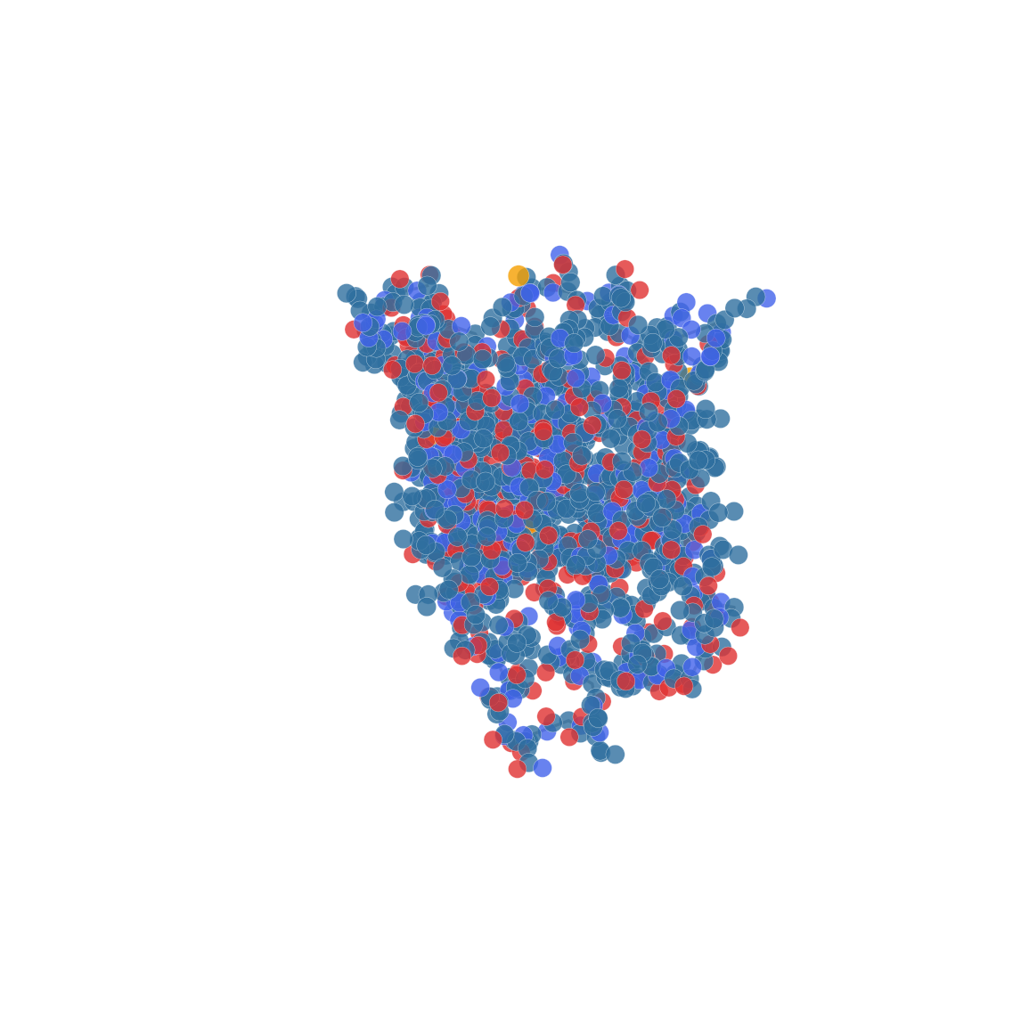
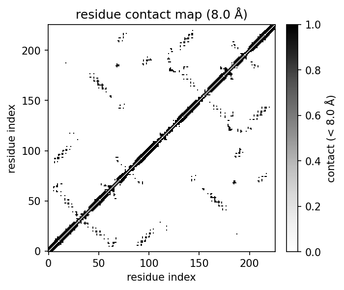
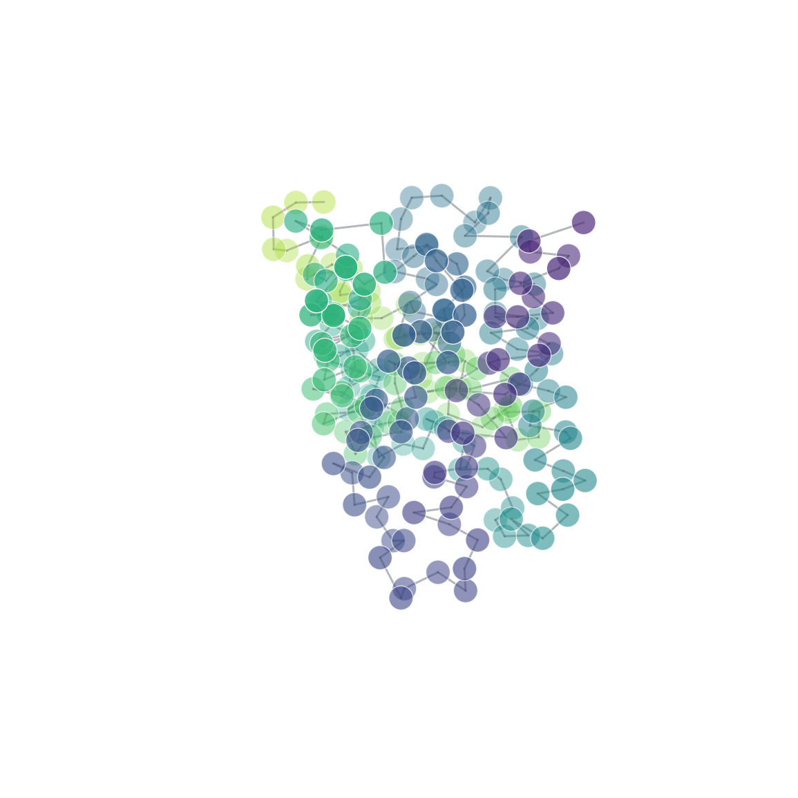
| 3D structure (element) | Secondary structure (DSSP) | Residue contact map | Coarse-grained beads |
|
|
42
|
+
| --- | --- | --- | --- |
|
|
43
|
+
|  |  |  |  |
|
|
44
44
|
|
|
45
45
|
## What it does
|
|
46
46
|
|
|
@@ -51,6 +51,8 @@ coordinate loops, not a full mmCIF syntax implementation.
|
|
|
51
51
|
- **Analyse** centroids, radius of gyration, the inertia tensor, inferred bonds
|
|
52
52
|
and contacts.
|
|
53
53
|
- **Contact maps** at atom or residue level, with heatmap plots.
|
|
54
|
+
- **Secondary structure** via a self-contained, dependency-free DSSP, with
|
|
55
|
+
`plot(color_by="ss")`.
|
|
54
56
|
- **Ensembles**: pairwise RMSD, RMSF, averaging, and conformer clustering.
|
|
55
57
|
- **Export for ML**: flat structural descriptors and molecular graphs for
|
|
56
58
|
NetworkX, PyTorch Geometric and DGL.
|
|
@@ -58,6 +60,33 @@ coordinate loops, not a full mmCIF syntax implementation.
|
|
|
58
60
|
- **Visualise** with 3D matplotlib plots, an interactive py3Dmol viewer, spin
|
|
59
61
|
GIFs, and a command-line interface.
|
|
60
62
|
|
|
63
|
+
## Why MolScope?
|
|
64
|
+
|
|
65
|
+
MolScope is **not** intended to replace full molecular-simulation or
|
|
66
|
+
cheminformatics frameworks. It is a lightweight **educational and prototyping**
|
|
67
|
+
toolkit for reading common molecular structure files, performing simple
|
|
68
|
+
structural analysis, exporting graph representations for ML workflows, and
|
|
69
|
+
experimenting with coarse-grained mappings. Its core depends only on NumPy and
|
|
70
|
+
Matplotlib, and the API is Python-first and scriptable.
|
|
71
|
+
|
|
72
|
+
In particular, the coarse-graining tools are for **educational CG mapping and
|
|
73
|
+
bead-graph prototyping**: useful for exploring mappings before moving to a
|
|
74
|
+
production Martini workflow. They are not a validated Martini force-field
|
|
75
|
+
generator.
|
|
76
|
+
|
|
77
|
+
| Tool | Main focus | How MolScope differs |
|
|
78
|
+
| --- | --- | --- |
|
|
79
|
+
| RDKit | Cheminformatics | MolScope leans toward structure visualisation, protein/PDB-style metadata, and CG prototyping |
|
|
80
|
+
| MDAnalysis | MD trajectories | MolScope is lighter and easier for static structures and teaching |
|
|
81
|
+
| MDTraj | Trajectory analysis | MolScope is simpler and graph/CG oriented |
|
|
82
|
+
| Biopython | Structure parsing / bioinformatics | MolScope adds 3D analysis, ML-graph export, and coarse-graining |
|
|
83
|
+
| PyMOL / VMD | Interactive visualisation | MolScope is Python-first, scriptable, and ML-export friendly |
|
|
84
|
+
| nglview | Notebook structure viewer | MolScope also does analysis, descriptors, graphs and CG, not just viewing |
|
|
85
|
+
|
|
86
|
+
Reach for those tools when you need their depth and validation. Reach for
|
|
87
|
+
MolScope when you want something small, readable, and quick to teach or
|
|
88
|
+
prototype with.
|
|
89
|
+
|
|
61
90
|
## Install
|
|
62
91
|
|
|
63
92
|
With [uv](https://docs.astral.sh/uv/) (recommended):
|
|
@@ -184,6 +213,29 @@ mol.contact_map(level="residue", method="min") # closest inter-residue at
|
|
|
184
213
|
mol.contact_map(level="residue", method="com") # residue centre of mass
|
|
185
214
|
```
|
|
186
215
|
|
|
216
|
+
### Secondary structure (DSSP)
|
|
217
|
+
|
|
218
|
+
Assign protein secondary structure from backbone hydrogen-bond patterns with a
|
|
219
|
+
self-contained, pure-NumPy DSSP (no external `mkdssp` binary needed):
|
|
220
|
+
|
|
221
|
+
```python
|
|
222
|
+
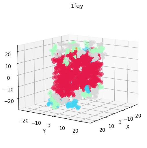
mol = ms.read("1fqy.pdb")
|
|
223
|
+
ss = mol.secondary_structure() # SecondaryStructure, one code per residue
|
|
224
|
+
|
|
225
|
+
ss.string # e.g. '--HHHHHHHH--SS--EEEE--'
|
|
226
|
+
ss.codes # per-residue array
|
|
227
|
+
ss.summary() # helix/strand/coil counts and fractions
|
|
228
|
+
|
|
229
|
+
mol.plot(color_by="ss") # colour the 3D view by secondary structure
|
|
230
|
+
```
|
|
231
|
+
|
|
232
|
+
Codes follow DSSP: `H`/`G`/`I` helices, `E`/`B` strands, `T` turn, `S` bend,
|
|
233
|
+
`-` coil. This is a simplified **educational** implementation: it reproduces the
|
|
234
|
+
main classes from the Kabsch-Sander hydrogen-bond model but is not bit-identical
|
|
235
|
+
to the reference `mkdssp` on every edge case. It needs backbone N/CA/C/O atoms,
|
|
236
|
+
so use PDB/mmCIF input (not a bare `.xyz`). The secondary-structure render in the
|
|
237
|
+
showcase above (helices red, turns cyan, coil grey) is produced this way.
|
|
238
|
+
|
|
187
239
|
### NMR ensembles
|
|
188
240
|
|
|
189
241
|
```python
|
|
@@ -11,9 +11,9 @@ coarse-graining in Python. Read `.xyz`, `.pdb`, `.cif` and `.sdf` files
|
|
|
11
11
|
3D. The `.cif` reader is a basic mmCIF parser for standard `_atom_site`
|
|
12
12
|
coordinate loops, not a full mmCIF syntax implementation.
|
|
13
13
|
|
|
14
|
-
| 3D structure
|
|
15
|
-
| --- | --- | --- |
|
|
16
|
-
|  |  |  |
|
|
14
|
+
| 3D structure (element) | Secondary structure (DSSP) | Residue contact map | Coarse-grained beads |
|
|
15
|
+
| --- | --- | --- | --- |
|
|
16
|
+
|  |  |  |  |
|
|
17
17
|
|
|
18
18
|
## What it does
|
|
19
19
|
|
|
@@ -24,6 +24,8 @@ coordinate loops, not a full mmCIF syntax implementation.
|
|
|
24
24
|
- **Analyse** centroids, radius of gyration, the inertia tensor, inferred bonds
|
|
25
25
|
and contacts.
|
|
26
26
|
- **Contact maps** at atom or residue level, with heatmap plots.
|
|
27
|
+
- **Secondary structure** via a self-contained, dependency-free DSSP, with
|
|
28
|
+
`plot(color_by="ss")`.
|
|
27
29
|
- **Ensembles**: pairwise RMSD, RMSF, averaging, and conformer clustering.
|
|
28
30
|
- **Export for ML**: flat structural descriptors and molecular graphs for
|
|
29
31
|
NetworkX, PyTorch Geometric and DGL.
|
|
@@ -31,6 +33,33 @@ coordinate loops, not a full mmCIF syntax implementation.
|
|
|
31
33
|
- **Visualise** with 3D matplotlib plots, an interactive py3Dmol viewer, spin
|
|
32
34
|
GIFs, and a command-line interface.
|
|
33
35
|
|
|
36
|
+
## Why MolScope?
|
|
37
|
+
|
|
38
|
+
MolScope is **not** intended to replace full molecular-simulation or
|
|
39
|
+
cheminformatics frameworks. It is a lightweight **educational and prototyping**
|
|
40
|
+
toolkit for reading common molecular structure files, performing simple
|
|
41
|
+
structural analysis, exporting graph representations for ML workflows, and
|
|
42
|
+
experimenting with coarse-grained mappings. Its core depends only on NumPy and
|
|
43
|
+
Matplotlib, and the API is Python-first and scriptable.
|
|
44
|
+
|
|
45
|
+
In particular, the coarse-graining tools are for **educational CG mapping and
|
|
46
|
+
bead-graph prototyping**: useful for exploring mappings before moving to a
|
|
47
|
+
production Martini workflow. They are not a validated Martini force-field
|
|
48
|
+
generator.
|
|
49
|
+
|
|
50
|
+
| Tool | Main focus | How MolScope differs |
|
|
51
|
+
| --- | --- | --- |
|
|
52
|
+
| RDKit | Cheminformatics | MolScope leans toward structure visualisation, protein/PDB-style metadata, and CG prototyping |
|
|
53
|
+
| MDAnalysis | MD trajectories | MolScope is lighter and easier for static structures and teaching |
|
|
54
|
+
| MDTraj | Trajectory analysis | MolScope is simpler and graph/CG oriented |
|
|
55
|
+
| Biopython | Structure parsing / bioinformatics | MolScope adds 3D analysis, ML-graph export, and coarse-graining |
|
|
56
|
+
| PyMOL / VMD | Interactive visualisation | MolScope is Python-first, scriptable, and ML-export friendly |
|
|
57
|
+
| nglview | Notebook structure viewer | MolScope also does analysis, descriptors, graphs and CG, not just viewing |
|
|
58
|
+
|
|
59
|
+
Reach for those tools when you need their depth and validation. Reach for
|
|
60
|
+
MolScope when you want something small, readable, and quick to teach or
|
|
61
|
+
prototype with.
|
|
62
|
+
|
|
34
63
|
## Install
|
|
35
64
|
|
|
36
65
|
With [uv](https://docs.astral.sh/uv/) (recommended):
|
|
@@ -157,6 +186,29 @@ mol.contact_map(level="residue", method="min") # closest inter-residue at
|
|
|
157
186
|
mol.contact_map(level="residue", method="com") # residue centre of mass
|
|
158
187
|
```
|
|
159
188
|
|
|
189
|
+
### Secondary structure (DSSP)
|
|
190
|
+
|
|
191
|
+
Assign protein secondary structure from backbone hydrogen-bond patterns with a
|
|
192
|
+
self-contained, pure-NumPy DSSP (no external `mkdssp` binary needed):
|
|
193
|
+
|
|
194
|
+
```python
|
|
195
|
+
mol = ms.read("1fqy.pdb")
|
|
196
|
+
ss = mol.secondary_structure() # SecondaryStructure, one code per residue
|
|
197
|
+
|
|
198
|
+
ss.string # e.g. '--HHHHHHHH--SS--EEEE--'
|
|
199
|
+
ss.codes # per-residue array
|
|
200
|
+
ss.summary() # helix/strand/coil counts and fractions
|
|
201
|
+
|
|
202
|
+
mol.plot(color_by="ss") # colour the 3D view by secondary structure
|
|
203
|
+
```
|
|
204
|
+
|
|
205
|
+
Codes follow DSSP: `H`/`G`/`I` helices, `E`/`B` strands, `T` turn, `S` bend,
|
|
206
|
+
`-` coil. This is a simplified **educational** implementation: it reproduces the
|
|
207
|
+
main classes from the Kabsch-Sander hydrogen-bond model but is not bit-identical
|
|
208
|
+
to the reference `mkdssp` on every edge case. It needs backbone N/CA/C/O atoms,
|
|
209
|
+
so use PDB/mmCIF input (not a bare `.xyz`). The secondary-structure render in the
|
|
210
|
+
showcase above (helices red, turns cyan, coil grey) is produced this way.
|
|
211
|
+
|
|
160
212
|
### NMR ensembles
|
|
161
213
|
|
|
162
214
|
```python
|
|
@@ -37,10 +37,11 @@ Examples
|
|
|
37
37
|
See https://github.com/roshan2004/molscope for the full documentation.
|
|
38
38
|
"""
|
|
39
39
|
|
|
40
|
-
from . import coarsegrain, ensemble
|
|
40
|
+
from . import coarsegrain, dssp, ensemble
|
|
41
41
|
from .coarsegrain import BeadMapping, BondMapping, CoarseGrainReport, DroppedAtom
|
|
42
42
|
from .contactmap import ContactMap
|
|
43
43
|
from .descriptors import descriptors, featurize_many
|
|
44
|
+
from .dssp import SecondaryStructure
|
|
44
45
|
from .ensemble import Clustering, cluster, rmsd_matrix
|
|
45
46
|
from .ensemble import contact_frequency as ensemble_contact_frequency
|
|
46
47
|
from .graph import MolecularGraph
|
|
@@ -68,9 +69,11 @@ __all__ = [
|
|
|
68
69
|
"DroppedAtom",
|
|
69
70
|
"Molecule",
|
|
70
71
|
"MolecularGraph",
|
|
72
|
+
"SecondaryStructure",
|
|
71
73
|
"cluster",
|
|
72
74
|
"coarsegrain",
|
|
73
75
|
"descriptors",
|
|
76
|
+
"dssp",
|
|
74
77
|
"ensemble",
|
|
75
78
|
"ensemble_contact_frequency",
|
|
76
79
|
"featurize_many",
|
|
@@ -87,4 +90,4 @@ __all__ = [
|
|
|
87
90
|
"write_pdb",
|
|
88
91
|
"write_xyz",
|
|
89
92
|
]
|
|
90
|
-
__version__ = "0.
|
|
93
|
+
__version__ = "0.7.0"
|
|
@@ -0,0 +1,232 @@
|
|
|
1
|
+
"""Simplified DSSP secondary-structure assignment, in pure NumPy.
|
|
2
|
+
|
|
3
|
+
This implements the Kabsch & Sander (1983) approach: backbone amide hydrogens
|
|
4
|
+
are placed geometrically, an electrostatic hydrogen-bond energy is computed
|
|
5
|
+
between every backbone C=O and N-H pair, and secondary structure is assigned
|
|
6
|
+
from the resulting hydrogen-bond pattern (helices from n-turns, strands from
|
|
7
|
+
bridges/ladders, turns and bends).
|
|
8
|
+
|
|
9
|
+
It is an **educational/prototyping** implementation: it covers the main DSSP
|
|
10
|
+
classes (H/G/I helices, E/B strands, T turns, S bends) but is not bit-identical
|
|
11
|
+
to the reference ``mkdssp`` program on every edge case. It needs backbone N, CA,
|
|
12
|
+
C and O atoms, so it works on proteins read from PDB/mmCIF, not on bare ``.xyz``.
|
|
13
|
+
|
|
14
|
+
Codes: ``H`` alpha-helix, ``G`` 3-10 helix, ``I`` pi-helix, ``E`` beta-strand,
|
|
15
|
+
``B`` beta-bridge, ``T`` turn, ``S`` bend, ``-`` coil.
|
|
16
|
+
"""
|
|
17
|
+
|
|
18
|
+
from __future__ import annotations
|
|
19
|
+
|
|
20
|
+
from dataclasses import dataclass
|
|
21
|
+
from typing import TYPE_CHECKING
|
|
22
|
+
|
|
23
|
+
import numpy as np
|
|
24
|
+
|
|
25
|
+
if TYPE_CHECKING:
|
|
26
|
+
from .molecule import Molecule
|
|
27
|
+
|
|
28
|
+
# Kabsch-Sander hydrogen-bond energy constants (gives kcal/mol with r in angstrom).
|
|
29
|
+
_Q1 = 0.42
|
|
30
|
+
_Q2 = 0.20
|
|
31
|
+
_F = 332.0
|
|
32
|
+
_HBOND_CUTOFF = -0.5 # energy below this counts as a hydrogen bond
|
|
33
|
+
_CA_CUTOFF = 9.0 # no H-bond if CA-CA further than this (angstrom)
|
|
34
|
+
_CHAIN_BREAK = 2.5 # C(i)-N(i+1) above this is a chain break (angstrom)
|
|
35
|
+
|
|
36
|
+
# Single-letter codes, highest assignment priority first.
|
|
37
|
+
_PRIORITY = ["H", "E", "B", "G", "I", "T", "S"]
|
|
38
|
+
|
|
39
|
+
#: Colours for ``Molecule.plot(color_by="ss")``.
|
|
40
|
+
SS_COLORS = {
|
|
41
|
+
"H": "#e6194b", # alpha-helix
|
|
42
|
+
"G": "#f58231", # 3-10 helix
|
|
43
|
+
"I": "#911eb4", # pi-helix
|
|
44
|
+
"E": "#ffe119", # beta-strand
|
|
45
|
+
"B": "#bfef45", # beta-bridge
|
|
46
|
+
"T": "#42d4f4", # turn
|
|
47
|
+
"S": "#aaffc3", # bend
|
|
48
|
+
"-": "#d9d9d9", # coil
|
|
49
|
+
}
|
|
50
|
+
|
|
51
|
+
|
|
52
|
+
@dataclass(frozen=True)
|
|
53
|
+
class SecondaryStructure:
|
|
54
|
+
"""Per-residue DSSP assignment for a structure.
|
|
55
|
+
|
|
56
|
+
``codes`` holds one single-character code per residue, aligned with
|
|
57
|
+
``resids``/``chains``/``resnames`` (in chain/residue order).
|
|
58
|
+
"""
|
|
59
|
+
|
|
60
|
+
codes: np.ndarray # (R,) '<U1' DSSP codes
|
|
61
|
+
resids: np.ndarray # (R,) residue ids
|
|
62
|
+
chains: list # (R,) chain ids
|
|
63
|
+
resnames: list # (R,) residue names
|
|
64
|
+
|
|
65
|
+
def __len__(self) -> int:
|
|
66
|
+
return len(self.codes)
|
|
67
|
+
|
|
68
|
+
@property
|
|
69
|
+
def string(self) -> str:
|
|
70
|
+
"""The assignment as a single string, e.g. ``'--HHHHH--EEEE--'``."""
|
|
71
|
+
return "".join(self.codes.tolist())
|
|
72
|
+
|
|
73
|
+
def summary(self) -> dict:
|
|
74
|
+
"""Counts and fractions for helix, strand, and coil/other."""
|
|
75
|
+
helix = int(np.isin(self.codes, ["H", "G", "I"]).sum())
|
|
76
|
+
strand = int(np.isin(self.codes, ["E", "B"]).sum())
|
|
77
|
+
total = len(self.codes)
|
|
78
|
+
coil = total - helix - strand
|
|
79
|
+
denom = total or 1
|
|
80
|
+
return {
|
|
81
|
+
"residues": total,
|
|
82
|
+
"helix": helix, "strand": strand, "coil": coil,
|
|
83
|
+
"helix_fraction": helix / denom,
|
|
84
|
+
"strand_fraction": strand / denom,
|
|
85
|
+
"coil_fraction": coil / denom,
|
|
86
|
+
}
|
|
87
|
+
|
|
88
|
+
|
|
89
|
+
def _backbone_residues(molecule: Molecule):
|
|
90
|
+
"""Extract per-residue N/CA/C/O coordinates for residues with a full backbone."""
|
|
91
|
+
if not molecule.atom_names or len(molecule.resids) == 0:
|
|
92
|
+
raise ValueError(
|
|
93
|
+
"secondary-structure assignment needs per-atom names and residue ids "
|
|
94
|
+
"(read the structure from PDB or mmCIF)"
|
|
95
|
+
)
|
|
96
|
+
names = molecule.atom_names
|
|
97
|
+
coords = molecule.coords
|
|
98
|
+
N, CA, C, O = [], [], [], []
|
|
99
|
+
resids, chains, resnames = [], [], []
|
|
100
|
+
for idx, resname, resid, chain in molecule.residue_groups():
|
|
101
|
+
atoms = {names[i].upper(): i for i in idx}
|
|
102
|
+
if all(a in atoms for a in ("N", "CA", "C", "O")):
|
|
103
|
+
N.append(coords[atoms["N"]])
|
|
104
|
+
CA.append(coords[atoms["CA"]])
|
|
105
|
+
C.append(coords[atoms["C"]])
|
|
106
|
+
O.append(coords[atoms["O"]])
|
|
107
|
+
resids.append(resid)
|
|
108
|
+
chains.append(chain)
|
|
109
|
+
resnames.append(resname)
|
|
110
|
+
if not resids:
|
|
111
|
+
raise ValueError("no residues with a complete N/CA/C/O backbone were found")
|
|
112
|
+
return (
|
|
113
|
+
np.array(N, float), np.array(CA, float), np.array(C, float), np.array(O, float),
|
|
114
|
+
np.array(resids, int), chains, resnames,
|
|
115
|
+
)
|
|
116
|
+
|
|
117
|
+
|
|
118
|
+
def _amide_hydrogens(N, C, O, chains, connected):
|
|
119
|
+
"""Place backbone amide H atoms from the previous residue's C=O geometry.
|
|
120
|
+
|
|
121
|
+
Returns coordinates with NaN where no hydrogen exists (first residue of a
|
|
122
|
+
chain, or after a chain break) so those residues cannot act as H-bond donors.
|
|
123
|
+
"""
|
|
124
|
+
H = np.full_like(N, np.nan)
|
|
125
|
+
co = C - O # reverse of the C=O bond
|
|
126
|
+
norm = np.linalg.norm(co, axis=1, keepdims=True)
|
|
127
|
+
with np.errstate(invalid="ignore"):
|
|
128
|
+
co_unit = co / norm
|
|
129
|
+
for i in range(1, len(N)):
|
|
130
|
+
if connected[i]:
|
|
131
|
+
H[i] = N[i] + co_unit[i - 1] # 1.0 A along O(i-1)->C(i-1)
|
|
132
|
+
return H
|
|
133
|
+
|
|
134
|
+
|
|
135
|
+
def _hbond_matrix(N, CA, C, O, H):
|
|
136
|
+
"""Boolean (R, R) matrix; entry [i, j] true if C=O of i bonds N-H of j."""
|
|
137
|
+
def pdist(a, b):
|
|
138
|
+
return np.linalg.norm(a[:, None, :] - b[None, :, :], axis=-1)
|
|
139
|
+
|
|
140
|
+
r_on = pdist(O, N) # acceptor O(i) - donor N(j)
|
|
141
|
+
r_ch = pdist(C, H)
|
|
142
|
+
r_oh = pdist(O, H)
|
|
143
|
+
r_cn = pdist(C, N)
|
|
144
|
+
with np.errstate(divide="ignore", invalid="ignore"):
|
|
145
|
+
energy = _Q1 * _Q2 * _F * (1.0 / r_on + 1.0 / r_ch - 1.0 / r_oh - 1.0 / r_cn)
|
|
146
|
+
ca = pdist(CA, CA)
|
|
147
|
+
bonded = (energy < _HBOND_CUTOFF) & (ca < _CA_CUTOFF)
|
|
148
|
+
bonded &= ~np.isnan(energy) # donors without an H are excluded
|
|
149
|
+
np.fill_diagonal(bonded, False)
|
|
150
|
+
return bonded
|
|
151
|
+
|
|
152
|
+
|
|
153
|
+
def assign(molecule: Molecule) -> SecondaryStructure:
|
|
154
|
+
"""Assign secondary structure to a protein with a simplified DSSP.
|
|
155
|
+
|
|
156
|
+
Returns a :class:`SecondaryStructure` with one code per backbone residue.
|
|
157
|
+
Raises ``ValueError`` if the molecule lacks the metadata or backbone atoms
|
|
158
|
+
needed (e.g. a bare ``.xyz`` file).
|
|
159
|
+
"""
|
|
160
|
+
N, CA, C, O, resids, chains, resnames = _backbone_residues(molecule)
|
|
161
|
+
R = len(resids)
|
|
162
|
+
chain_arr = np.array(chains)
|
|
163
|
+
|
|
164
|
+
# Chain connectivity: same chain and a real peptide bond to the previous residue.
|
|
165
|
+
connected = np.zeros(R, dtype=bool)
|
|
166
|
+
if R > 1:
|
|
167
|
+
cn = np.linalg.norm(C[:-1] - N[1:], axis=1)
|
|
168
|
+
connected[1:] = (chain_arr[1:] == chain_arr[:-1]) & (cn < _CHAIN_BREAK)
|
|
169
|
+
|
|
170
|
+
H = _amide_hydrogens(N, C, O, chains, connected)
|
|
171
|
+
hb = _hbond_matrix(N, CA, C, O, H)
|
|
172
|
+
|
|
173
|
+
def same_chain_turn(i, n):
|
|
174
|
+
return i + n < R and chain_arr[i] == chain_arr[i + n]
|
|
175
|
+
|
|
176
|
+
# n-turns: an H-bond from residue i to i+n within one chain.
|
|
177
|
+
turn = {n: np.zeros(R, dtype=bool) for n in (3, 4, 5)}
|
|
178
|
+
for n in (3, 4, 5):
|
|
179
|
+
for i in range(R - n):
|
|
180
|
+
if same_chain_turn(i, n) and hb[i, i + n]:
|
|
181
|
+
turn[n][i] = True
|
|
182
|
+
|
|
183
|
+
masks = {code: np.zeros(R, dtype=bool) for code in _PRIORITY}
|
|
184
|
+
|
|
185
|
+
# Helices: two consecutive n-turns. 4 -> H (alpha), 3 -> G, 5 -> I.
|
|
186
|
+
for n, code, span in ((4, "H", 4), (3, "G", 3), (5, "I", 5)):
|
|
187
|
+
for i in range(1, R):
|
|
188
|
+
if turn[n][i] and turn[n][i - 1]:
|
|
189
|
+
masks[code][i:i + span] = True
|
|
190
|
+
|
|
191
|
+
# Bridges -> strands. Needs i-1, i+1, j-1, j+1 in range and |i-j| > 2.
|
|
192
|
+
bridged = np.zeros(R, dtype=bool)
|
|
193
|
+
for i in range(1, R - 1):
|
|
194
|
+
for j in range(i + 3, R - 1):
|
|
195
|
+
parallel = (hb[i - 1, j] and hb[j, i + 1]) or (hb[j - 1, i] and hb[i, j + 1])
|
|
196
|
+
anti = (hb[i, j] and hb[j, i]) or (hb[i - 1, j + 1] and hb[j - 1, i + 1])
|
|
197
|
+
if parallel or anti:
|
|
198
|
+
bridged[i] = bridged[j] = True
|
|
199
|
+
for i in range(R):
|
|
200
|
+
if bridged[i]:
|
|
201
|
+
neighbour = (i > 0 and bridged[i - 1]) or (i < R - 1 and bridged[i + 1])
|
|
202
|
+
masks["E" if neighbour else "B"][i] = True
|
|
203
|
+
|
|
204
|
+
# Turns: residues spanned by an n-turn.
|
|
205
|
+
for n in (3, 4, 5):
|
|
206
|
+
for i in np.nonzero(turn[n])[0]:
|
|
207
|
+
masks["T"][i + 1:i + n] = True
|
|
208
|
+
|
|
209
|
+
# Bends: sharp kink in the CA trace (virtual angle > 70 degrees).
|
|
210
|
+
if R > 4:
|
|
211
|
+
v1 = CA[2:-2] - CA[:-4]
|
|
212
|
+
v2 = CA[4:] - CA[2:-2]
|
|
213
|
+
cos = np.sum(v1 * v2, axis=1) / (
|
|
214
|
+
np.linalg.norm(v1, axis=1) * np.linalg.norm(v2, axis=1) + 1e-9
|
|
215
|
+
)
|
|
216
|
+
masks["S"][2:-2] = np.degrees(np.arccos(np.clip(cos, -1, 1))) > 70.0
|
|
217
|
+
|
|
218
|
+
# Resolve by priority (lowest first so higher-priority codes overwrite).
|
|
219
|
+
codes = np.full(R, "-", dtype="<U1")
|
|
220
|
+
for code in reversed(_PRIORITY):
|
|
221
|
+
codes[masks[code]] = code
|
|
222
|
+
|
|
223
|
+
return SecondaryStructure(codes, resids, chains, resnames)
|
|
224
|
+
|
|
225
|
+
|
|
226
|
+
def per_atom_ss(molecule: Molecule) -> list:
|
|
227
|
+
"""SS code for every atom (its residue's code; ``'-'`` for non-protein atoms)."""
|
|
228
|
+
ss = assign(molecule)
|
|
229
|
+
by_residue = {(c, int(r)): code for c, r, code in zip(ss.chains, ss.resids, ss.codes)}
|
|
230
|
+
chains = molecule.chains or [""] * len(molecule)
|
|
231
|
+
return [by_residue.get((chains[i], int(molecule.resids[i])), "-")
|
|
232
|
+
for i in range(len(molecule))]
|
|
@@ -339,6 +339,19 @@ class Molecule:
|
|
|
339
339
|
"""Shortcut for ``self.contact_map(...).plot()``."""
|
|
340
340
|
return self.contact_map(cutoff, level, method).plot(**kwargs)
|
|
341
341
|
|
|
342
|
+
def secondary_structure(self):
|
|
343
|
+
"""Assign protein secondary structure with a simplified DSSP.
|
|
344
|
+
|
|
345
|
+
Returns a :class:`molscope.dssp.SecondaryStructure` with one code per
|
|
346
|
+
backbone residue (``H``/``G``/``I`` helices, ``E``/``B`` strands, ``T``
|
|
347
|
+
turn, ``S`` bend, ``-`` coil). Needs N/CA/C/O backbone atoms and residue
|
|
348
|
+
metadata, so it works on proteins read from PDB/mmCIF. Colour a 3D plot
|
|
349
|
+
by the assignment with ``mol.plot(color_by="ss")``.
|
|
350
|
+
"""
|
|
351
|
+
from .dssp import assign
|
|
352
|
+
|
|
353
|
+
return assign(self)
|
|
354
|
+
|
|
342
355
|
def rmsd(self, other: Molecule, align: bool = False) -> float:
|
|
343
356
|
"""Root-mean-square deviation from ``other`` (matched by index).
|
|
344
357
|
|
|
@@ -22,8 +22,9 @@ def plot(
|
|
|
22
22
|
):
|
|
23
23
|
"""Scatter-plot atoms in 3D with an equal aspect ratio.
|
|
24
24
|
|
|
25
|
-
``color_by`` selects the colouring: ``"element"`` (CPK), ``"chain"
|
|
26
|
-
``"residue"`` (categorical palette)
|
|
25
|
+
``color_by`` selects the colouring: ``"element"`` (CPK), ``"chain"``,
|
|
26
|
+
``"residue"`` (categorical palette), or ``"ss"`` (secondary structure, via
|
|
27
|
+
a simplified DSSP). Atom sizes scale with covalent radius.
|
|
27
28
|
Bonds are drawn when ``show_bonds`` is true, or, when ``None``, automatically
|
|
28
29
|
for molecules small enough to infer bonds cheaply. Returns the ``Axes3D``;
|
|
29
30
|
pass ``show=False`` to suppress ``plt.show()``.
|
|
@@ -161,6 +162,10 @@ def plot_rmsd_heatmap(matrix, order=None, ax=None, cmap="viridis", show: bool =
|
|
|
161
162
|
def _colors(molecule, color_by: str):
|
|
162
163
|
if color_by == "element":
|
|
163
164
|
return [elements.color(e) for e in molecule.elements]
|
|
165
|
+
if color_by == "ss":
|
|
166
|
+
from . import dssp
|
|
167
|
+
|
|
168
|
+
return [dssp.SS_COLORS[c] for c in dssp.per_atom_ss(molecule)]
|
|
164
169
|
if color_by == "chain":
|
|
165
170
|
keys = molecule.chains
|
|
166
171
|
elif color_by == "residue":
|
|
@@ -1,6 +1,6 @@
|
|
|
1
1
|
Metadata-Version: 2.4
|
|
2
2
|
Name: molscope
|
|
3
|
-
Version: 0.
|
|
3
|
+
Version: 0.7.0
|
|
4
4
|
Summary: Lightweight molecular structure analysis, visualisation, graph export, and coarse-graining in Python.
|
|
5
5
|
Author-email: Roshan Shrestha <roshanpra@gmail.com>
|
|
6
6
|
License-Expression: MIT
|
|
@@ -38,9 +38,9 @@ coarse-graining in Python. Read `.xyz`, `.pdb`, `.cif` and `.sdf` files
|
|
|
38
38
|
3D. The `.cif` reader is a basic mmCIF parser for standard `_atom_site`
|
|
39
39
|
coordinate loops, not a full mmCIF syntax implementation.
|
|
40
40
|
|
|
41
|
-
| 3D structure
|
|
42
|
-
| --- | --- | --- |
|
|
43
|
-
|  |  |  |
|
|
41
|
+
| 3D structure (element) | Secondary structure (DSSP) | Residue contact map | Coarse-grained beads |
|
|
42
|
+
| --- | --- | --- | --- |
|
|
43
|
+
|  |  |  |  |
|
|
44
44
|
|
|
45
45
|
## What it does
|
|
46
46
|
|
|
@@ -51,6 +51,8 @@ coordinate loops, not a full mmCIF syntax implementation.
|
|
|
51
51
|
- **Analyse** centroids, radius of gyration, the inertia tensor, inferred bonds
|
|
52
52
|
and contacts.
|
|
53
53
|
- **Contact maps** at atom or residue level, with heatmap plots.
|
|
54
|
+
- **Secondary structure** via a self-contained, dependency-free DSSP, with
|
|
55
|
+
`plot(color_by="ss")`.
|
|
54
56
|
- **Ensembles**: pairwise RMSD, RMSF, averaging, and conformer clustering.
|
|
55
57
|
- **Export for ML**: flat structural descriptors and molecular graphs for
|
|
56
58
|
NetworkX, PyTorch Geometric and DGL.
|
|
@@ -58,6 +60,33 @@ coordinate loops, not a full mmCIF syntax implementation.
|
|
|
58
60
|
- **Visualise** with 3D matplotlib plots, an interactive py3Dmol viewer, spin
|
|
59
61
|
GIFs, and a command-line interface.
|
|
60
62
|
|
|
63
|
+
## Why MolScope?
|
|
64
|
+
|
|
65
|
+
MolScope is **not** intended to replace full molecular-simulation or
|
|
66
|
+
cheminformatics frameworks. It is a lightweight **educational and prototyping**
|
|
67
|
+
toolkit for reading common molecular structure files, performing simple
|
|
68
|
+
structural analysis, exporting graph representations for ML workflows, and
|
|
69
|
+
experimenting with coarse-grained mappings. Its core depends only on NumPy and
|
|
70
|
+
Matplotlib, and the API is Python-first and scriptable.
|
|
71
|
+
|
|
72
|
+
In particular, the coarse-graining tools are for **educational CG mapping and
|
|
73
|
+
bead-graph prototyping**: useful for exploring mappings before moving to a
|
|
74
|
+
production Martini workflow. They are not a validated Martini force-field
|
|
75
|
+
generator.
|
|
76
|
+
|
|
77
|
+
| Tool | Main focus | How MolScope differs |
|
|
78
|
+
| --- | --- | --- |
|
|
79
|
+
| RDKit | Cheminformatics | MolScope leans toward structure visualisation, protein/PDB-style metadata, and CG prototyping |
|
|
80
|
+
| MDAnalysis | MD trajectories | MolScope is lighter and easier for static structures and teaching |
|
|
81
|
+
| MDTraj | Trajectory analysis | MolScope is simpler and graph/CG oriented |
|
|
82
|
+
| Biopython | Structure parsing / bioinformatics | MolScope adds 3D analysis, ML-graph export, and coarse-graining |
|
|
83
|
+
| PyMOL / VMD | Interactive visualisation | MolScope is Python-first, scriptable, and ML-export friendly |
|
|
84
|
+
| nglview | Notebook structure viewer | MolScope also does analysis, descriptors, graphs and CG, not just viewing |
|
|
85
|
+
|
|
86
|
+
Reach for those tools when you need their depth and validation. Reach for
|
|
87
|
+
MolScope when you want something small, readable, and quick to teach or
|
|
88
|
+
prototype with.
|
|
89
|
+
|
|
61
90
|
## Install
|
|
62
91
|
|
|
63
92
|
With [uv](https://docs.astral.sh/uv/) (recommended):
|
|
@@ -184,6 +213,29 @@ mol.contact_map(level="residue", method="min") # closest inter-residue at
|
|
|
184
213
|
mol.contact_map(level="residue", method="com") # residue centre of mass
|
|
185
214
|
```
|
|
186
215
|
|
|
216
|
+
### Secondary structure (DSSP)
|
|
217
|
+
|
|
218
|
+
Assign protein secondary structure from backbone hydrogen-bond patterns with a
|
|
219
|
+
self-contained, pure-NumPy DSSP (no external `mkdssp` binary needed):
|
|
220
|
+
|
|
221
|
+
```python
|
|
222
|
+
mol = ms.read("1fqy.pdb")
|
|
223
|
+
ss = mol.secondary_structure() # SecondaryStructure, one code per residue
|
|
224
|
+
|
|
225
|
+
ss.string # e.g. '--HHHHHHHH--SS--EEEE--'
|
|
226
|
+
ss.codes # per-residue array
|
|
227
|
+
ss.summary() # helix/strand/coil counts and fractions
|
|
228
|
+
|
|
229
|
+
mol.plot(color_by="ss") # colour the 3D view by secondary structure
|
|
230
|
+
```
|
|
231
|
+
|
|
232
|
+
Codes follow DSSP: `H`/`G`/`I` helices, `E`/`B` strands, `T` turn, `S` bend,
|
|
233
|
+
`-` coil. This is a simplified **educational** implementation: it reproduces the
|
|
234
|
+
main classes from the Kabsch-Sander hydrogen-bond model but is not bit-identical
|
|
235
|
+
to the reference `mkdssp` on every edge case. It needs backbone N/CA/C/O atoms,
|
|
236
|
+
so use PDB/mmCIF input (not a bare `.xyz`). The secondary-structure render in the
|
|
237
|
+
showcase above (helices red, turns cyan, coil grey) is produced this way.
|
|
238
|
+
|
|
187
239
|
### NMR ensembles
|
|
188
240
|
|
|
189
241
|
```python
|
|
@@ -7,6 +7,7 @@ molscope/cli.py
|
|
|
7
7
|
molscope/coarsegrain.py
|
|
8
8
|
molscope/contactmap.py
|
|
9
9
|
molscope/descriptors.py
|
|
10
|
+
molscope/dssp.py
|
|
10
11
|
molscope/elements.py
|
|
11
12
|
molscope/ensemble.py
|
|
12
13
|
molscope/graph.py
|
|
@@ -23,6 +24,7 @@ tests/test_clustering.py
|
|
|
23
24
|
tests/test_coarsegrain.py
|
|
24
25
|
tests/test_contactmap.py
|
|
25
26
|
tests/test_descriptors.py
|
|
27
|
+
tests/test_dssp.py
|
|
26
28
|
tests/test_features.py
|
|
27
29
|
tests/test_graph.py
|
|
28
30
|
tests/test_io.py
|
|
@@ -4,7 +4,7 @@ build-backend = "setuptools.build_meta"
|
|
|
4
4
|
|
|
5
5
|
[project]
|
|
6
6
|
name = "molscope"
|
|
7
|
-
version = "0.
|
|
7
|
+
version = "0.7.0"
|
|
8
8
|
description = "Lightweight molecular structure analysis, visualisation, graph export, and coarse-graining in Python."
|
|
9
9
|
readme = "README.md"
|
|
10
10
|
requires-python = ">=3.9"
|
|
@@ -63,3 +63,5 @@ ignore = ["UP045"]
|
|
|
63
63
|
[tool.ruff.lint.per-file-ignores]
|
|
64
64
|
# Notebook cells legitimately re-import and import mid-file across cells.
|
|
65
65
|
"*.ipynb" = ["E402", "F811", "I001"]
|
|
66
|
+
# N, CA, C, O are the standard backbone atom names; "O" reads clearly here.
|
|
67
|
+
"molscope/dssp.py" = ["E741"]
|
|
@@ -0,0 +1,67 @@
|
|
|
1
|
+
"""Tests for the simplified DSSP secondary-structure assignment."""
|
|
2
|
+
|
|
3
|
+
import os
|
|
4
|
+
|
|
5
|
+
import numpy as np
|
|
6
|
+
import pytest
|
|
7
|
+
|
|
8
|
+
import molscope as ms
|
|
9
|
+
from molscope import SecondaryStructure, dssp
|
|
10
|
+
from molscope.molecule import Molecule
|
|
11
|
+
|
|
12
|
+
DATA = os.path.dirname(os.path.dirname(__file__))
|
|
13
|
+
|
|
14
|
+
|
|
15
|
+
def aquaporin():
|
|
16
|
+
return ms.read(os.path.join(DATA, "1fqy.pdb"))
|
|
17
|
+
|
|
18
|
+
|
|
19
|
+
def test_assign_returns_one_code_per_residue():
|
|
20
|
+
mol = aquaporin()
|
|
21
|
+
ss = mol.secondary_structure()
|
|
22
|
+
assert isinstance(ss, SecondaryStructure)
|
|
23
|
+
n_residues = sum(1 for _ in mol.residue_groups())
|
|
24
|
+
assert len(ss) == n_residues
|
|
25
|
+
assert len(ss.string) == n_residues
|
|
26
|
+
assert set(ss.string) <= set("HGIEBTS-")
|
|
27
|
+
|
|
28
|
+
|
|
29
|
+
def test_aquaporin_is_helix_rich():
|
|
30
|
+
# Aquaporin-1 is an all-alpha membrane protein: helix-dominated, no sheets.
|
|
31
|
+
summary = aquaporin().secondary_structure().summary()
|
|
32
|
+
assert summary["helix_fraction"] > 0.4
|
|
33
|
+
assert summary["strand"] == 0
|
|
34
|
+
counts = summary["helix"] + summary["strand"] + summary["coil"]
|
|
35
|
+
assert counts == summary["residues"]
|
|
36
|
+
|
|
37
|
+
|
|
38
|
+
def test_summary_fractions_sum_to_one():
|
|
39
|
+
summary = aquaporin().secondary_structure().summary()
|
|
40
|
+
total = (
|
|
41
|
+
summary["helix_fraction"]
|
|
42
|
+
+ summary["strand_fraction"]
|
|
43
|
+
+ summary["coil_fraction"]
|
|
44
|
+
)
|
|
45
|
+
assert total == pytest.approx(1.0)
|
|
46
|
+
|
|
47
|
+
|
|
48
|
+
def test_per_atom_ss_aligns_with_atoms():
|
|
49
|
+
mol = aquaporin()
|
|
50
|
+
per_atom = dssp.per_atom_ss(mol)
|
|
51
|
+
assert len(per_atom) == len(mol)
|
|
52
|
+
assert set(per_atom) <= set("HGIEBTS-")
|
|
53
|
+
|
|
54
|
+
|
|
55
|
+
def test_plot_color_by_ss(tmp_path):
|
|
56
|
+
import matplotlib
|
|
57
|
+
matplotlib.use("Agg")
|
|
58
|
+
mol = aquaporin()
|
|
59
|
+
ax = mol.plot(color_by="ss", show=False)
|
|
60
|
+
assert ax is not None
|
|
61
|
+
|
|
62
|
+
|
|
63
|
+
def test_requires_backbone_metadata():
|
|
64
|
+
# A bare coordinate molecule (no atom names / resids) cannot be assigned.
|
|
65
|
+
bare = Molecule(np.zeros((3, 3)), ["C", "C", "C"])
|
|
66
|
+
with pytest.raises(ValueError):
|
|
67
|
+
bare.secondary_structure()
|
|
File without changes
|
|
File without changes
|
|
File without changes
|
|
File without changes
|
|
File without changes
|
|
File without changes
|
|
File without changes
|
|
File without changes
|
|
File without changes
|
|
File without changes
|
|
File without changes
|
|
File without changes
|
|
File without changes
|
|
File without changes
|
|
File without changes
|
|
File without changes
|
|
File without changes
|
|
File without changes
|
|
File without changes
|
|
File without changes
|
|
File without changes
|
|
File without changes
|
|
File without changes
|