memory-graph 0.3.4__tar.gz → 0.3.6__tar.gz
This diff represents the content of publicly available package versions that have been released to one of the supported registries. The information contained in this diff is provided for informational purposes only and reflects changes between package versions as they appear in their respective public registries.
- {memory_graph-0.3.4/memory_graph.egg-info → memory_graph-0.3.6}/PKG-INFO +180 -139
- {memory_graph-0.3.4 → memory_graph-0.3.6}/README.md +179 -138
- {memory_graph-0.3.4 → memory_graph-0.3.6}/memory_graph/__init__.py +29 -1
- {memory_graph-0.3.4 → memory_graph-0.3.6/memory_graph.egg-info}/PKG-INFO +180 -139
- {memory_graph-0.3.4 → memory_graph-0.3.6}/setup.py +1 -1
- {memory_graph-0.3.4 → memory_graph-0.3.6}/LICENSE.txt +0 -0
- {memory_graph-0.3.4 → memory_graph-0.3.6}/MANIFEST.in +0 -0
- {memory_graph-0.3.4 → memory_graph-0.3.6}/memory_graph/config.py +0 -0
- {memory_graph-0.3.4 → memory_graph-0.3.6}/memory_graph/config_default.py +0 -0
- {memory_graph-0.3.4 → memory_graph-0.3.6}/memory_graph/config_helpers.py +0 -0
- {memory_graph-0.3.4 → memory_graph-0.3.6}/memory_graph/extension_numpy.py +0 -0
- {memory_graph-0.3.4 → memory_graph-0.3.6}/memory_graph/extension_pandas.py +0 -0
- {memory_graph-0.3.4 → memory_graph-0.3.6}/memory_graph/html_table.py +0 -0
- {memory_graph-0.3.4 → memory_graph-0.3.6}/memory_graph/list_view.py +0 -0
- {memory_graph-0.3.4 → memory_graph-0.3.6}/memory_graph/memory_to_nodes.py +0 -0
- {memory_graph-0.3.4 → memory_graph-0.3.6}/memory_graph/node_base.py +0 -0
- {memory_graph-0.3.4 → memory_graph-0.3.6}/memory_graph/node_key_value.py +0 -0
- {memory_graph-0.3.4 → memory_graph-0.3.6}/memory_graph/node_linear.py +0 -0
- {memory_graph-0.3.4 → memory_graph-0.3.6}/memory_graph/node_table.py +0 -0
- {memory_graph-0.3.4 → memory_graph-0.3.6}/memory_graph/sequence.py +0 -0
- {memory_graph-0.3.4 → memory_graph-0.3.6}/memory_graph/slicer.py +0 -0
- {memory_graph-0.3.4 → memory_graph-0.3.6}/memory_graph/slices.py +0 -0
- {memory_graph-0.3.4 → memory_graph-0.3.6}/memory_graph/slices_iterator.py +0 -0
- {memory_graph-0.3.4 → memory_graph-0.3.6}/memory_graph/slices_table_iterator.py +0 -0
- {memory_graph-0.3.4 → memory_graph-0.3.6}/memory_graph/t.py +0 -0
- {memory_graph-0.3.4 → memory_graph-0.3.6}/memory_graph/test.py +0 -0
- {memory_graph-0.3.4 → memory_graph-0.3.6}/memory_graph/test_memory_graph.py +0 -0
- {memory_graph-0.3.4 → memory_graph-0.3.6}/memory_graph/test_memory_to_nodes.py +0 -0
- {memory_graph-0.3.4 → memory_graph-0.3.6}/memory_graph/test_sequence.py +0 -0
- {memory_graph-0.3.4 → memory_graph-0.3.6}/memory_graph/test_slicer.py +0 -0
- {memory_graph-0.3.4 → memory_graph-0.3.6}/memory_graph/test_slices.py +0 -0
- {memory_graph-0.3.4 → memory_graph-0.3.6}/memory_graph/test_slices_iterator.py +0 -0
- {memory_graph-0.3.4 → memory_graph-0.3.6}/memory_graph/utils.py +0 -0
- {memory_graph-0.3.4 → memory_graph-0.3.6}/memory_graph.egg-info/SOURCES.txt +0 -0
- {memory_graph-0.3.4 → memory_graph-0.3.6}/memory_graph.egg-info/dependency_links.txt +0 -0
- {memory_graph-0.3.4 → memory_graph-0.3.6}/memory_graph.egg-info/requires.txt +0 -0
- {memory_graph-0.3.4 → memory_graph-0.3.6}/memory_graph.egg-info/top_level.txt +0 -0
- {memory_graph-0.3.4 → memory_graph-0.3.6}/setup.cfg +0 -0
|
@@ -1,6 +1,6 @@
|
|
|
1
1
|
Metadata-Version: 2.1
|
|
2
2
|
Name: memory_graph
|
|
3
|
-
Version: 0.3.
|
|
3
|
+
Version: 0.3.6
|
|
4
4
|
Summary: Draws a graph of your data to analyze its structure.
|
|
5
5
|
Home-page: https://github.com/bterwijn/memory_graph
|
|
6
6
|
Author: Bas Terwijn
|
|
@@ -31,7 +31,7 @@ In Python, assigning the list from variable `a` to variable `b` causes both vari
|
|
|
31
31
|
<table><tr><td>
|
|
32
32
|
|
|
33
33
|
```python
|
|
34
|
-
import memory_graph
|
|
34
|
+
import memory_graph as mg
|
|
35
35
|
|
|
36
36
|
# create the lists 'a' and 'b'
|
|
37
37
|
a = [4, 3, 2]
|
|
@@ -47,7 +47,7 @@ print('ids:', id(a), id(b))
|
|
|
47
47
|
print('identical?:', a is b)
|
|
48
48
|
|
|
49
49
|
# show all local variables in a graph
|
|
50
|
-
|
|
50
|
+
mg.show( locals() )
|
|
51
51
|
```
|
|
52
52
|
|
|
53
53
|
</td><td>
|
|
@@ -71,7 +71,7 @@ A better way to understand what data is shared is to draw a graph of the data us
|
|
|
71
71
|
The [memory_graph](https://pypi.org/project/memory-graph/) package can graph many different data types.
|
|
72
72
|
|
|
73
73
|
```python
|
|
74
|
-
import memory_graph
|
|
74
|
+
import memory_graph as mg
|
|
75
75
|
|
|
76
76
|
class MyClass:
|
|
77
77
|
|
|
@@ -80,35 +80,35 @@ class MyClass:
|
|
|
80
80
|
self.y = y
|
|
81
81
|
|
|
82
82
|
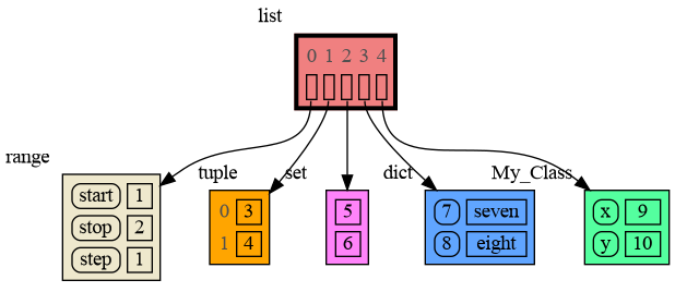
data = [ range(1, 2), (3, 4), {5, 6}, {7:'seven', 8:'eight'}, MyClass(9, 10) ]
|
|
83
|
-
|
|
83
|
+
mg.show(data, block=True)
|
|
84
84
|
```
|
|
85
85
|
|
|
86
86
|
|
|
87
|
-
By using `block=True` the program blocks until the
|
|
87
|
+
By using `block=True` the program blocks until the <Enter> key is pressed so you can view the graph before continuing program execution (and possibly viewing later graphs). Instead of showing the graph you can also render it to an output file of your choosing (see [Graphviz Output Formats](https://graphviz.org/docs/outputs/)) using for example:
|
|
88
88
|
|
|
89
89
|
```python
|
|
90
|
-
|
|
91
|
-
|
|
92
|
-
|
|
90
|
+
mg.render(data, "my_graph.pdf")
|
|
91
|
+
mg.render(data, "my_graph.png")
|
|
92
|
+
mg.render(data, "my_graph.gv") # Graphviz DOT file
|
|
93
93
|
```
|
|
94
94
|
|
|
95
95
|
# Chapters #
|
|
96
96
|
|
|
97
|
-
[
|
|
97
|
+
[Python Data Model](#python-data-model)
|
|
98
98
|
|
|
99
|
-
[
|
|
99
|
+
[Call Stack](#call-stack)
|
|
100
100
|
|
|
101
|
-
[
|
|
101
|
+
[Debugging](#Debugging)
|
|
102
102
|
|
|
103
|
-
[
|
|
103
|
+
[Datastructure Examples](#datastructure-examples)
|
|
104
104
|
|
|
105
|
-
[
|
|
105
|
+
[Configuration](#configuration)
|
|
106
106
|
|
|
107
|
-
[
|
|
107
|
+
[Extensions](#extensions)
|
|
108
108
|
|
|
109
|
-
[
|
|
109
|
+
[Jupyter Notebook](#jupyter-notebook)
|
|
110
110
|
|
|
111
|
-
[
|
|
111
|
+
[Troubleshooting](#troubleshooting)
|
|
112
112
|
|
|
113
113
|
|
|
114
114
|
## Author ##
|
|
@@ -117,27 +117,30 @@ Bas Terwijn
|
|
|
117
117
|
## Inspiration ##
|
|
118
118
|
Inspired by [Python Tutor](https://pythontutor.com/).
|
|
119
119
|
|
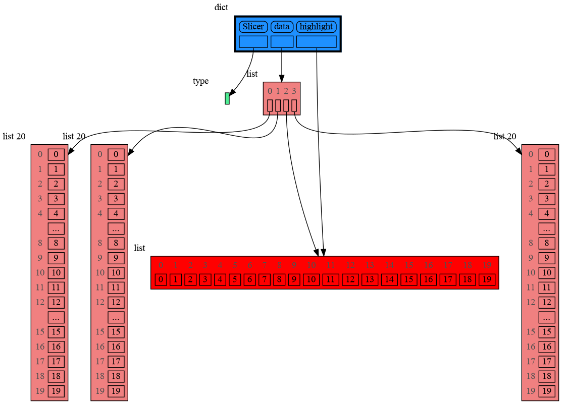
|
120
|
+
## Supported by ##
|
|
121
|
+
<img src="https://raw.githubusercontent.com/bterwijn/memory_graph/main/images/uva.png" alt="University of Amsterdam" width="600">
|
|
122
|
+
|
|
120
123
|
___
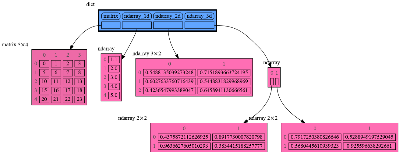
|
|
121
124
|
___
|
|
122
125
|
|
|
123
|
-
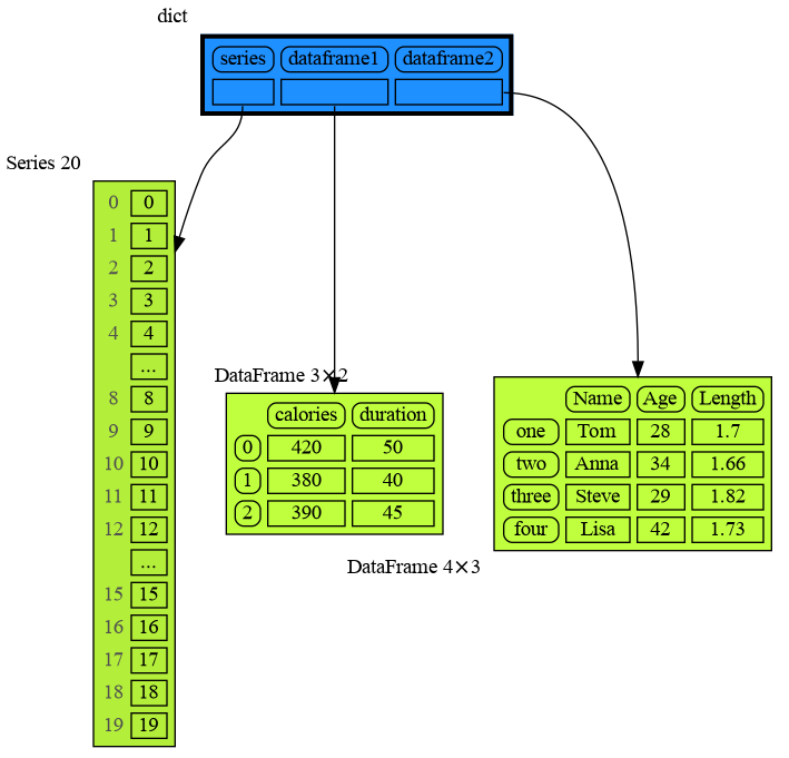
##
|
|
126
|
+
## Python Data Model ##
|
|
124
127
|
The [Python Data Model](https://docs.python.org/3/reference/datamodel.html) makes a distiction between immutable and mutable types:
|
|
125
128
|
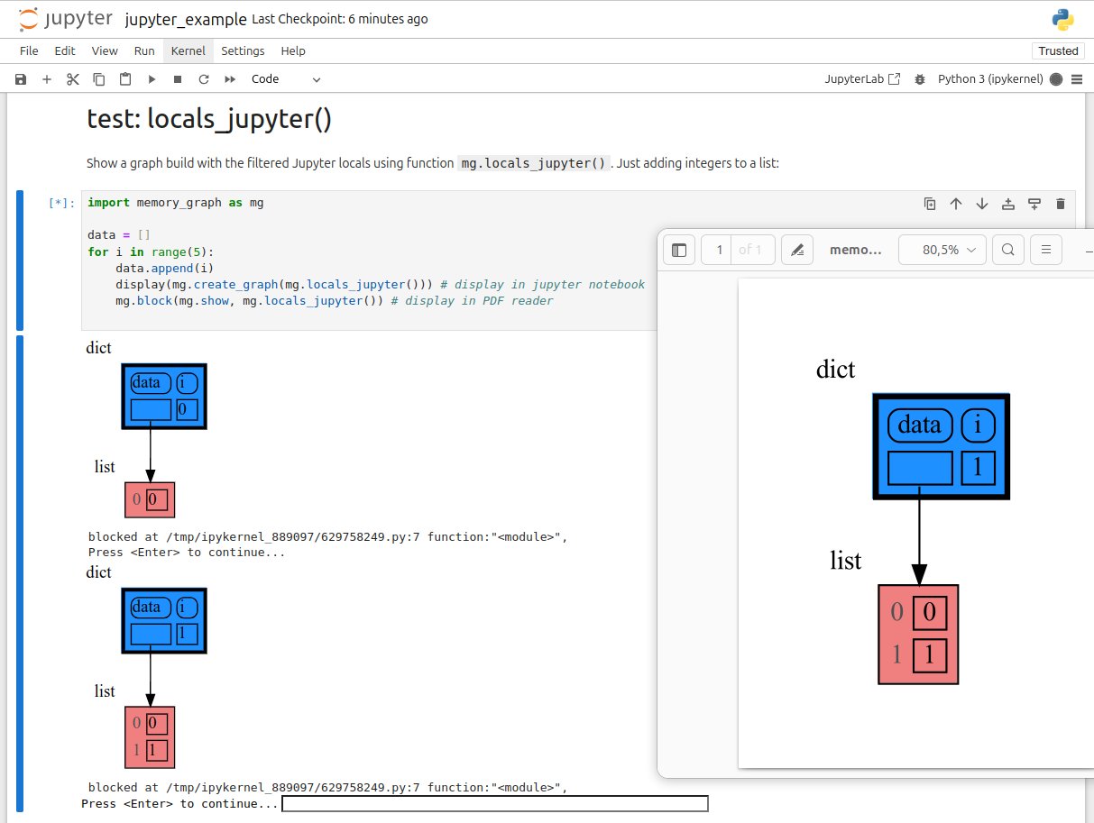
|
|
126
129
|
* **immutable**: bool, int, float, complex, str, tuple, bytes, frozenset
|
|
127
|
-
* **mutable**: list,
|
|
130
|
+
* **mutable**: list, set, dict, classes, ... (most other types)
|
|
128
131
|
|
|
129
132
|
|
|
130
133
|
### Immutable Type ###
|
|
131
|
-
In the code below variable `a` and `b` both reference the same tuple value (4, 3, 2). A tuple is an immutable type and therefore when we change variable `a` its value
|
|
134
|
+
In the code below variable `a` and `b` both reference the same tuple value (4, 3, 2). A tuple is an immutable type and therefore when we change variable `a` its value **cannot** be mutated in place, and thus a copy is made and `a` and `b` reference a different value afterwards.
|
|
132
135
|
|
|
133
136
|
```python
|
|
134
|
-
import memory_graph
|
|
137
|
+
import memory_graph as mg
|
|
135
138
|
|
|
136
139
|
a = (4, 3, 2)
|
|
137
140
|
b = a
|
|
138
|
-
|
|
141
|
+
mg.render(locals(), 'immutable1.png')
|
|
139
142
|
a += (1,)
|
|
140
|
-
|
|
143
|
+
mg.render(locals(), 'immutable2.png')
|
|
141
144
|
```
|
|
142
145
|
|  |  |
|
|
143
146
|
|:-----------------------------------------------------------:|:-------------------------------------------------------------:|
|
|
@@ -148,27 +151,25 @@ memory_graph.render(locals(), 'immutable2.png')
|
|
|
148
151
|
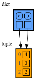
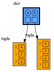
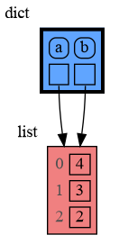
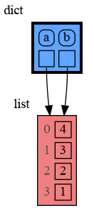
With mutable types the result is different. In the code below variable `a` and `b` both reference the same `list` value [4, 3, 2]. A `list` is a mutable type and therefore when we change variable `a` its value **can** be mutated in place and thus `a` and `b` both reference the same new value afterwards. Thus changing `a` also changes `b` and vice versa. Sometimes we want this but other times we don't and then we will have to make a copy so that `b` is independent from `a`.
|
|
149
152
|
|
|
150
153
|
```python
|
|
151
|
-
import memory_graph
|
|
154
|
+
import memory_graph as mg
|
|
152
155
|
|
|
153
156
|
a = [4, 3, 2]
|
|
154
157
|
b = a
|
|
155
|
-
|
|
158
|
+
mg.render(locals(), 'mutable1.png')
|
|
156
159
|
a += [1] # equivalent to: a.append(1)
|
|
157
|
-
|
|
160
|
+
mg.render(locals(), 'mutable2.png')
|
|
158
161
|
```
|
|
159
162
|
|  |  |
|
|
160
163
|
|:-----------------------------------------------------------:|:-------------------------------------------------------------:|
|
|
161
164
|
| mutable1.png | mutable2.png |
|
|
162
165
|
|
|
163
|
-
|
|
164
|
-
Python makes this distiction between mutable and immutable types because a value of a mutable type generally could be large and therefore it would be slow to make a copy each time we change it. On the other hand, a value of a changable immutable type generally is small and therefore fast to copy.
|
|
165
|
-
|
|
166
|
+
One practical reason why Python makes the distinction between mutable and immutable types is that a value of a mutable type could be large, making it inefficient to copy each time we change it. Immutable values generally don't need to change as much or are smaller, which makes copying less of a concern.
|
|
166
167
|
|
|
167
168
|
### Copying ###
|
|
168
169
|
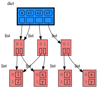
Python offers three different "copy" options that we will demonstrate using a nested list:
|
|
169
170
|
|
|
170
171
|
```python
|
|
171
|
-
import memory_graph
|
|
172
|
+
import memory_graph as mg
|
|
172
173
|
import copy
|
|
173
174
|
|
|
174
175
|
a = [ [1, 2], ['x', 'y'] ] # a nested list (a list containing lists)
|
|
@@ -178,12 +179,12 @@ c1 = a
|
|
|
178
179
|
c2 = copy.copy(a) # equivalent to: a.copy() a[:] list(a)
|
|
179
180
|
c3 = copy.deepcopy(a)
|
|
180
181
|
|
|
181
|
-
|
|
182
|
+
mg.show(locals())
|
|
182
183
|
```
|
|
183
184
|
|
|
184
|
-
* `c1` is an **assignment**, all the
|
|
185
|
-
* `c2` is a **shallow copy**, only the
|
|
186
|
-
* `c3` is a **deep copy**, all the
|
|
185
|
+
* `c1` is an **assignment**, nothing is copied, all the values are shared
|
|
186
|
+
* `c2` is a **shallow copy**, only the value referenced by the first reference is copied, all the underlying values are shared
|
|
187
|
+
* `c3` is a **deep copy**, all the values are copied, nothing is shared
|
|
187
188
|
|
|
188
189
|
|
|
189
190
|
|
|
@@ -192,7 +193,7 @@ memory_graph.show(locals())
|
|
|
192
193
|
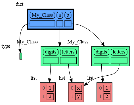
We can write our own custom copy function or method in case the three "copy" options don't do what we want. For example the copy() method of My_Class in the code below copies the `digits` but shares the `letters` between the two objects.
|
|
193
194
|
|
|
194
195
|
```python
|
|
195
|
-
import memory_graph
|
|
196
|
+
import memory_graph as mg
|
|
196
197
|
import copy
|
|
197
198
|
|
|
198
199
|
class My_Class:
|
|
@@ -209,134 +210,175 @@ class My_Class:
|
|
|
209
210
|
a = My_Class()
|
|
210
211
|
b = a.copy()
|
|
211
212
|
|
|
212
|
-
|
|
213
|
+
mg.show(locals())
|
|
213
214
|
```
|
|
214
215
|
|
|
215
216
|
|
|
216
217
|
|
|
217
|
-
##
|
|
218
|
-
|
|
219
|
-
```python
|
|
220
|
-
memory_graph.show(locals(), block=True)
|
|
221
|
-
```
|
|
218
|
+
## Call Stack ##
|
|
219
|
+
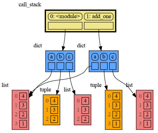
The function `mg.get_call_stack()` returns the complete call stack, including all local variables for each function in the stack. This allows us to simultaneously visualize the local variables of all the called functions. By doing so, we can identify whether any local variables from different functions in the call stack share data with one another. Here for example we call function ```add_one()``` with arguments ```a, b, c``` that adds 1 to each of its arguments.
|
|
222
220
|
|
|
223
|
-
So much so that function `d()` is available as alias for this for easier debugging. Additionally it can optionally log the data by printing them. For example:
|
|
224
221
|
```python
|
|
225
|
-
import memory_graph
|
|
226
|
-
|
|
227
|
-
squares = []
|
|
228
|
-
squares_collector = []
|
|
229
|
-
for i in range(1,6):
|
|
230
|
-
squares.append(i**2)
|
|
231
|
-
squares_collector.append(squares.copy())
|
|
232
|
-
memory_graph.d(log=True)
|
|
233
|
-
```
|
|
234
|
-
which after pressing ENTER a number of times results in:
|
|
235
|
-
|
|
236
|
-
|
|
237
|
-
```
|
|
238
|
-
squares: [1, 4, 9, 16, 25]
|
|
239
|
-
squares_collector: [[1], [1, 4], [1, 4, 9], [1, 4, 9, 16], [1, 4, 9, 16, 25]]
|
|
240
|
-
i: 5
|
|
241
|
-
```
|
|
242
|
-
|
|
243
|
-
Function `d()` has these default arguments:
|
|
244
|
-
```python
|
|
245
|
-
def d(data=None, graph=True, log=False, block=True):
|
|
246
|
-
```
|
|
247
|
-
- data: the data that is handled, defaults to `locals()` when not specified
|
|
248
|
-
- graph: if True the data is visualized as a graph
|
|
249
|
-
- log: if True the data is printed
|
|
250
|
-
- block: if True the function blocks until the ENTER key is pressed
|
|
251
|
-
|
|
252
|
-
To print to a log file instead of standard output use:
|
|
253
|
-
```python
|
|
254
|
-
memory_graph.log_file = open("my_log_file.txt", "w")
|
|
255
|
-
```
|
|
256
|
-
|
|
257
|
-
### Watchpoint in Debugger ###
|
|
258
|
-
Alternatively you get an even better debugging experience when you set expression:
|
|
259
|
-
```
|
|
260
|
-
memory_graph.render(locals(), "my_debug_graph.pdf")
|
|
261
|
-
```
|
|
262
|
-
as a *watchpoint* in a debugger tool and open the "my_debug_graph.pdf" output file. This continuouly shows the graph of all the local variables while debugging and avoids having to add any memory_graph `show()`, `render()`, or `d()` calls to your code.
|
|
263
|
-
|
|
264
|
-
|
|
265
|
-
## 3. Call Stack ##
|
|
266
|
-
The function `memory_graph.get_call_stack()` returns the complete call stack, including all local variables for each function in the stack. This allows us to simultaneously visualize the local variables of all the called functions. By doing so, we can identify whether any local variables from different functions in the call stack share data with one another. Here for example we call function ```add_one()``` with arguments ```a, b, c``` that adds 1 to each of its arguments.
|
|
267
|
-
|
|
268
|
-
```python
|
|
269
|
-
import memory_graph
|
|
222
|
+
import memory_graph as mg
|
|
270
223
|
|
|
271
224
|
def add_one(a, b, c):
|
|
272
|
-
a +=
|
|
273
|
-
b +=
|
|
225
|
+
a += [1]
|
|
226
|
+
b += (1,)
|
|
274
227
|
c += [1]
|
|
275
|
-
|
|
228
|
+
mg.show(mg.get_call_stack())
|
|
276
229
|
|
|
277
|
-
a =
|
|
278
|
-
b =
|
|
230
|
+
a = [4, 3, 2]
|
|
231
|
+
b = (4, 3, 2)
|
|
279
232
|
c = [4, 3, 2]
|
|
280
233
|
|
|
281
|
-
add_one(a, b.copy()
|
|
234
|
+
add_one(a, b, c.copy())
|
|
282
235
|
print(f"a:{a} b:{b} c:{c}")
|
|
283
236
|
```
|
|
284
237
|
|
|
285
238
|
|
|
286
|
-
In the printed output only `
|
|
239
|
+
In the printed output only `a` is changed as a result of the function call:
|
|
287
240
|
```
|
|
288
|
-
a:
|
|
241
|
+
a:[4, 3, 2, 1] b:(4, 3, 2) c:[4, 3, 2]
|
|
289
242
|
```
|
|
290
243
|
|
|
291
|
-
This is because `
|
|
244
|
+
This is because `b` is of immutable type 'tuple' so its value gets copied automatically when it is changed. And because the function is called with a copy of `c`, its original value is not changed by the function. The value of variable `a` is the only value of mutable type that is shared between the root stack frame **'0: \<module>'** and the **'1: add_one'** stack frame of the function so only that variable is affected as a result of the function call. The other changes remain confined to the local variables of the ```add_one()``` function.
|
|
292
245
|
|
|
293
246
|
|
|
294
247
|
### Recursion ###
|
|
295
248
|
The call stack can be used to visualize how recursion works. Here we show each step of how recursively ```factorial(3)``` is computed:
|
|
296
249
|
|
|
297
250
|
```python
|
|
298
|
-
import memory_graph
|
|
251
|
+
import memory_graph as mg
|
|
299
252
|
|
|
300
253
|
def factorial(n):
|
|
301
254
|
if n==0:
|
|
302
255
|
return 1
|
|
303
|
-
|
|
256
|
+
mg.show( mg.get_call_stack(), block=True )
|
|
304
257
|
result = n * factorial(n-1)
|
|
305
|
-
|
|
258
|
+
mg.show( mg.get_call_stack(), block=True )
|
|
306
259
|
return result
|
|
307
260
|
|
|
308
261
|
print(factorial(3))
|
|
309
262
|
```
|
|
263
|
+
|
|
264
|
+
Execution results in:
|
|
265
|
+
|
|
310
266
|
|
|
311
267
|
|
|
312
|
-
and the
|
|
268
|
+
and the result is: 1 x 2 x 3 = 6
|
|
269
|
+
|
|
270
|
+
### Power Set ###
|
|
271
|
+
A more insteresting recursive example that shows sharing of data is power_set(). A power set is the set of all subsets of a collection of values.
|
|
272
|
+
|
|
273
|
+
```python
|
|
274
|
+
import memory_graph as mg
|
|
275
|
+
|
|
276
|
+
def get_subsets(subsets, data, i, subset):
|
|
277
|
+
mg.show(mg.get_call_stack(), block=True)
|
|
278
|
+
if i == len(data):
|
|
279
|
+
subsets.append(subset.copy())
|
|
280
|
+
return
|
|
281
|
+
subset.append(data[i])
|
|
282
|
+
get_subsets(subsets, data, i+1, subset) # do include data[i]
|
|
283
|
+
subset.pop()
|
|
284
|
+
get_subsets(subsets, data, i+1, subset) # don't include data[i]
|
|
285
|
+
mg.show(mg.get_call_stack(), block=True)
|
|
313
286
|
|
|
314
|
-
|
|
315
|
-
|
|
287
|
+
def power_set(data):
|
|
288
|
+
subsets = []
|
|
289
|
+
get_subsets(subsets, data, 0, [])
|
|
290
|
+
return subsets
|
|
291
|
+
|
|
292
|
+
print( power_set(['a', 'b', 'c']) )
|
|
293
|
+
```
|
|
294
|
+
|
|
295
|
+
Execution results in:
|
|
296
|
+
|
|
297
|
+
|
|
298
|
+
```
|
|
299
|
+
[['a', 'b', 'c'], ['a', 'b'], ['a', 'c'], ['a'], ['b', 'c'], ['b'], ['c'], []]
|
|
300
|
+
```
|
|
301
|
+
|
|
302
|
+
|
|
303
|
+
## Debugging ##
|
|
304
|
+
|
|
305
|
+
For the best debugging experience with memory_graph set for example expression:
|
|
306
|
+
```
|
|
307
|
+
mg.render(locals(), "my_graph.pdf")
|
|
308
|
+
```
|
|
309
|
+
as a *watch* in a debugger tool such as the integrated debugger in Visual Studio Code. Then open the "my_graph.pdf" output file to continuously see all the local variables while debugging. This avoids having to add any memory_graph `show()`, `render()` calls to your code.
|
|
310
|
+
|
|
311
|
+
### Call Stack in Watch Context ###
|
|
312
|
+
The ```mg.get_call_stack()``` doesn't work well in *watch* context in most debuggers because debuggers introduce additional stack frames that cause problems. Use these alternative functions for various debuggers to filter out these problematic stack frames:
|
|
316
313
|
|
|
317
314
|
| debugger | function to get the call stack |
|
|
318
315
|
|:---|:---|
|
|
319
|
-
| **pdb, pudb** | `
|
|
320
|
-
| **Visual Studio Code** | `
|
|
321
|
-
| **Pycharm** | `
|
|
316
|
+
| **pdb, pudb** | `mg.get_call_stack_pdb()` |
|
|
317
|
+
| **Visual Studio Code** | `mg.get_call_stack_vscode()` |
|
|
318
|
+
| **Pycharm** | `mg.get_call_stack_pycharm()` |
|
|
322
319
|
|
|
323
320
|
#### Other Debuggers ####
|
|
324
|
-
For other debuggers, invoke this function within the
|
|
321
|
+
For other debuggers, invoke this function within the *watch* context. Then, in the "call_stack.txt" file, identify the slice of functions you wish to include in the call stack.
|
|
325
322
|
```
|
|
326
|
-
|
|
323
|
+
mg.save_call_stack("call_stack.txt")
|
|
327
324
|
```
|
|
328
|
-
and then call this function to get the desired call stack
|
|
325
|
+
Choose 'after' and 'up_to' what function you want to slice and then call this function to get the desired call stack:
|
|
329
326
|
```
|
|
330
|
-
|
|
327
|
+
mg.get_call_stack_after_up_to(after_function, up_to_function="<module>")
|
|
331
328
|
```
|
|
332
329
|
|
|
330
|
+
### Debugging without Debugger Tool ###
|
|
331
|
+
|
|
332
|
+
To make debugging without a debugger tool easier we provide these alias functions that you can add to your code where you want to view a graph:
|
|
333
|
+
|
|
334
|
+
| alias | function|
|
|
335
|
+
|:---|:---|
|
|
336
|
+
| `d()` | `mg.show(locals(), block=True)` |
|
|
337
|
+
| `ds()` | `mg.show(mg.get_call_stack(), block=True)` |
|
|
333
338
|
|
|
334
|
-
|
|
339
|
+
These functions have the following default arguments:
|
|
340
|
+
```python
|
|
341
|
+
def d(data=None, graph=True, log=False, block=True):
|
|
342
|
+
```
|
|
343
|
+
- data: defaults to locals() and mg.get_call_stack() respectively
|
|
344
|
+
- graph: if True the data is visualized as a graph
|
|
345
|
+
- log: if True the data is printed
|
|
346
|
+
- block: if True the function blocks until the <Enter> key is pressed
|
|
347
|
+
|
|
348
|
+
To print to a log file instead of standard output use:
|
|
349
|
+
```python
|
|
350
|
+
mg.log_file = open("my_log_file.txt", "w")
|
|
351
|
+
```
|
|
352
|
+
|
|
353
|
+
For example, executing this program:
|
|
354
|
+
|
|
355
|
+
```python
|
|
356
|
+
import memory_graph as mg
|
|
357
|
+
from memory_graph import d, ds
|
|
358
|
+
|
|
359
|
+
squares = []
|
|
360
|
+
squares_collector = []
|
|
361
|
+
for i in range(1, 6):
|
|
362
|
+
squares.append(i**2)
|
|
363
|
+
squares_collector.append(squares.copy())
|
|
364
|
+
d(log=True)
|
|
365
|
+
```
|
|
366
|
+
and pressing <Enter> a number of times, produces:
|
|
367
|
+
|
|
368
|
+

|
|
369
|
+
```
|
|
370
|
+
squares: [1, 4, 9, 16, 25]
|
|
371
|
+
squares_collector: [[1], [1, 4], [1, 4, 9], [1, 4, 9, 16], [1, 4, 9, 16, 25]]
|
|
372
|
+
i: 5
|
|
373
|
+
```
|
|
374
|
+
|
|
375
|
+
|
|
376
|
+
## Datastructure Examples ##
|
|
335
377
|
Module memory_graph can be very useful in a course about datastructures, some examples:
|
|
336
378
|
|
|
337
379
|
### Doubly Linked List ###
|
|
338
380
|
```python
|
|
339
|
-
import memory_graph
|
|
381
|
+
import memory_graph as mg
|
|
340
382
|
import random
|
|
341
383
|
random.seed(0) # use same random numbers each run
|
|
342
384
|
|
|
@@ -362,7 +404,7 @@ class LinkedList:
|
|
|
362
404
|
new_node.next = self.head
|
|
363
405
|
self.head.prev = new_node
|
|
364
406
|
self.head = new_node
|
|
365
|
-
|
|
407
|
+
mg.show(locals(), block=True) # <--- draw graph
|
|
366
408
|
|
|
367
409
|
linked_list = LinkedList()
|
|
368
410
|
n = 100
|
|
@@ -374,7 +416,7 @@ for i in range(n):
|
|
|
374
416
|
|
|
375
417
|
### Binary Tree ###
|
|
376
418
|
```python
|
|
377
|
-
import memory_graph
|
|
419
|
+
import memory_graph as mg
|
|
378
420
|
import random
|
|
379
421
|
random.seed(0) # use same random numbers each run
|
|
380
422
|
|
|
@@ -401,7 +443,7 @@ class BinTree:
|
|
|
401
443
|
node.larger = Node(new_value)
|
|
402
444
|
else:
|
|
403
445
|
self.add_recursive(new_value, node.larger)
|
|
404
|
-
|
|
446
|
+
mg.show(locals(), block=True) # <--- draw graph
|
|
405
447
|
|
|
406
448
|
def add(self, value):
|
|
407
449
|
if self.root is None:
|
|
@@ -419,7 +461,7 @@ for i in range(n):
|
|
|
419
461
|
|
|
420
462
|
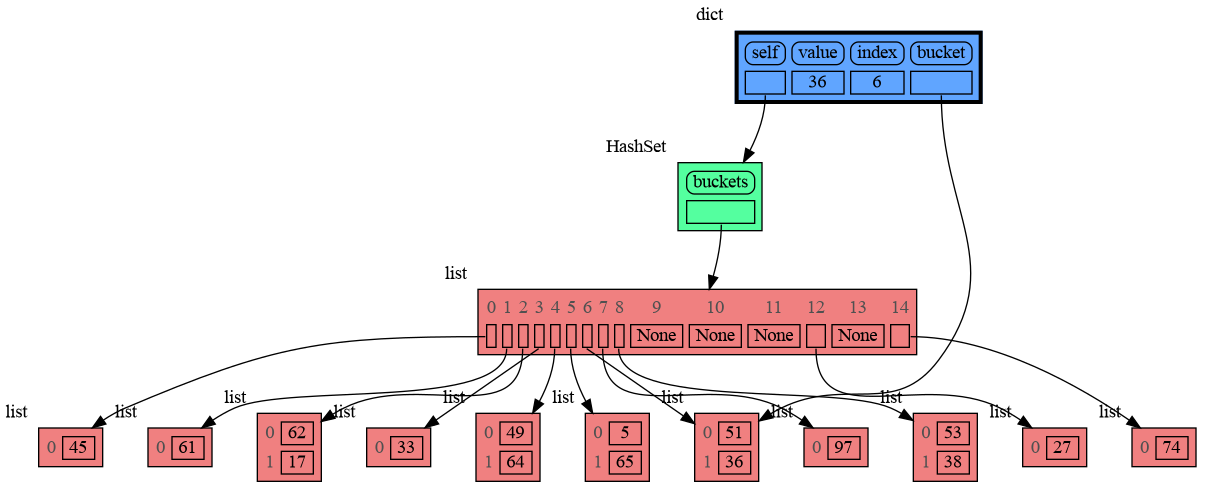
### Hash Set ###
|
|
421
463
|
```python
|
|
422
|
-
import memory_graph
|
|
464
|
+
import memory_graph as mg
|
|
423
465
|
import random
|
|
424
466
|
random.seed(0) # use same random numbers each run
|
|
425
467
|
|
|
@@ -434,7 +476,7 @@ class HashSet:
|
|
|
434
476
|
self.buckets[index] = []
|
|
435
477
|
bucket = self.buckets[index]
|
|
436
478
|
bucket.append(value)
|
|
437
|
-
|
|
479
|
+
mg.show(locals(), block=True) # <--- draw graph
|
|
438
480
|
|
|
439
481
|
def contains(self, value):
|
|
440
482
|
index = hash(value) % len(self.buckets)
|
|
@@ -456,44 +498,44 @@ for i in range(n):
|
|
|
456
498
|
|
|
457
499
|
|
|
458
500
|
|
|
459
|
-
##
|
|
460
|
-
Different aspects of memory_graph can be configured. The default configuration is reset by importing '
|
|
501
|
+
## Configuration ##
|
|
502
|
+
Different aspects of memory_graph can be configured. The default configuration is reset by importing 'mg.config_default'.
|
|
461
503
|
|
|
462
|
-
- ***
|
|
504
|
+
- ***mg.config.max_number_nodes*** : int
|
|
463
505
|
- The maxium number of Nodes shown in the graph. When the graph gets too big set this to a smaller number. A `★` symbol indictes where the graph is cut short.
|
|
464
506
|
|
|
465
|
-
- ***
|
|
507
|
+
- ***mg.config.max_string_length*** : int
|
|
466
508
|
- The maximum length of strings shown in the graph. Longer strings will be truncated.
|
|
467
509
|
|
|
468
|
-
- ***
|
|
510
|
+
- ***mg.config.not_node_types*** : set
|
|
469
511
|
- Holds all types for which no seperate node is drawn but that instead are shown as elements in their parent Node.
|
|
470
512
|
|
|
471
|
-
- ***
|
|
513
|
+
- ***mg.config.no_child_references_types*** : set
|
|
472
514
|
- The set of key_value types that don't draw references to their direct childeren but have their children shown as elements of their node.
|
|
473
515
|
|
|
474
|
-
- ***
|
|
516
|
+
- ***mg.config.type_to_node*** : dict
|
|
475
517
|
- Determines how a data types is converted to a Node (sub)class for visualization in the graph.
|
|
476
518
|
|
|
477
|
-
- ***
|
|
519
|
+
- ***mg.config.type_to_color*** : dict
|
|
478
520
|
- Maps each type to the [graphviz color](https://graphviz.org/doc/info/colors.html) it gets in the graph.
|
|
479
521
|
|
|
480
|
-
- ***
|
|
522
|
+
- ***mg.config.type_to_vertical_orientation*** : dict
|
|
481
523
|
- Maps each type to its orientation. Use 'True' for vertical and 'False' for horizontal. If not specified Node_Linear and Node_Key_Value are vertical unless they have references to children.
|
|
482
524
|
|
|
483
|
-
- ***
|
|
525
|
+
- ***mg.config.type_to_slicer*** : dict
|
|
484
526
|
- Maps each type to a Slicer. A slicer determines how many elements of a data type are shown in the graph to prevent the graph from getting too big. 'Slicer()' does no slicing, 'Slicer(1,2,3)' shows just 1 element at the beginning, 2 in the middle, and 3 at the end.
|
|
485
527
|
|
|
486
528
|
### Temporary Configuration ###
|
|
487
|
-
In addition to the global configuration, a temporary configuration can be set for a single `show()`, `render()`,
|
|
529
|
+
In addition to the global configuration, a temporary configuration can be set for a single `show()`, `render()`, `d()`, `ds()` call to change the colors, orientation, and slicer. This example highlights a particular list element in red, gives it a horizontal orientation, and overwrites the default slicer for lists:
|
|
488
530
|
|
|
489
531
|
```python
|
|
490
|
-
import memory_graph
|
|
491
|
-
from memory_graph.
|
|
532
|
+
import memory_graph as mg
|
|
533
|
+
from memory_graph.slicer import Slicer
|
|
492
534
|
|
|
493
535
|
data = [ list(range(20)) for i in range(1,5)]
|
|
494
536
|
highlight = data[2]
|
|
495
537
|
|
|
496
|
-
|
|
538
|
+
mg.show( locals(),
|
|
497
539
|
colors = {id(highlight): "red" }, # set color to "red"
|
|
498
540
|
vertical_orientations = {id(highlight): False }, # set horizontal orientation
|
|
499
541
|
slicers = {id(highlight): Slicer()} # set no slicing
|
|
@@ -501,14 +543,14 @@ memory_graph.show( locals(),
|
|
|
501
543
|
```
|
|
502
544
|
|
|
503
545
|
|
|
504
|
-
##
|
|
546
|
+
## Extensions ##
|
|
505
547
|
Different extensions are available for types from other Python packages.
|
|
506
548
|
|
|
507
549
|
### Numpy ###
|
|
508
550
|
Numpy types `arrray` and `matrix` and `ndarray` can be graphed with the "memory_graph.extension_numpy" extension:
|
|
509
551
|
|
|
510
552
|
```python
|
|
511
|
-
import memory_graph
|
|
553
|
+
import memory_graph as mg
|
|
512
554
|
import numpy as np
|
|
513
555
|
import memory_graph.extension_numpy
|
|
514
556
|
np.random.seed(0) # use same random numbers each run
|
|
@@ -516,7 +558,7 @@ np.random.seed(0) # use same random numbers each run
|
|
|
516
558
|
array = np.array([1.1, 2, 3, 4, 5])
|
|
517
559
|
matrix = np.matrix([[i*20+j for j in range(20)] for i in range(20)])
|
|
518
560
|
ndarray = np.random.rand(20,20)
|
|
519
|
-
|
|
561
|
+
mg.show(locals(), block=True)
|
|
520
562
|
```
|
|
521
563
|
|
|
522
564
|
|
|
@@ -524,7 +566,7 @@ memory_graph.d()
|
|
|
524
566
|
Pandas types `Series` and `DataFrame` can be graphed with the "memory_graph.extension_pandas" extension:
|
|
525
567
|
|
|
526
568
|
```python
|
|
527
|
-
import memory_graph
|
|
569
|
+
import memory_graph as mg
|
|
528
570
|
import pandas as pd
|
|
529
571
|
import memory_graph.extension_pandas
|
|
530
572
|
|
|
@@ -535,21 +577,20 @@ dataframe2 = pd.DataFrame({ 'Name' : [ 'Tom', 'Anna', 'Steve', 'Lisa'],
|
|
|
535
577
|
'Age' : [ 28, 34, 29, 42],
|
|
536
578
|
'Length' : [ 1.70, 1.66, 1.82, 1.73] },
|
|
537
579
|
index=['one', 'two', 'three', 'four']) # with row names
|
|
538
|
-
|
|
580
|
+
mg.show(locals(), block=True)
|
|
539
581
|
```
|
|
540
582
|
|
|
541
583
|
|
|
542
|
-
##
|
|
584
|
+
## Jupyter Notebook ##
|
|
543
585
|
|
|
544
|
-
In Jupyter Notebook `locals()` has additional variables that cause problems in the graph, use `
|
|
586
|
+
In Jupyter Notebook `locals()` has additional variables that cause problems in the graph, use `mg.locals_jupyter()` to get the local variables with these problematic variables filtered out. Use `mg.get_call_stack_jupyter()` to get the whole call stack with these variables filtered out.
|
|
545
587
|
|
|
546
588
|
See for example [jupyter_example.ipynb](https://raw.githubusercontent.com/bterwijn/memory_graph/main/images/jupyter_example.ipynb).
|
|
547
589
|
|
|
548
590
|
|
|
549
591
|
|
|
550
|
-
##
|
|
592
|
+
## Troubleshooting ##
|
|
551
593
|
|
|
552
594
|
- Adobe Acrobat Reader [doesn't refresh a PDF file](https://superuser.com/questions/337011/windows-pdf-viewer-that-auto-refreshes-pdf-when-compiling-with-pdflatex) when it changes on disk and blocks updates which results in an `Could not open 'somefile.pdf' for writing : Permission denied` error. One solution is to install a PDF reader that does refresh ([Evince](https://www.fosshub.com/Evince.html) for example) and set it as the default PDF reader. Another solution is to `render()` the graph to a different output format and open it manually.
|
|
553
595
|
|
|
554
596
|
- When graph edges overlap it can be hard to distinguish them. Using an interactive graphviz viewer, such as [xdot](https://github.com/jrfonseca/xdot.py), on a '*.gv' DOT output file will help.
|
|
555
|
-
|