mantissa-interpret 0.1.0__tar.gz
This diff represents the content of publicly available package versions that have been released to one of the supported registries. The information contained in this diff is provided for informational purposes only and reflects changes between package versions as they appear in their respective public registries.
- mantissa_interpret-0.1.0/LICENSE +21 -0
- mantissa_interpret-0.1.0/PKG-INFO +194 -0
- mantissa_interpret-0.1.0/README.md +172 -0
- mantissa_interpret-0.1.0/mantissa_interpret/__init__.py +29 -0
- mantissa_interpret-0.1.0/mantissa_interpret/gradcam.py +102 -0
- mantissa_interpret-0.1.0/mantissa_interpret/occlusion.py +81 -0
- mantissa_interpret-0.1.0/mantissa_interpret/saliency.py +65 -0
- mantissa_interpret-0.1.0/mantissa_interpret.egg-info/PKG-INFO +194 -0
- mantissa_interpret-0.1.0/mantissa_interpret.egg-info/SOURCES.txt +12 -0
- mantissa_interpret-0.1.0/mantissa_interpret.egg-info/dependency_links.txt +1 -0
- mantissa_interpret-0.1.0/mantissa_interpret.egg-info/requires.txt +11 -0
- mantissa_interpret-0.1.0/mantissa_interpret.egg-info/top_level.txt +1 -0
- mantissa_interpret-0.1.0/pyproject.toml +33 -0
- mantissa_interpret-0.1.0/setup.cfg +4 -0
|
@@ -0,0 +1,21 @@
|
|
|
1
|
+
MIT License
|
|
2
|
+
|
|
3
|
+
Copyright (c) 2026 Tekin Ertekin
|
|
4
|
+
|
|
5
|
+
Permission is hereby granted, free of charge, to any person obtaining a copy
|
|
6
|
+
of this software and associated documentation files (the "Software"), to deal
|
|
7
|
+
in the Software without restriction, including without limitation the rights
|
|
8
|
+
to use, copy, modify, merge, publish, distribute, sublicense, and/or sell
|
|
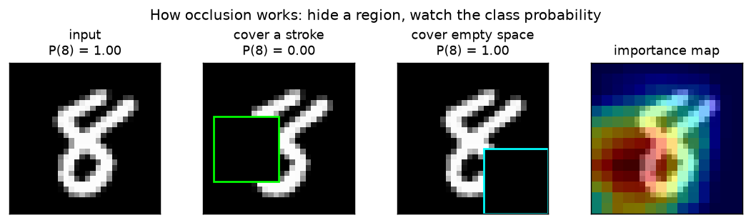
9
|
+
copies of the Software, and to permit persons to whom the Software is
|
|
10
|
+
furnished to do so, subject to the following conditions:
|
|
11
|
+
|
|
12
|
+
The above copyright notice and this permission notice shall be included in all
|
|
13
|
+
copies or substantial portions of the Software.
|
|
14
|
+
|
|
15
|
+
THE SOFTWARE IS PROVIDED "AS IS", WITHOUT WARRANTY OF ANY KIND, EXPRESS OR
|
|
16
|
+
IMPLIED, INCLUDING BUT NOT LIMITED TO THE WARRANTIES OF MERCHANTABILITY,
|
|
17
|
+
FITNESS FOR A PARTICULAR PURPOSE AND NONINFRINGEMENT. IN NO EVENT SHALL THE
|
|
18
|
+
AUTHORS OR COPYRIGHT HOLDERS BE LIABLE FOR ANY CLAIM, DAMAGES OR OTHER
|
|
19
|
+
LIABILITY, WHETHER IN AN ACTION OF CONTRACT, TORT OR OTHERWISE, ARISING FROM,
|
|
20
|
+
OUT OF OR IN CONNECTION WITH THE SOFTWARE OR THE USE OR OTHER DEALINGS IN THE
|
|
21
|
+
SOFTWARE.
|
|
@@ -0,0 +1,194 @@
|
|
|
1
|
+
Metadata-Version: 2.4
|
|
2
|
+
Name: mantissa-interpret
|
|
3
|
+
Version: 0.1.0
|
|
4
|
+
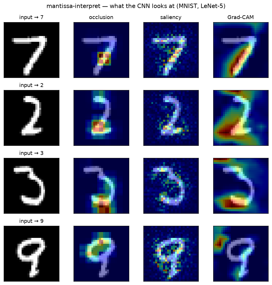
Summary: CNN interpretability on the mantissa C engine: occlusion, saliency and Grad-CAM
|
|
5
|
+
Author: Tekin Ertekin
|
|
6
|
+
License: MIT
|
|
7
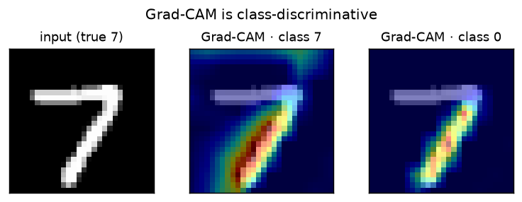
|
+
Project-URL: Homepage, https://github.com/tekinertekin/mantissa-interpret
|
|
8
|
+
Project-URL: Base, https://github.com/tekinertekin/mantissa-cnn
|
|
9
|
+
Project-URL: Engine, https://github.com/tekinertekin/mantissa
|
|
10
|
+
Requires-Python: >=3.9
|
|
11
|
+
Description-Content-Type: text/markdown
|
|
12
|
+
License-File: LICENSE
|
|
13
|
+
Requires-Dist: numpy>=1.20
|
|
14
|
+
Requires-Dist: mantissa-cnn>=0.2.2
|
|
15
|
+
Provides-Extra: viz
|
|
16
|
+
Requires-Dist: matplotlib>=3.5; extra == "viz"
|
|
17
|
+
Provides-Extra: bench
|
|
18
|
+
Requires-Dist: matplotlib>=3.5; extra == "bench"
|
|
19
|
+
Provides-Extra: dev
|
|
20
|
+
Requires-Dist: pytest>=7; extra == "dev"
|
|
21
|
+
Dynamic: license-file
|
|
22
|
+
|
|
23
|
+
# mantissa-interpret
|
|
24
|
+
|
|
25
|
+

|
|
26
|
+

|
|
27
|
+
[](https://github.com/tekinertekin/mantissa-cnn)
|
|
28
|
+
[](https://github.com/tekinertekin/mantissa)
|
|
29
|
+
|
|
30
|
+
**Seeing what a CNN looks at.** A trained classifier gives you a label; it does
|
|
31
|
+
not tell you *why*. `mantissa-interpret` answers that with three classic
|
|
32
|
+
attribution methods that turn a prediction into a **heatmap over the input** —
|
|
33
|
+
bright where the pixels mattered for the class, dark where they did not.
|
|
34
|
+
|
|
35
|
+
Everything runs on a fitted [`mantissa_cnn.Sequential`](https://github.com/tekinertekin/mantissa-cnn)
|
|
36
|
+
model, using the model's **own forward and backward passes through the mantissa
|
|
37
|
+
C engine** — the same engine it was trained on. There is no PyTorch/TensorFlow
|
|
38
|
+
dependency: the heatmaps come out of the same low-precision C kernels that
|
|
39
|
+
produced the prediction.
|
|
40
|
+
|
|
41
|
+
## The mantissa family
|
|
42
|
+
|
|
43
|
+
Part of the **mantissa** family: a low-precision engine written in C, with
|
|
44
|
+
small Python packages built on top. Each package sits under the one it depends
|
|
45
|
+
on — ⭐ marks where you are, and every other name links to its repo.
|
|
46
|
+
|
|
47
|
+
- [mantissa](https://github.com/tekinertekin/mantissa) — low-precision neural-network engine in C (the core)
|
|
48
|
+
- [mantissa-perceptron](https://github.com/tekinertekin/mantissa-perceptron) — perceptron & ADALINE, the linear classics
|
|
49
|
+
- [mantissa-nn](https://github.com/tekinertekin/mantissa-nn) — shared neural-net primitives (layers, engine binding)
|
|
50
|
+
- [mantissa-cnn](https://github.com/tekinertekin/mantissa-cnn) — convolutional networks for images
|
|
51
|
+
- [mantissa-auto-encoder](https://github.com/tekinertekin/mantissa-auto-encoder) — autoencoders for denoising & super-resolution
|
|
52
|
+
- ⭐ **mantissa-interpret** — CNN interpretability (occlusion, saliency, Grad-CAM) *(you are here)*
|
|
53
|
+
- [mantissa-embed](https://github.com/tekinertekin/mantissa-embed) — CNN metric learning (image embeddings for similarity & retrieval)
|
|
54
|
+
- [mantissa-mlp](https://github.com/tekinertekin/mantissa-mlp) — multilayer perceptrons, fully-connected nets
|
|
55
|
+
|
|
56
|
+
|
|
57
|
+
## New to interpretability?
|
|
58
|
+
|
|
59
|
+
A CNN classifier turns an image into a label — but the label alone hides *why*.
|
|
60
|
+
**Interpretability** (here, *attribution*) recovers the missing reason: it marks
|
|
61
|
+
**which parts of the input the model actually used** for a given class, as a
|
|
62
|
+
heatmap laid over the image. That matters because a model can be right for the
|
|
63
|
+
wrong reason — keying on a watermark, a background, or a dataset artifact
|
|
64
|
+
instead of the object — and a bare accuracy number will never tell you. A
|
|
65
|
+
heatmap will.
|
|
66
|
+
|
|
67
|
+
The most direct way to see this is to **hide part of the image and watch the
|
|
68
|
+
prediction**. If covering a region makes the class probability collapse, that
|
|
69
|
+
region carried the evidence; if nothing changes, it did not:
|
|
70
|
+
|
|
71
|
+
|
|
72
|
+
|
|
73
|
+
That single experiment *is* the first method. The three methods here are three
|
|
74
|
+
answers to "what did the model use?", trading detail for cost and clarity:
|
|
75
|
+
|
|
76
|
+
- **Occlusion** — exactly the picture above, done everywhere: slide a patch
|
|
77
|
+
over the image and record how much each position, when hidden, drops the
|
|
78
|
+
class probability. No math beyond running the model forward; the price is one
|
|
79
|
+
forward pass per patch, and the resolution is patch-sized.
|
|
80
|
+
- **Saliency** — instead of hiding pixels, ask calculus which pixels *matter*:
|
|
81
|
+
the gradient of the class score with respect to each input pixel. A large
|
|
82
|
+
gradient means "nudging this pixel would move the score a lot." It is
|
|
83
|
+
per-pixel sharp but noisy, and needs a single backward pass.
|
|
84
|
+
- **Grad-CAM** — work inside the network. At a convolutional layer each channel
|
|
85
|
+
is a learned feature detector over a coarse grid; weight every channel by how
|
|
86
|
+
much raising its activation would raise the target score (its gradient),
|
|
87
|
+
add them up, and keep the positive part. The result is a smooth,
|
|
88
|
+
**class-discriminative** region — ask about "3" vs "7" on the same image and
|
|
89
|
+
the map moves — for one backward pass.
|
|
90
|
+
|
|
91
|
+
Occlusion and saliency answer *which pixels*; Grad-CAM answers *which region,
|
|
92
|
+
for this class*. Together they are the standard first tools for debugging a
|
|
93
|
+
model that is right for the wrong reason.
|
|
94
|
+
|
|
95
|
+
## Install
|
|
96
|
+
|
|
97
|
+
```sh
|
|
98
|
+
pip install mantissa-interpret
|
|
99
|
+
```
|
|
100
|
+
|
|
101
|
+
Pulls in `mantissa-cnn` (and transitively `mantissa-nn` + the `mantissa-core`
|
|
102
|
+
engine). For plotting the heatmaps, `pip install mantissa-interpret[viz]`.
|
|
103
|
+
|
|
104
|
+
## The three methods
|
|
105
|
+
|
|
106
|
+
| method | cost | granularity | class-discriminative | needs |
|
|
107
|
+
|---|---|---|---|---|
|
|
108
|
+
| `occlusion_map` | forward only, O(patches) | coarse (patch) | yes | — |
|
|
109
|
+
| `saliency_map` | one backward pass | per-pixel (noisy) | weakly | input gradient |
|
|
110
|
+
| `grad_cam` | one backward pass | per-region (smooth) | **yes** | activations + their gradient at a conv layer |
|
|
111
|
+
|
|
112
|
+
Each takes a fitted model and a single `(C, H, W)` image and returns a 2-D
|
|
113
|
+
heatmap normalized to `[0, 1]`, aligned to the input.
|
|
114
|
+
|
|
115
|
+
### Occlusion — `occlusion_map`
|
|
116
|
+
|
|
117
|
+
Slide a `patch`×`patch` window (filled with `fill`) across the image; at each
|
|
118
|
+
position, hide that window and re-run the model. If the target class
|
|
119
|
+
probability drops a lot, those pixels were important. The heatmap is the
|
|
120
|
+
per-pixel average drop (overlapping windows blend), normalized to `[0, 1]`.
|
|
121
|
+
|
|
122
|
+
```python
|
|
123
|
+
from mantissa_interpret import occlusion_map
|
|
124
|
+
heat = occlusion_map(net, image, target_class=7, patch=7, stride=3)
|
|
125
|
+
```
|
|
126
|
+
|
|
127
|
+
Only forward passes — model-agnostic and dead simple, but coarse (patch-sized)
|
|
128
|
+
and its cost scales with the number of windows. All occluded copies are run in
|
|
129
|
+
a single batched forward pass.
|
|
130
|
+
|
|
131
|
+
### Saliency — `saliency_map`
|
|
132
|
+
|
|
133
|
+
The first-order sensitivity of the class score to each pixel is just its
|
|
134
|
+
gradient. One forward pass primes the layers, we seed the gradient of the
|
|
135
|
+
target *logit* (a one-hot vector), and backpropagate to the input — the same
|
|
136
|
+
`backward` the model trains with, carried one step past the first layer's
|
|
137
|
+
weights down to the pixels. The map is `|gradient|` reduced over channels.
|
|
138
|
+
|
|
139
|
+
```python
|
|
140
|
+
from mantissa_interpret import saliency_map
|
|
141
|
+
heat = saliency_map(net, image, target_class=7)
|
|
142
|
+
```
|
|
143
|
+
|
|
144
|
+
Per-pixel and cheap (one backward pass), but high-frequency and noisy, and only
|
|
145
|
+
weakly class-discriminative — good for "which strokes", not "which region".
|
|
146
|
+
|
|
147
|
+
### Grad-CAM — `grad_cam`
|
|
148
|
+
|
|
149
|
+
At a convolutional layer, each channel is a learned feature detector over a
|
|
150
|
+
coarse grid. Grad-CAM weights every channel by the average gradient of the
|
|
151
|
+
target logit w.r.t. that channel's activation (how much "more of this feature"
|
|
152
|
+
raises the class score), sums the channels with those weights, keeps the
|
|
153
|
+
positive part, and upsamples to the image. We capture the layer's activation on
|
|
154
|
+
the forward pass and backpropagate the logit down to that same layer for the
|
|
155
|
+
gradient — then combine.
|
|
156
|
+
|
|
157
|
+
```python
|
|
158
|
+
from mantissa_interpret import grad_cam
|
|
159
|
+
heat = grad_cam(net, image, target_class=7) # last Conv2D by default
|
|
160
|
+
```
|
|
161
|
+
|
|
162
|
+
Coarse (conv-grid resolution) but smooth and genuinely **class-discriminative**
|
|
163
|
+
— asking about different classes on the same image yields different maps.
|
|
164
|
+
`target_layer` selects which conv layer to read (default: the last one).
|
|
165
|
+
|
|
166
|
+
## Results
|
|
167
|
+
|
|
168
|
+
A LeNet-5 trained on an 8k-image MNIST subset with the mantissa C engine
|
|
169
|
+
(3 epochs, **96% test accuracy**), then explained on held-out digits. Reproduce
|
|
170
|
+
with `python examples/heatmaps_demo.py`.
|
|
171
|
+
|
|
172
|
+
|
|
173
|
+
|
|
174
|
+
Reading across a row, the three methods agree on the digit but differ exactly
|
|
175
|
+
as their math predicts:
|
|
176
|
+
|
|
177
|
+
- **occlusion** — coarse, patch-sized blobs on the strokes whose removal costs
|
|
178
|
+
the class the most;
|
|
179
|
+
- **saliency** — the finest detail, tracing individual strokes, but visibly
|
|
180
|
+
noisy (the raw per-pixel gradient);
|
|
181
|
+
- **Grad-CAM** — a smooth region over the class-defining strokes (the 7's
|
|
182
|
+
diagonal, the 2's base, the 9's loop), with the least clutter.
|
|
183
|
+
|
|
184
|
+
Grad-CAM is also **class-discriminative** — ask it about a different target
|
|
185
|
+
class on the *same* image and the map moves:
|
|
186
|
+
|
|
187
|
+
|
|
188
|
+
|
|
189
|
+
All of this — feature maps, gradients, the optimization-free attribution — comes
|
|
190
|
+
out of the same low-precision C kernels the model was trained on.
|
|
191
|
+
|
|
192
|
+
## License
|
|
193
|
+
|
|
194
|
+
MIT — Tekin Ertekin.
|
|
@@ -0,0 +1,172 @@
|
|
|
1
|
+
# mantissa-interpret
|
|
2
|
+
|
|
3
|
+

|
|
4
|
+

|
|
5
|
+
[](https://github.com/tekinertekin/mantissa-cnn)
|
|
6
|
+
[](https://github.com/tekinertekin/mantissa)
|
|
7
|
+
|
|
8
|
+
**Seeing what a CNN looks at.** A trained classifier gives you a label; it does
|
|
9
|
+
not tell you *why*. `mantissa-interpret` answers that with three classic
|
|
10
|
+
attribution methods that turn a prediction into a **heatmap over the input** —
|
|
11
|
+
bright where the pixels mattered for the class, dark where they did not.
|
|
12
|
+
|
|
13
|
+
Everything runs on a fitted [`mantissa_cnn.Sequential`](https://github.com/tekinertekin/mantissa-cnn)
|
|
14
|
+
model, using the model's **own forward and backward passes through the mantissa
|
|
15
|
+
C engine** — the same engine it was trained on. There is no PyTorch/TensorFlow
|
|
16
|
+
dependency: the heatmaps come out of the same low-precision C kernels that
|
|
17
|
+
produced the prediction.
|
|
18
|
+
|
|
19
|
+
## The mantissa family
|
|
20
|
+
|
|
21
|
+
Part of the **mantissa** family: a low-precision engine written in C, with
|
|
22
|
+
small Python packages built on top. Each package sits under the one it depends
|
|
23
|
+
on — ⭐ marks where you are, and every other name links to its repo.
|
|
24
|
+
|
|
25
|
+
- [mantissa](https://github.com/tekinertekin/mantissa) — low-precision neural-network engine in C (the core)
|
|
26
|
+
- [mantissa-perceptron](https://github.com/tekinertekin/mantissa-perceptron) — perceptron & ADALINE, the linear classics
|
|
27
|
+
- [mantissa-nn](https://github.com/tekinertekin/mantissa-nn) — shared neural-net primitives (layers, engine binding)
|
|
28
|
+
- [mantissa-cnn](https://github.com/tekinertekin/mantissa-cnn) — convolutional networks for images
|
|
29
|
+
- [mantissa-auto-encoder](https://github.com/tekinertekin/mantissa-auto-encoder) — autoencoders for denoising & super-resolution
|
|
30
|
+
- ⭐ **mantissa-interpret** — CNN interpretability (occlusion, saliency, Grad-CAM) *(you are here)*
|
|
31
|
+
- [mantissa-embed](https://github.com/tekinertekin/mantissa-embed) — CNN metric learning (image embeddings for similarity & retrieval)
|
|
32
|
+
- [mantissa-mlp](https://github.com/tekinertekin/mantissa-mlp) — multilayer perceptrons, fully-connected nets
|
|
33
|
+
|
|
34
|
+
|
|
35
|
+
## New to interpretability?
|
|
36
|
+
|
|
37
|
+
A CNN classifier turns an image into a label — but the label alone hides *why*.
|
|
38
|
+
**Interpretability** (here, *attribution*) recovers the missing reason: it marks
|
|
39
|
+
**which parts of the input the model actually used** for a given class, as a
|
|
40
|
+
heatmap laid over the image. That matters because a model can be right for the
|
|
41
|
+
wrong reason — keying on a watermark, a background, or a dataset artifact
|
|
42
|
+
instead of the object — and a bare accuracy number will never tell you. A
|
|
43
|
+
heatmap will.
|
|
44
|
+
|
|
45
|
+
The most direct way to see this is to **hide part of the image and watch the
|
|
46
|
+
prediction**. If covering a region makes the class probability collapse, that
|
|
47
|
+
region carried the evidence; if nothing changes, it did not:
|
|
48
|
+
|
|
49
|
+

|
|
50
|
+
|
|
51
|
+
That single experiment *is* the first method. The three methods here are three
|
|
52
|
+
answers to "what did the model use?", trading detail for cost and clarity:
|
|
53
|
+
|
|
54
|
+
- **Occlusion** — exactly the picture above, done everywhere: slide a patch
|
|
55
|
+
over the image and record how much each position, when hidden, drops the
|
|
56
|
+
class probability. No math beyond running the model forward; the price is one
|
|
57
|
+
forward pass per patch, and the resolution is patch-sized.
|
|
58
|
+
- **Saliency** — instead of hiding pixels, ask calculus which pixels *matter*:
|
|
59
|
+
the gradient of the class score with respect to each input pixel. A large
|
|
60
|
+
gradient means "nudging this pixel would move the score a lot." It is
|
|
61
|
+
per-pixel sharp but noisy, and needs a single backward pass.
|
|
62
|
+
- **Grad-CAM** — work inside the network. At a convolutional layer each channel
|
|
63
|
+
is a learned feature detector over a coarse grid; weight every channel by how
|
|
64
|
+
much raising its activation would raise the target score (its gradient),
|
|
65
|
+
add them up, and keep the positive part. The result is a smooth,
|
|
66
|
+
**class-discriminative** region — ask about "3" vs "7" on the same image and
|
|
67
|
+
the map moves — for one backward pass.
|
|
68
|
+
|
|
69
|
+
Occlusion and saliency answer *which pixels*; Grad-CAM answers *which region,
|
|
70
|
+
for this class*. Together they are the standard first tools for debugging a
|
|
71
|
+
model that is right for the wrong reason.
|
|
72
|
+
|
|
73
|
+
## Install
|
|
74
|
+
|
|
75
|
+
```sh
|
|
76
|
+
pip install mantissa-interpret
|
|
77
|
+
```
|
|
78
|
+
|
|
79
|
+
Pulls in `mantissa-cnn` (and transitively `mantissa-nn` + the `mantissa-core`
|
|
80
|
+
engine). For plotting the heatmaps, `pip install mantissa-interpret[viz]`.
|
|
81
|
+
|
|
82
|
+
## The three methods
|
|
83
|
+
|
|
84
|
+
| method | cost | granularity | class-discriminative | needs |
|
|
85
|
+
|---|---|---|---|---|
|
|
86
|
+
| `occlusion_map` | forward only, O(patches) | coarse (patch) | yes | — |
|
|
87
|
+
| `saliency_map` | one backward pass | per-pixel (noisy) | weakly | input gradient |
|
|
88
|
+
| `grad_cam` | one backward pass | per-region (smooth) | **yes** | activations + their gradient at a conv layer |
|
|
89
|
+
|
|
90
|
+
Each takes a fitted model and a single `(C, H, W)` image and returns a 2-D
|
|
91
|
+
heatmap normalized to `[0, 1]`, aligned to the input.
|
|
92
|
+
|
|
93
|
+
### Occlusion — `occlusion_map`
|
|
94
|
+
|
|
95
|
+
Slide a `patch`×`patch` window (filled with `fill`) across the image; at each
|
|
96
|
+
position, hide that window and re-run the model. If the target class
|
|
97
|
+
probability drops a lot, those pixels were important. The heatmap is the
|
|
98
|
+
per-pixel average drop (overlapping windows blend), normalized to `[0, 1]`.
|
|
99
|
+
|
|
100
|
+
```python
|
|
101
|
+
from mantissa_interpret import occlusion_map
|
|
102
|
+
heat = occlusion_map(net, image, target_class=7, patch=7, stride=3)
|
|
103
|
+
```
|
|
104
|
+
|
|
105
|
+
Only forward passes — model-agnostic and dead simple, but coarse (patch-sized)
|
|
106
|
+
and its cost scales with the number of windows. All occluded copies are run in
|
|
107
|
+
a single batched forward pass.
|
|
108
|
+
|
|
109
|
+
### Saliency — `saliency_map`
|
|
110
|
+
|
|
111
|
+
The first-order sensitivity of the class score to each pixel is just its
|
|
112
|
+
gradient. One forward pass primes the layers, we seed the gradient of the
|
|
113
|
+
target *logit* (a one-hot vector), and backpropagate to the input — the same
|
|
114
|
+
`backward` the model trains with, carried one step past the first layer's
|
|
115
|
+
weights down to the pixels. The map is `|gradient|` reduced over channels.
|
|
116
|
+
|
|
117
|
+
```python
|
|
118
|
+
from mantissa_interpret import saliency_map
|
|
119
|
+
heat = saliency_map(net, image, target_class=7)
|
|
120
|
+
```
|
|
121
|
+
|
|
122
|
+
Per-pixel and cheap (one backward pass), but high-frequency and noisy, and only
|
|
123
|
+
weakly class-discriminative — good for "which strokes", not "which region".
|
|
124
|
+
|
|
125
|
+
### Grad-CAM — `grad_cam`
|
|
126
|
+
|
|
127
|
+
At a convolutional layer, each channel is a learned feature detector over a
|
|
128
|
+
coarse grid. Grad-CAM weights every channel by the average gradient of the
|
|
129
|
+
target logit w.r.t. that channel's activation (how much "more of this feature"
|
|
130
|
+
raises the class score), sums the channels with those weights, keeps the
|
|
131
|
+
positive part, and upsamples to the image. We capture the layer's activation on
|
|
132
|
+
the forward pass and backpropagate the logit down to that same layer for the
|
|
133
|
+
gradient — then combine.
|
|
134
|
+
|
|
135
|
+
```python
|
|
136
|
+
from mantissa_interpret import grad_cam
|
|
137
|
+
heat = grad_cam(net, image, target_class=7) # last Conv2D by default
|
|
138
|
+
```
|
|
139
|
+
|
|
140
|
+
Coarse (conv-grid resolution) but smooth and genuinely **class-discriminative**
|
|
141
|
+
— asking about different classes on the same image yields different maps.
|
|
142
|
+
`target_layer` selects which conv layer to read (default: the last one).
|
|
143
|
+
|
|
144
|
+
## Results
|
|
145
|
+
|
|
146
|
+
A LeNet-5 trained on an 8k-image MNIST subset with the mantissa C engine
|
|
147
|
+
(3 epochs, **96% test accuracy**), then explained on held-out digits. Reproduce
|
|
148
|
+
with `python examples/heatmaps_demo.py`.
|
|
149
|
+
|
|
150
|
+

|
|
151
|
+
|
|
152
|
+
Reading across a row, the three methods agree on the digit but differ exactly
|
|
153
|
+
as their math predicts:
|
|
154
|
+
|
|
155
|
+
- **occlusion** — coarse, patch-sized blobs on the strokes whose removal costs
|
|
156
|
+
the class the most;
|
|
157
|
+
- **saliency** — the finest detail, tracing individual strokes, but visibly
|
|
158
|
+
noisy (the raw per-pixel gradient);
|
|
159
|
+
- **Grad-CAM** — a smooth region over the class-defining strokes (the 7's
|
|
160
|
+
diagonal, the 2's base, the 9's loop), with the least clutter.
|
|
161
|
+
|
|
162
|
+
Grad-CAM is also **class-discriminative** — ask it about a different target
|
|
163
|
+
class on the *same* image and the map moves:
|
|
164
|
+
|
|
165
|
+

|
|
166
|
+
|
|
167
|
+
All of this — feature maps, gradients, the optimization-free attribution — comes
|
|
168
|
+
out of the same low-precision C kernels the model was trained on.
|
|
169
|
+
|
|
170
|
+
## License
|
|
171
|
+
|
|
172
|
+
MIT — Tekin Ertekin.
|
|
@@ -0,0 +1,29 @@
|
|
|
1
|
+
"""mantissa-interpret: CNN interpretability on the mantissa C engine.
|
|
2
|
+
|
|
3
|
+
Attribution / visualization methods that reveal *what a trained
|
|
4
|
+
``mantissa_cnn.Sequential`` model looks at* when it makes a prediction. Each
|
|
5
|
+
method takes a fitted model and a single NCHW image and returns a 2-D heatmap
|
|
6
|
+
aligned to that image — computed with the model's own forward (and, where
|
|
7
|
+
needed, backward) passes, so it runs through the exact C engine the model was
|
|
8
|
+
trained on. No deep-learning framework is involved.
|
|
9
|
+
|
|
10
|
+
Three methods, cheapest first:
|
|
11
|
+
|
|
12
|
+
- ``occlusion_map`` — forward-only: slide a gray patch over the image and see
|
|
13
|
+
how much the target class probability drops. Model-agnostic, no gradients.
|
|
14
|
+
- ``saliency_map`` — one backward pass: |gradient of the class score w.r.t.
|
|
15
|
+
each input pixel|. Fine-grained but noisy.
|
|
16
|
+
- ``grad_cam`` — Grad-CAM: gradient-weighted activation map at a chosen
|
|
17
|
+
convolutional layer. Coarse but class-discriminative and low-noise.
|
|
18
|
+
|
|
19
|
+
>>> from mantissa_cnn import models, datasets
|
|
20
|
+
>>> from mantissa_interpret import occlusion_map, saliency_map, grad_cam
|
|
21
|
+
>>> net = models.lenet5(); net.fit(X, y, epochs=3)
|
|
22
|
+
>>> heat = grad_cam(net, image, target_class=7) # (H, W) in [0, 1]
|
|
23
|
+
"""
|
|
24
|
+
from .occlusion import occlusion_map
|
|
25
|
+
from .saliency import saliency_map
|
|
26
|
+
from .gradcam import grad_cam
|
|
27
|
+
|
|
28
|
+
__version__ = "0.1.0"
|
|
29
|
+
__all__ = ["occlusion_map", "saliency_map", "grad_cam"]
|
|
@@ -0,0 +1,102 @@
|
|
|
1
|
+
"""Grad-CAM (Selvaraju et al., 2017).
|
|
2
|
+
|
|
3
|
+
Saliency is per-pixel and noisy; Grad-CAM is per-region and class-
|
|
4
|
+
discriminative. It works at a convolutional layer, where each channel is a
|
|
5
|
+
learned feature detector over a coarse spatial grid. For a target class we
|
|
6
|
+
weight every channel by how much its activation *increasing* would raise the
|
|
7
|
+
class score (the average gradient), sum the channels with those weights, and
|
|
8
|
+
keep the positive part. The result is a coarse map of "where the evidence for
|
|
9
|
+
this class lives", which we upsample back to the image.
|
|
10
|
+
|
|
11
|
+
We reuse exactly the forward/backward the model trains with: capture the target
|
|
12
|
+
conv layer's output on the way up, backpropagate the target logit down to that
|
|
13
|
+
same layer to get its gradient, and combine.
|
|
14
|
+
"""
|
|
15
|
+
import numpy as np
|
|
16
|
+
from mantissa_cnn.layers import Conv2D
|
|
17
|
+
|
|
18
|
+
__all__ = ["grad_cam"]
|
|
19
|
+
|
|
20
|
+
|
|
21
|
+
def _bilinear(cam, out_hw):
|
|
22
|
+
"""Bilinearly resize a 2-D map to (H, W). Dependency-free."""
|
|
23
|
+
H, W = out_hw
|
|
24
|
+
h, w = cam.shape
|
|
25
|
+
if (h, w) == (H, W):
|
|
26
|
+
return cam.astype(np.float32)
|
|
27
|
+
ys = np.linspace(0.0, h - 1, H)
|
|
28
|
+
xs = np.linspace(0.0, w - 1, W)
|
|
29
|
+
y0 = np.floor(ys).astype(int); y1 = np.minimum(y0 + 1, h - 1)
|
|
30
|
+
x0 = np.floor(xs).astype(int); x1 = np.minimum(x0 + 1, w - 1)
|
|
31
|
+
wy = (ys - y0)[:, None].astype(np.float32)
|
|
32
|
+
wx = (xs - x0)[None, :].astype(np.float32)
|
|
33
|
+
top = cam[y0][:, x0] * (1 - wx) + cam[y0][:, x1] * wx
|
|
34
|
+
bot = cam[y1][:, x0] * (1 - wx) + cam[y1][:, x1] * wx
|
|
35
|
+
return (top * (1 - wy) + bot * wy).astype(np.float32)
|
|
36
|
+
|
|
37
|
+
|
|
38
|
+
def grad_cam(model, image, target_class=None, target_layer=None):
|
|
39
|
+
"""Grad-CAM heatmap for one image.
|
|
40
|
+
|
|
41
|
+
Parameters
|
|
42
|
+
----------
|
|
43
|
+
model : fitted ``mantissa_cnn.Sequential``
|
|
44
|
+
image : array (C, H, W), float32
|
|
45
|
+
target_class : int, optional
|
|
46
|
+
Class to explain. ``None`` uses the predicted class.
|
|
47
|
+
target_layer : int or Conv2D, optional
|
|
48
|
+
Which convolutional layer to read. ``None`` uses the *last* Conv2D
|
|
49
|
+
(the standard, most class-specific choice).
|
|
50
|
+
|
|
51
|
+
Returns
|
|
52
|
+
-------
|
|
53
|
+
heat : array (H, W), float32 in [0, 1]
|
|
54
|
+
"""
|
|
55
|
+
image = np.ascontiguousarray(image, dtype=np.float32)
|
|
56
|
+
if image.ndim != 3:
|
|
57
|
+
raise ValueError(f"image must be (C, H, W), got shape {image.shape}")
|
|
58
|
+
C, H, W = image.shape
|
|
59
|
+
backend = model._backend
|
|
60
|
+
layers = model.layers
|
|
61
|
+
|
|
62
|
+
if target_layer is None:
|
|
63
|
+
conv_idx = [i for i, l in enumerate(layers) if isinstance(l, Conv2D)]
|
|
64
|
+
if not conv_idx:
|
|
65
|
+
raise ValueError("model has no Conv2D layer to run Grad-CAM on")
|
|
66
|
+
target_idx = conv_idx[-1]
|
|
67
|
+
elif isinstance(target_layer, int):
|
|
68
|
+
target_idx = target_layer
|
|
69
|
+
else:
|
|
70
|
+
target_idx = layers.index(target_layer)
|
|
71
|
+
|
|
72
|
+
# Forward, copying out the target layer's activation A (the engine reuses
|
|
73
|
+
# buffers in place, so we must copy, not alias).
|
|
74
|
+
A = None
|
|
75
|
+
h = image[None]
|
|
76
|
+
for i, layer in enumerate(layers):
|
|
77
|
+
h = layer.forward(h, backend)
|
|
78
|
+
if i == target_idx:
|
|
79
|
+
A = np.array(h) # (1, K, h', w')
|
|
80
|
+
logits = h
|
|
81
|
+
|
|
82
|
+
if target_class is None:
|
|
83
|
+
target_class = int(logits[0].argmax())
|
|
84
|
+
|
|
85
|
+
dY = np.zeros_like(logits)
|
|
86
|
+
dY[0, target_class] = 1.0
|
|
87
|
+
|
|
88
|
+
# Backprop only down to the layer just above the target: the gradient
|
|
89
|
+
# handed into that layer's backward is d(logit_c)/d(A).
|
|
90
|
+
grad = dY
|
|
91
|
+
for i in range(len(layers) - 1, target_idx, -1):
|
|
92
|
+
grad = layers[i].backward(grad, backend, need_dx=True)
|
|
93
|
+
dA = np.array(grad) # (1, K, h', w')
|
|
94
|
+
|
|
95
|
+
alpha = dA.mean(axis=(2, 3)) # (1, K) channel importances
|
|
96
|
+
cam = np.maximum((alpha[:, :, None, None] * A).sum(axis=1)[0], 0.0) # (h', w')
|
|
97
|
+
|
|
98
|
+
cam = _bilinear(cam, (H, W))
|
|
99
|
+
peak = cam.max()
|
|
100
|
+
if peak > 0:
|
|
101
|
+
cam = cam / peak
|
|
102
|
+
return cam.astype(np.float32)
|
|
@@ -0,0 +1,81 @@
|
|
|
1
|
+
"""Occlusion sensitivity maps (Zeiler & Fergus, 2014).
|
|
2
|
+
|
|
3
|
+
Slide a small patch over the image, blank it out, and watch the target class
|
|
4
|
+
probability. Wherever hiding a region makes the class probability fall the
|
|
5
|
+
most, that region mattered most to the prediction. It needs nothing but the
|
|
6
|
+
model's forward pass, so it works for any classifier — no gradients, no
|
|
7
|
+
assumptions about the architecture.
|
|
8
|
+
"""
|
|
9
|
+
import numpy as np
|
|
10
|
+
|
|
11
|
+
__all__ = ["occlusion_map"]
|
|
12
|
+
|
|
13
|
+
|
|
14
|
+
def occlusion_map(model, image, target_class=None, patch=7, stride=3, fill=0.0):
|
|
15
|
+
"""Occlusion sensitivity heatmap for one image.
|
|
16
|
+
|
|
17
|
+
Parameters
|
|
18
|
+
----------
|
|
19
|
+
model : fitted ``mantissa_cnn.Sequential``
|
|
20
|
+
image : array (C, H, W), float32
|
|
21
|
+
target_class : int, optional
|
|
22
|
+
Class to explain. ``None`` uses the model's own predicted class.
|
|
23
|
+
patch : int
|
|
24
|
+
Side length of the square occluding window.
|
|
25
|
+
stride : int
|
|
26
|
+
Step between window positions (smaller = finer + slower).
|
|
27
|
+
fill : float
|
|
28
|
+
Value written into the occluded window. ``0.0`` blacks it out; the
|
|
29
|
+
image mean is a common neutral choice.
|
|
30
|
+
|
|
31
|
+
Returns
|
|
32
|
+
-------
|
|
33
|
+
heat : array (H, W), float32 in [0, 1]
|
|
34
|
+
Importance per pixel: 1 where occlusion hurt the target class most.
|
|
35
|
+
"""
|
|
36
|
+
image = np.ascontiguousarray(image, dtype=np.float32)
|
|
37
|
+
if image.ndim != 3:
|
|
38
|
+
raise ValueError(f"image must be (C, H, W), got shape {image.shape}")
|
|
39
|
+
C, H, W = image.shape
|
|
40
|
+
if patch > H or patch > W:
|
|
41
|
+
raise ValueError(f"patch {patch} larger than image {H}x{W}")
|
|
42
|
+
|
|
43
|
+
base = model.predict_proba(image[None])[0]
|
|
44
|
+
if target_class is None:
|
|
45
|
+
target_class = int(base.argmax())
|
|
46
|
+
base_p = float(base[target_class])
|
|
47
|
+
|
|
48
|
+
# Window top-left positions, always including the bottom/right edge so no
|
|
49
|
+
# border pixel is left un-probed.
|
|
50
|
+
ys = list(range(0, H - patch + 1, stride))
|
|
51
|
+
xs = list(range(0, W - patch + 1, stride))
|
|
52
|
+
if ys[-1] != H - patch:
|
|
53
|
+
ys.append(H - patch)
|
|
54
|
+
if xs[-1] != W - patch:
|
|
55
|
+
xs.append(W - patch)
|
|
56
|
+
|
|
57
|
+
# One forward pass over the whole batch of occluded copies.
|
|
58
|
+
batch = np.repeat(image[None], len(ys) * len(xs), axis=0)
|
|
59
|
+
coords = []
|
|
60
|
+
k = 0
|
|
61
|
+
for y in ys:
|
|
62
|
+
for x in xs:
|
|
63
|
+
batch[k, :, y:y + patch, x:x + patch] = fill
|
|
64
|
+
coords.append((y, x))
|
|
65
|
+
k += 1
|
|
66
|
+
probs = model.predict_proba(batch)[:, target_class]
|
|
67
|
+
drops = base_p - probs # how much hiding hurt the class
|
|
68
|
+
|
|
69
|
+
# Average each patch's drop over the pixels it covered (overlaps blend).
|
|
70
|
+
heat = np.zeros((H, W), dtype=np.float32)
|
|
71
|
+
count = np.zeros((H, W), dtype=np.float32)
|
|
72
|
+
for (y, x), d in zip(coords, drops):
|
|
73
|
+
heat[y:y + patch, x:x + patch] += d
|
|
74
|
+
count[y:y + patch, x:x + patch] += 1.0
|
|
75
|
+
heat /= np.maximum(count, 1.0)
|
|
76
|
+
|
|
77
|
+
heat = np.maximum(heat, 0.0) # keep only positive importance
|
|
78
|
+
peak = heat.max()
|
|
79
|
+
if peak > 0:
|
|
80
|
+
heat /= peak
|
|
81
|
+
return heat
|
|
@@ -0,0 +1,65 @@
|
|
|
1
|
+
"""Vanilla gradient saliency (Simonyan, Vedaldi & Zisserman, 2014).
|
|
2
|
+
|
|
3
|
+
The first-order answer to "which input pixels would change this class score
|
|
4
|
+
the most?" is simply the gradient of that score with respect to the input.
|
|
5
|
+
We run one forward pass to prime the layers, seed the gradient of the target
|
|
6
|
+
logit, and backpropagate all the way to the pixels — using the same layer
|
|
7
|
+
``backward`` passes the model trains with, only carried one step further (to
|
|
8
|
+
the input instead of stopping at the first layer's weights).
|
|
9
|
+
"""
|
|
10
|
+
import numpy as np
|
|
11
|
+
|
|
12
|
+
__all__ = ["saliency_map"]
|
|
13
|
+
|
|
14
|
+
|
|
15
|
+
def saliency_map(model, image, target_class=None):
|
|
16
|
+
"""Gradient-magnitude saliency heatmap for one image.
|
|
17
|
+
|
|
18
|
+
Parameters
|
|
19
|
+
----------
|
|
20
|
+
model : fitted ``mantissa_cnn.Sequential``
|
|
21
|
+
image : array (C, H, W), float32
|
|
22
|
+
target_class : int, optional
|
|
23
|
+
Class whose score to differentiate. ``None`` uses the predicted class.
|
|
24
|
+
|
|
25
|
+
Returns
|
|
26
|
+
-------
|
|
27
|
+
heat : array (H, W), float32 in [0, 1]
|
|
28
|
+
Per-pixel ``|d score_c / d pixel|``, reduced over channels by max.
|
|
29
|
+
|
|
30
|
+
Notes
|
|
31
|
+
-----
|
|
32
|
+
Differentiates the raw class *logit* (pre-softmax), the standard choice:
|
|
33
|
+
it isolates evidence for the class without the softmax coupling every class
|
|
34
|
+
into the gradient.
|
|
35
|
+
"""
|
|
36
|
+
image = np.ascontiguousarray(image, dtype=np.float32)
|
|
37
|
+
if image.ndim != 3:
|
|
38
|
+
raise ValueError(f"image must be (C, H, W), got shape {image.shape}")
|
|
39
|
+
backend = model._backend
|
|
40
|
+
|
|
41
|
+
# Forward pass: each layer caches what its backward needs.
|
|
42
|
+
h = image[None]
|
|
43
|
+
for layer in model.layers:
|
|
44
|
+
h = layer.forward(h, backend)
|
|
45
|
+
logits = h # (1, n_classes)
|
|
46
|
+
|
|
47
|
+
if target_class is None:
|
|
48
|
+
target_class = int(logits[0].argmax())
|
|
49
|
+
|
|
50
|
+
# Seed: d(logit_c) / d(logits) is the one-hot vector for c.
|
|
51
|
+
dY = np.zeros_like(logits)
|
|
52
|
+
dY[0, target_class] = 1.0
|
|
53
|
+
|
|
54
|
+
# Backprop to the input. need_dx=True on every layer (including the first,
|
|
55
|
+
# unlike training which stops at layer 0) so we get d(logit_c)/d(input).
|
|
56
|
+
grad = dY
|
|
57
|
+
for layer in reversed(model.layers):
|
|
58
|
+
grad = layer.backward(grad, backend, need_dx=True)
|
|
59
|
+
grad = np.asarray(grad)[0] # (C, H, W)
|
|
60
|
+
|
|
61
|
+
sal = np.abs(grad).max(axis=0) # (H, W)
|
|
62
|
+
peak = sal.max()
|
|
63
|
+
if peak > 0:
|
|
64
|
+
sal = sal / peak
|
|
65
|
+
return sal.astype(np.float32)
|
|
@@ -0,0 +1,194 @@
|
|
|
1
|
+
Metadata-Version: 2.4
|
|
2
|
+
Name: mantissa-interpret
|
|
3
|
+
Version: 0.1.0
|
|
4
|
+
Summary: CNN interpretability on the mantissa C engine: occlusion, saliency and Grad-CAM
|
|
5
|
+
Author: Tekin Ertekin
|
|
6
|
+
License: MIT
|
|
7
|
+
Project-URL: Homepage, https://github.com/tekinertekin/mantissa-interpret
|
|
8
|
+
Project-URL: Base, https://github.com/tekinertekin/mantissa-cnn
|
|
9
|
+
Project-URL: Engine, https://github.com/tekinertekin/mantissa
|
|
10
|
+
Requires-Python: >=3.9
|
|
11
|
+
Description-Content-Type: text/markdown
|
|
12
|
+
License-File: LICENSE
|
|
13
|
+
Requires-Dist: numpy>=1.20
|
|
14
|
+
Requires-Dist: mantissa-cnn>=0.2.2
|
|
15
|
+
Provides-Extra: viz
|
|
16
|
+
Requires-Dist: matplotlib>=3.5; extra == "viz"
|
|
17
|
+
Provides-Extra: bench
|
|
18
|
+
Requires-Dist: matplotlib>=3.5; extra == "bench"
|
|
19
|
+
Provides-Extra: dev
|
|
20
|
+
Requires-Dist: pytest>=7; extra == "dev"
|
|
21
|
+
Dynamic: license-file
|
|
22
|
+
|
|
23
|
+
# mantissa-interpret
|
|
24
|
+
|
|
25
|
+

|
|
26
|
+

|
|
27
|
+
[](https://github.com/tekinertekin/mantissa-cnn)
|
|
28
|
+
[](https://github.com/tekinertekin/mantissa)
|
|
29
|
+
|
|
30
|
+
**Seeing what a CNN looks at.** A trained classifier gives you a label; it does
|
|
31
|
+
not tell you *why*. `mantissa-interpret` answers that with three classic
|
|
32
|
+
attribution methods that turn a prediction into a **heatmap over the input** —
|
|
33
|
+
bright where the pixels mattered for the class, dark where they did not.
|
|
34
|
+
|
|
35
|
+
Everything runs on a fitted [`mantissa_cnn.Sequential`](https://github.com/tekinertekin/mantissa-cnn)
|
|
36
|
+
model, using the model's **own forward and backward passes through the mantissa
|
|
37
|
+
C engine** — the same engine it was trained on. There is no PyTorch/TensorFlow
|
|
38
|
+
dependency: the heatmaps come out of the same low-precision C kernels that
|
|
39
|
+
produced the prediction.
|
|
40
|
+
|
|
41
|
+
## The mantissa family
|
|
42
|
+
|
|
43
|
+
Part of the **mantissa** family: a low-precision engine written in C, with
|
|
44
|
+
small Python packages built on top. Each package sits under the one it depends
|
|
45
|
+
on — ⭐ marks where you are, and every other name links to its repo.
|
|
46
|
+
|
|
47
|
+
- [mantissa](https://github.com/tekinertekin/mantissa) — low-precision neural-network engine in C (the core)
|
|
48
|
+
- [mantissa-perceptron](https://github.com/tekinertekin/mantissa-perceptron) — perceptron & ADALINE, the linear classics
|
|
49
|
+
- [mantissa-nn](https://github.com/tekinertekin/mantissa-nn) — shared neural-net primitives (layers, engine binding)
|
|
50
|
+
- [mantissa-cnn](https://github.com/tekinertekin/mantissa-cnn) — convolutional networks for images
|
|
51
|
+
- [mantissa-auto-encoder](https://github.com/tekinertekin/mantissa-auto-encoder) — autoencoders for denoising & super-resolution
|
|
52
|
+
- ⭐ **mantissa-interpret** — CNN interpretability (occlusion, saliency, Grad-CAM) *(you are here)*
|
|
53
|
+
- [mantissa-embed](https://github.com/tekinertekin/mantissa-embed) — CNN metric learning (image embeddings for similarity & retrieval)
|
|
54
|
+
- [mantissa-mlp](https://github.com/tekinertekin/mantissa-mlp) — multilayer perceptrons, fully-connected nets
|
|
55
|
+
|
|
56
|
+
|
|
57
|
+
## New to interpretability?
|
|
58
|
+
|
|
59
|
+
A CNN classifier turns an image into a label — but the label alone hides *why*.
|
|
60
|
+
**Interpretability** (here, *attribution*) recovers the missing reason: it marks
|
|
61
|
+
**which parts of the input the model actually used** for a given class, as a
|
|
62
|
+
heatmap laid over the image. That matters because a model can be right for the
|
|
63
|
+
wrong reason — keying on a watermark, a background, or a dataset artifact
|
|
64
|
+
instead of the object — and a bare accuracy number will never tell you. A
|
|
65
|
+
heatmap will.
|
|
66
|
+
|
|
67
|
+
The most direct way to see this is to **hide part of the image and watch the
|
|
68
|
+
prediction**. If covering a region makes the class probability collapse, that
|
|
69
|
+
region carried the evidence; if nothing changes, it did not:
|
|
70
|
+
|
|
71
|
+

|
|
72
|
+
|
|
73
|
+
That single experiment *is* the first method. The three methods here are three
|
|
74
|
+
answers to "what did the model use?", trading detail for cost and clarity:
|
|
75
|
+
|
|
76
|
+
- **Occlusion** — exactly the picture above, done everywhere: slide a patch
|
|
77
|
+
over the image and record how much each position, when hidden, drops the
|
|
78
|
+
class probability. No math beyond running the model forward; the price is one
|
|
79
|
+
forward pass per patch, and the resolution is patch-sized.
|
|
80
|
+
- **Saliency** — instead of hiding pixels, ask calculus which pixels *matter*:
|
|
81
|
+
the gradient of the class score with respect to each input pixel. A large
|
|
82
|
+
gradient means "nudging this pixel would move the score a lot." It is
|
|
83
|
+
per-pixel sharp but noisy, and needs a single backward pass.
|
|
84
|
+
- **Grad-CAM** — work inside the network. At a convolutional layer each channel
|
|
85
|
+
is a learned feature detector over a coarse grid; weight every channel by how
|
|
86
|
+
much raising its activation would raise the target score (its gradient),
|
|
87
|
+
add them up, and keep the positive part. The result is a smooth,
|
|
88
|
+
**class-discriminative** region — ask about "3" vs "7" on the same image and
|
|
89
|
+
the map moves — for one backward pass.
|
|
90
|
+
|
|
91
|
+
Occlusion and saliency answer *which pixels*; Grad-CAM answers *which region,
|
|
92
|
+
for this class*. Together they are the standard first tools for debugging a
|
|
93
|
+
model that is right for the wrong reason.
|
|
94
|
+
|
|
95
|
+
## Install
|
|
96
|
+
|
|
97
|
+
```sh
|
|
98
|
+
pip install mantissa-interpret
|
|
99
|
+
```
|
|
100
|
+
|
|
101
|
+
Pulls in `mantissa-cnn` (and transitively `mantissa-nn` + the `mantissa-core`
|
|
102
|
+
engine). For plotting the heatmaps, `pip install mantissa-interpret[viz]`.
|
|
103
|
+
|
|
104
|
+
## The three methods
|
|
105
|
+
|
|
106
|
+
| method | cost | granularity | class-discriminative | needs |
|
|
107
|
+
|---|---|---|---|---|
|
|
108
|
+
| `occlusion_map` | forward only, O(patches) | coarse (patch) | yes | — |
|
|
109
|
+
| `saliency_map` | one backward pass | per-pixel (noisy) | weakly | input gradient |
|
|
110
|
+
| `grad_cam` | one backward pass | per-region (smooth) | **yes** | activations + their gradient at a conv layer |
|
|
111
|
+
|
|
112
|
+
Each takes a fitted model and a single `(C, H, W)` image and returns a 2-D
|
|
113
|
+
heatmap normalized to `[0, 1]`, aligned to the input.
|
|
114
|
+
|
|
115
|
+
### Occlusion — `occlusion_map`
|
|
116
|
+
|
|
117
|
+
Slide a `patch`×`patch` window (filled with `fill`) across the image; at each
|
|
118
|
+
position, hide that window and re-run the model. If the target class
|
|
119
|
+
probability drops a lot, those pixels were important. The heatmap is the
|
|
120
|
+
per-pixel average drop (overlapping windows blend), normalized to `[0, 1]`.
|
|
121
|
+
|
|
122
|
+
```python
|
|
123
|
+
from mantissa_interpret import occlusion_map
|
|
124
|
+
heat = occlusion_map(net, image, target_class=7, patch=7, stride=3)
|
|
125
|
+
```
|
|
126
|
+
|
|
127
|
+
Only forward passes — model-agnostic and dead simple, but coarse (patch-sized)
|
|
128
|
+
and its cost scales with the number of windows. All occluded copies are run in
|
|
129
|
+
a single batched forward pass.
|
|
130
|
+
|
|
131
|
+
### Saliency — `saliency_map`
|
|
132
|
+
|
|
133
|
+
The first-order sensitivity of the class score to each pixel is just its
|
|
134
|
+
gradient. One forward pass primes the layers, we seed the gradient of the
|
|
135
|
+
target *logit* (a one-hot vector), and backpropagate to the input — the same
|
|
136
|
+
`backward` the model trains with, carried one step past the first layer's
|
|
137
|
+
weights down to the pixels. The map is `|gradient|` reduced over channels.
|
|
138
|
+
|
|
139
|
+
```python
|
|
140
|
+
from mantissa_interpret import saliency_map
|
|
141
|
+
heat = saliency_map(net, image, target_class=7)
|
|
142
|
+
```
|
|
143
|
+
|
|
144
|
+
Per-pixel and cheap (one backward pass), but high-frequency and noisy, and only
|
|
145
|
+
weakly class-discriminative — good for "which strokes", not "which region".
|
|
146
|
+
|
|
147
|
+
### Grad-CAM — `grad_cam`
|
|
148
|
+
|
|
149
|
+
At a convolutional layer, each channel is a learned feature detector over a
|
|
150
|
+
coarse grid. Grad-CAM weights every channel by the average gradient of the
|
|
151
|
+
target logit w.r.t. that channel's activation (how much "more of this feature"
|
|
152
|
+
raises the class score), sums the channels with those weights, keeps the
|
|
153
|
+
positive part, and upsamples to the image. We capture the layer's activation on
|
|
154
|
+
the forward pass and backpropagate the logit down to that same layer for the
|
|
155
|
+
gradient — then combine.
|
|
156
|
+
|
|
157
|
+
```python
|
|
158
|
+
from mantissa_interpret import grad_cam
|
|
159
|
+
heat = grad_cam(net, image, target_class=7) # last Conv2D by default
|
|
160
|
+
```
|
|
161
|
+
|
|
162
|
+
Coarse (conv-grid resolution) but smooth and genuinely **class-discriminative**
|
|
163
|
+
— asking about different classes on the same image yields different maps.
|
|
164
|
+
`target_layer` selects which conv layer to read (default: the last one).
|
|
165
|
+
|
|
166
|
+
## Results
|
|
167
|
+
|
|
168
|
+
A LeNet-5 trained on an 8k-image MNIST subset with the mantissa C engine
|
|
169
|
+
(3 epochs, **96% test accuracy**), then explained on held-out digits. Reproduce
|
|
170
|
+
with `python examples/heatmaps_demo.py`.
|
|
171
|
+
|
|
172
|
+

|
|
173
|
+
|
|
174
|
+
Reading across a row, the three methods agree on the digit but differ exactly
|
|
175
|
+
as their math predicts:
|
|
176
|
+
|
|
177
|
+
- **occlusion** — coarse, patch-sized blobs on the strokes whose removal costs
|
|
178
|
+
the class the most;
|
|
179
|
+
- **saliency** — the finest detail, tracing individual strokes, but visibly
|
|
180
|
+
noisy (the raw per-pixel gradient);
|
|
181
|
+
- **Grad-CAM** — a smooth region over the class-defining strokes (the 7's
|
|
182
|
+
diagonal, the 2's base, the 9's loop), with the least clutter.
|
|
183
|
+
|
|
184
|
+
Grad-CAM is also **class-discriminative** — ask it about a different target
|
|
185
|
+
class on the *same* image and the map moves:
|
|
186
|
+
|
|
187
|
+

|
|
188
|
+
|
|
189
|
+
All of this — feature maps, gradients, the optimization-free attribution — comes
|
|
190
|
+
out of the same low-precision C kernels the model was trained on.
|
|
191
|
+
|
|
192
|
+
## License
|
|
193
|
+
|
|
194
|
+
MIT — Tekin Ertekin.
|
|
@@ -0,0 +1,12 @@
|
|
|
1
|
+
LICENSE
|
|
2
|
+
README.md
|
|
3
|
+
pyproject.toml
|
|
4
|
+
mantissa_interpret/__init__.py
|
|
5
|
+
mantissa_interpret/gradcam.py
|
|
6
|
+
mantissa_interpret/occlusion.py
|
|
7
|
+
mantissa_interpret/saliency.py
|
|
8
|
+
mantissa_interpret.egg-info/PKG-INFO
|
|
9
|
+
mantissa_interpret.egg-info/SOURCES.txt
|
|
10
|
+
mantissa_interpret.egg-info/dependency_links.txt
|
|
11
|
+
mantissa_interpret.egg-info/requires.txt
|
|
12
|
+
mantissa_interpret.egg-info/top_level.txt
|
|
@@ -0,0 +1 @@
|
|
|
1
|
+
|
|
@@ -0,0 +1 @@
|
|
|
1
|
+
mantissa_interpret
|
|
@@ -0,0 +1,33 @@
|
|
|
1
|
+
[build-system]
|
|
2
|
+
requires = ["setuptools>=61"]
|
|
3
|
+
build-backend = "setuptools.build_meta"
|
|
4
|
+
|
|
5
|
+
[project]
|
|
6
|
+
name = "mantissa-interpret"
|
|
7
|
+
version = "0.1.0"
|
|
8
|
+
description = "CNN interpretability on the mantissa C engine: occlusion, saliency and Grad-CAM"
|
|
9
|
+
readme = "README.md"
|
|
10
|
+
requires-python = ">=3.9"
|
|
11
|
+
license = { text = "MIT" }
|
|
12
|
+
authors = [{ name = "Tekin Ertekin" }]
|
|
13
|
+
dependencies = [
|
|
14
|
+
"numpy>=1.20",
|
|
15
|
+
# Operates on a fitted mantissa_cnn.Sequential (its layers + backend), so
|
|
16
|
+
# everything runs through the same C engine the model was trained on.
|
|
17
|
+
# mantissa-cnn transitively pulls in mantissa-nn and the mantissa-core
|
|
18
|
+
# engine. For the dev layout, `pip install -e ../cnn`.
|
|
19
|
+
"mantissa-cnn>=0.2.2",
|
|
20
|
+
]
|
|
21
|
+
|
|
22
|
+
[project.optional-dependencies]
|
|
23
|
+
viz = ["matplotlib>=3.5"]
|
|
24
|
+
bench = ["matplotlib>=3.5"]
|
|
25
|
+
dev = ["pytest>=7"]
|
|
26
|
+
|
|
27
|
+
[project.urls]
|
|
28
|
+
Homepage = "https://github.com/tekinertekin/mantissa-interpret"
|
|
29
|
+
Base = "https://github.com/tekinertekin/mantissa-cnn"
|
|
30
|
+
Engine = "https://github.com/tekinertekin/mantissa"
|
|
31
|
+
|
|
32
|
+
[tool.setuptools]
|
|
33
|
+
packages = ["mantissa_interpret"]
|