ipyrowtable 0.1.1__tar.gz
This diff represents the content of publicly available package versions that have been released to one of the supported registries. The information contained in this diff is provided for informational purposes only and reflects changes between package versions as they appear in their respective public registries.
- ipyrowtable-0.1.1/.gitignore +20 -0
- ipyrowtable-0.1.1/CHANGELOG.md +19 -0
- ipyrowtable-0.1.1/CONTRIBUTING.md +112 -0
- ipyrowtable-0.1.1/LICENSE +21 -0
- ipyrowtable-0.1.1/PKG-INFO +303 -0
- ipyrowtable-0.1.1/README.md +243 -0
- ipyrowtable-0.1.1/docs/screenshot.png +0 -0
- ipyrowtable-0.1.1/examples/01_getting_started.ipynb +244 -0
- ipyrowtable-0.1.1/examples/02_plane_wall_conduction.ipynb +229 -0
- ipyrowtable-0.1.1/examples/03_extending.ipynb +348 -0
- ipyrowtable-0.1.1/examples/04_saving_inputs.ipynb +209 -0
- ipyrowtable-0.1.1/pyproject.toml +114 -0
- ipyrowtable-0.1.1/src/ipyrowtable/__init__.py +53 -0
- ipyrowtable-0.1.1/src/ipyrowtable/columns.py +265 -0
- ipyrowtable-0.1.1/src/ipyrowtable/examples/__init__.py +4 -0
- ipyrowtable-0.1.1/src/ipyrowtable/examples/conduction.py +340 -0
- ipyrowtable-0.1.1/src/ipyrowtable/figure.py +64 -0
- ipyrowtable-0.1.1/src/ipyrowtable/formatting.py +40 -0
- ipyrowtable-0.1.1/src/ipyrowtable/layout.py +16 -0
- ipyrowtable-0.1.1/src/ipyrowtable/persistence.py +160 -0
- ipyrowtable-0.1.1/src/ipyrowtable/table.py +785 -0
- ipyrowtable-0.1.1/src/ipyrowtable/units.py +71 -0
- ipyrowtable-0.1.1/tests/__init__.py +0 -0
- ipyrowtable-0.1.1/tests/conftest.py +22 -0
- ipyrowtable-0.1.1/tests/helpers.py +106 -0
- ipyrowtable-0.1.1/tests/test_columns.py +130 -0
- ipyrowtable-0.1.1/tests/test_conduction.py +164 -0
- ipyrowtable-0.1.1/tests/test_figure.py +87 -0
- ipyrowtable-0.1.1/tests/test_notebooks.py +37 -0
- ipyrowtable-0.1.1/tests/test_persistence.py +403 -0
- ipyrowtable-0.1.1/tests/test_properties.py +208 -0
- ipyrowtable-0.1.1/tests/test_results_and_errors.py +134 -0
- ipyrowtable-0.1.1/tests/test_table.py +251 -0
- ipyrowtable-0.1.1/tests/test_units_and_formatting.py +78 -0
- ipyrowtable-0.1.1/tests/test_units_toggle.py +93 -0
- ipyrowtable-0.1.1/tests/ui/__init__.py +0 -0
- ipyrowtable-0.1.1/tests/ui/test_browser.py +129 -0
|
@@ -0,0 +1,20 @@
|
|
|
1
|
+
# Python
|
|
2
|
+
__pycache__/
|
|
3
|
+
*.py[cod]
|
|
4
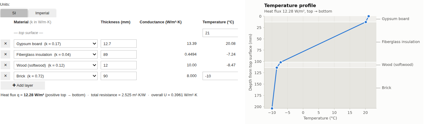
|
+
*.egg-info/
|
|
5
|
+
build/
|
|
6
|
+
dist/
|
|
7
|
+
.venv/
|
|
8
|
+
venv/
|
|
9
|
+
|
|
10
|
+
# Tools
|
|
11
|
+
.pytest_cache/
|
|
12
|
+
.hypothesis/
|
|
13
|
+
.ruff_cache/
|
|
14
|
+
.coverage
|
|
15
|
+
coverage.xml
|
|
16
|
+
htmlcov/
|
|
17
|
+
test-results/
|
|
18
|
+
|
|
19
|
+
# Jupyter
|
|
20
|
+
.ipynb_checkpoints/
|
|
@@ -0,0 +1,19 @@
|
|
|
1
|
+
# Changelog
|
|
2
|
+
|
|
3
|
+
## 0.1.1
|
|
4
|
+
|
|
5
|
+
First release.
|
|
6
|
+
|
|
7
|
+
- `RowTable`: an editable table with add and remove row buttons, live computed outputs,
|
|
8
|
+
parameters, a summary line, update callbacks, and error messages in place of results.
|
|
9
|
+
- Columns: `ChoiceColumn`, `NumberColumn`, `TextColumn`, `OutputColumn`, and `NodeColumn` for
|
|
10
|
+
values between rows with editable boundary conditions.
|
|
11
|
+
- `Unit` / `UnitSystem`, with a toggle that changes what is displayed without touching stored
|
|
12
|
+
values.
|
|
13
|
+
- `TableResults`, with base and display values and `records()`.
|
|
14
|
+
- `LiveFigure` for matplotlib plots that follow the table; `side_by_side` layout helper.
|
|
15
|
+
- `ipyrowtable.examples.conduction`: steady conduction through a plane composite wall.
|
|
16
|
+
- Saving inputs between sessions: `persist=` and `persist_file=` on `RowTable` (and
|
|
17
|
+
`LayerStack`), with a Reset button, fallback to the initial values when the saved inputs
|
|
18
|
+
can't be used, and `IPYROWTABLE_PERSIST=off` to turn saving off everywhere.
|
|
19
|
+
- `get_inputs()` / `set_inputs()` and `reset()` on `RowTable`; `validate()` on input columns.
|
|
@@ -0,0 +1,112 @@
|
|
|
1
|
+
# Contributing to ipyrowtable
|
|
2
|
+
|
|
3
|
+
## Setting up
|
|
4
|
+
|
|
5
|
+
```bash
|
|
6
|
+
git clone <your fork> && cd ipyrowtable
|
|
7
|
+
python -m venv .venv && source .venv/bin/activate # or: uv venv && source .venv/bin/activate
|
|
8
|
+
pip install -e ".[dev]"
|
|
9
|
+
```
|
|
10
|
+
|
|
11
|
+
## Tests
|
|
12
|
+
|
|
13
|
+
```bash
|
|
14
|
+
pytest # the full fast suite, about 30 s
|
|
15
|
+
pytest --cov # with a coverage report
|
|
16
|
+
pytest -m "not notebooks" # skip executing the example notebooks
|
|
17
|
+
```
|
|
18
|
+
|
|
19
|
+
The suite tests at several levels, from pure logic up to a real browser:
|
|
20
|
+
|
|
21
|
+
| Level | Files | What it checks |
|
|
22
|
+
|---|---|---|
|
|
23
|
+
| Logic | `test_units_and_formatting.py`, `test_columns.py` | unit conversions, number formatting, column widgets, header templates |
|
|
24
|
+
| Widget behavior | `test_table.py`, `test_units_toggle.py`, `test_results_and_errors.py`, `test_figure.py`, `test_persistence.py` | builds real widgets and drives them the way a user does (see below) |
|
|
25
|
+
| Invariants | `test_properties.py` | property-based tests (see below) |
|
|
26
|
+
| Physics | `test_conduction.py` | the conduction example against independent checks (see below) |
|
|
27
|
+
| Examples | `test_notebooks.py` | runs every notebook in `examples/` top to bottom in a fresh kernel |
|
|
28
|
+
| Browser | `tests/ui/` | renders the widgets in headless Chromium and uses the mouse and keyboard |
|
|
29
|
+
|
|
30
|
+
**Widget behavior.** These tests set `widget.value`, which is exactly what typing in a box
|
|
31
|
+
does, and call `button.click()`, which runs the same handlers as a mouse click. They then
|
|
32
|
+
check what the table shows and stores. No browser or kernel is needed.
|
|
33
|
+
|
|
34
|
+
**Invariants.** A hypothesis state machine plays random sequences of user actions: add and
|
|
35
|
+
remove rows, type thicknesses, pick materials, set boundaries, flip units, and start a "new
|
|
36
|
+
session" (a fresh table restoring the saved inputs). After every step it checks:
|
|
37
|
+
|
|
38
|
+
- the grid layout
|
|
39
|
+
- the stored values, against a simple model
|
|
40
|
+
- what is displayed
|
|
41
|
+
- the physics, against an independent nodal-balance solve
|
|
42
|
+
|
|
43
|
+
When a sequence fails, hypothesis shrinks it to the shortest one that still fails.
|
|
44
|
+
|
|
45
|
+
**Physics.** The conduction example is checked against things that don't share code with its
|
|
46
|
+
solver:
|
|
47
|
+
|
|
48
|
+
- Fourier's law for a single layer
|
|
49
|
+
- an independent linear-system solve
|
|
50
|
+
- symmetry when the stack is reversed
|
|
51
|
+
- NIST conversion constants
|
|
52
|
+
|
|
53
|
+
### Browser tests
|
|
54
|
+
|
|
55
|
+
`tests/ui/` uses [pytest-ipywidgets](https://solara.dev/documentation/advanced/howto/testing)
|
|
56
|
+
(from the Solara project). The widgets live in the test process, a Solara server renders
|
|
57
|
+
them with the standard ipywidgets front end, and Playwright drives headless Chromium. These
|
|
58
|
+
tests cover what the others can't: that the table renders, and that clicks and keystrokes
|
|
59
|
+
reach Python and the results come back to the page.
|
|
60
|
+
|
|
61
|
+
```bash
|
|
62
|
+
pip install -e ".[ui]"
|
|
63
|
+
playwright install chromium
|
|
64
|
+
pytest -m ui
|
|
65
|
+
```
|
|
66
|
+
|
|
67
|
+
They're excluded from the default run (`-m "not ui"` in `pyproject.toml`) because they need
|
|
68
|
+
a browser. The Solara server loads its front-end assets from cdn.jsdelivr.net, so they also
|
|
69
|
+
need network access.
|
|
70
|
+
|
|
71
|
+
### What isn't covered automatically
|
|
72
|
+
|
|
73
|
+
The browser tests render through Solara's page, not JupyterLab's. Before a release, open the
|
|
74
|
+
three notebooks in JupyterLab (and in VS Code, if you support it) and click through them.
|
|
75
|
+
Check the column alignment, the units toggle, and that the plot sits beside the table and
|
|
76
|
+
wraps below it when the window is narrow.
|
|
77
|
+
|
|
78
|
+
## Style
|
|
79
|
+
|
|
80
|
+
```bash
|
|
81
|
+
ruff check .
|
|
82
|
+
```
|
|
83
|
+
|
|
84
|
+
## Releasing
|
|
85
|
+
|
|
86
|
+
1. Update `__version__` in `src/ipyrowtable/__init__.py` and add a section to `CHANGELOG.md`.
|
|
87
|
+
2. Build and check:
|
|
88
|
+
|
|
89
|
+
```bash
|
|
90
|
+
rm -rf dist && python -m build && twine check --strict dist/*
|
|
91
|
+
```
|
|
92
|
+
|
|
93
|
+
3. Try the wheel in a clean environment:
|
|
94
|
+
|
|
95
|
+
```bash
|
|
96
|
+
python -m venv /tmp/try && /tmp/try/bin/pip install "dist/ipyrowtable-*.whl[test]"
|
|
97
|
+
cd /tmp && /tmp/try/bin/python -m pytest <repo>/tests
|
|
98
|
+
```
|
|
99
|
+
|
|
100
|
+
4. Publish:
|
|
101
|
+
- **TestPyPI first:** `twine upload --repository testpypi dist/*`, then
|
|
102
|
+
`pip install -i https://test.pypi.org/simple/ ipyrowtable` in a fresh environment.
|
|
103
|
+
- **Then PyPI**, either with `twine upload dist/*` or by publishing a GitHub release. The
|
|
104
|
+
release route runs `.github/workflows/publish.yml` using PyPI trusted publishing. To set
|
|
105
|
+
that up once, add the repository as a trusted publisher on PyPI, with workflow
|
|
106
|
+
`publish.yml` and environment `pypi`.
|
|
107
|
+
|
|
108
|
+
### Before the first release
|
|
109
|
+
|
|
110
|
+
- In `pyproject.toml`, add your name to `authors` and fill in `[project.urls]`.
|
|
111
|
+
- PyPI can't show images by relative path. Change the screenshot link in `README.md` to an
|
|
112
|
+
absolute URL, such as `https://raw.githubusercontent.com/<you>/ipyrowtable/main/docs/screenshot.png`.
|
|
@@ -0,0 +1,21 @@
|
|
|
1
|
+
MIT License
|
|
2
|
+
|
|
3
|
+
Copyright (c) 2026 The ipyrowtable authors
|
|
4
|
+
|
|
5
|
+
Permission is hereby granted, free of charge, to any person obtaining a copy
|
|
6
|
+
of this software and associated documentation files (the "Software"), to deal
|
|
7
|
+
in the Software without restriction, including without limitation the rights
|
|
8
|
+
to use, copy, modify, merge, publish, distribute, sublicense, and/or sell
|
|
9
|
+
copies of the Software, and to permit persons to whom the Software is
|
|
10
|
+
furnished to do so, subject to the following conditions:
|
|
11
|
+
|
|
12
|
+
The above copyright notice and this permission notice shall be included in all
|
|
13
|
+
copies or substantial portions of the Software.
|
|
14
|
+
|
|
15
|
+
THE SOFTWARE IS PROVIDED "AS IS", WITHOUT WARRANTY OF ANY KIND, EXPRESS OR
|
|
16
|
+
IMPLIED, INCLUDING BUT NOT LIMITED TO THE WARRANTIES OF MERCHANTABILITY,
|
|
17
|
+
FITNESS FOR A PARTICULAR PURPOSE AND NONINFRINGEMENT. IN NO EVENT SHALL THE
|
|
18
|
+
AUTHORS OR COPYRIGHT HOLDERS BE LIABLE FOR ANY CLAIM, DAMAGES OR OTHER
|
|
19
|
+
LIABILITY, WHETHER IN AN ACTION OF CONTRACT, TORT OR OTHERWISE, ARISING FROM,
|
|
20
|
+
OUT OF OR IN CONNECTION WITH THE SOFTWARE OR THE USE OR OTHER DEALINGS IN THE
|
|
21
|
+
SOFTWARE.
|
|
@@ -0,0 +1,303 @@
|
|
|
1
|
+
Metadata-Version: 2.5
|
|
2
|
+
Name: ipyrowtable
|
|
3
|
+
Version: 0.1.1
|
|
4
|
+
Summary: Editable ipywidgets tables of elements in series, with live computed columns, unit toggles and plots.
|
|
5
|
+
Author-email: jborlik@gmail.com
|
|
6
|
+
License-Expression: MIT
|
|
7
|
+
License-File: LICENSE
|
|
8
|
+
Keywords: engineering,heat transfer,ipywidgets,jupyter,table,units,widgets
|
|
9
|
+
Classifier: Development Status :: 3 - Alpha
|
|
10
|
+
Classifier: Framework :: Jupyter
|
|
11
|
+
Classifier: Framework :: Jupyter :: JupyterLab
|
|
12
|
+
Classifier: Framework :: Jupyter :: JupyterLab :: 4
|
|
13
|
+
Classifier: Intended Audience :: Education
|
|
14
|
+
Classifier: Intended Audience :: Science/Research
|
|
15
|
+
Classifier: Operating System :: OS Independent
|
|
16
|
+
Classifier: Programming Language :: Python :: 3
|
|
17
|
+
Classifier: Programming Language :: Python :: 3 :: Only
|
|
18
|
+
Classifier: Programming Language :: Python :: 3.10
|
|
19
|
+
Classifier: Programming Language :: Python :: 3.11
|
|
20
|
+
Classifier: Programming Language :: Python :: 3.12
|
|
21
|
+
Classifier: Programming Language :: Python :: 3.13
|
|
22
|
+
Classifier: Programming Language :: Python :: 3.14
|
|
23
|
+
Classifier: Topic :: Scientific/Engineering
|
|
24
|
+
Classifier: Topic :: Scientific/Engineering :: Physics
|
|
25
|
+
Requires-Python: >=3.10
|
|
26
|
+
Requires-Dist: ipywidgets>=8.1
|
|
27
|
+
Requires-Dist: numpy>=1.23
|
|
28
|
+
Provides-Extra: dev
|
|
29
|
+
Requires-Dist: build; extra == 'dev'
|
|
30
|
+
Requires-Dist: hypothesis>=6.100; extra == 'dev'
|
|
31
|
+
Requires-Dist: ipykernel>=6.29; extra == 'dev'
|
|
32
|
+
Requires-Dist: jupyterlab>=4; extra == 'dev'
|
|
33
|
+
Requires-Dist: matplotlib>=3.6; extra == 'dev'
|
|
34
|
+
Requires-Dist: nbclient>=0.10; extra == 'dev'
|
|
35
|
+
Requires-Dist: nbformat>=5.9; extra == 'dev'
|
|
36
|
+
Requires-Dist: pytest-cov>=5.0; extra == 'dev'
|
|
37
|
+
Requires-Dist: pytest>=8.0; extra == 'dev'
|
|
38
|
+
Requires-Dist: ruff; extra == 'dev'
|
|
39
|
+
Requires-Dist: twine>=6.1; extra == 'dev'
|
|
40
|
+
Provides-Extra: plot
|
|
41
|
+
Requires-Dist: matplotlib>=3.6; extra == 'plot'
|
|
42
|
+
Provides-Extra: test
|
|
43
|
+
Requires-Dist: hypothesis>=6.100; extra == 'test'
|
|
44
|
+
Requires-Dist: ipykernel>=6.29; extra == 'test'
|
|
45
|
+
Requires-Dist: matplotlib>=3.6; extra == 'test'
|
|
46
|
+
Requires-Dist: nbclient>=0.10; extra == 'test'
|
|
47
|
+
Requires-Dist: nbformat>=5.9; extra == 'test'
|
|
48
|
+
Requires-Dist: pytest-cov>=5.0; extra == 'test'
|
|
49
|
+
Requires-Dist: pytest>=8.0; extra == 'test'
|
|
50
|
+
Provides-Extra: ui
|
|
51
|
+
Requires-Dist: hypothesis>=6.100; extra == 'ui'
|
|
52
|
+
Requires-Dist: ipykernel>=6.29; extra == 'ui'
|
|
53
|
+
Requires-Dist: matplotlib>=3.6; extra == 'ui'
|
|
54
|
+
Requires-Dist: nbclient>=0.10; extra == 'ui'
|
|
55
|
+
Requires-Dist: nbformat>=5.9; extra == 'ui'
|
|
56
|
+
Requires-Dist: pytest-cov>=5.0; extra == 'ui'
|
|
57
|
+
Requires-Dist: pytest-ipywidgets>=1.40; extra == 'ui'
|
|
58
|
+
Requires-Dist: pytest>=8.0; extra == 'ui'
|
|
59
|
+
Description-Content-Type: text/markdown
|
|
60
|
+
|
|
61
|
+
# ipyrowtable
|
|
62
|
+
|
|
63
|
+
Editable [ipywidgets](https://ipywidgets.readthedocs.io) tables for problems made of elements
|
|
64
|
+
in series: wall layers, pipe segments, cable runs, process stages. You describe the columns
|
|
65
|
+
and write a `compute` function; ipyrowtable gives a table where Jupyter users add and remove
|
|
66
|
+
rows, edit inputs, see computed results update immediately, and easily use the configured inputs
|
|
67
|
+
in downstream cells.
|
|
68
|
+
|
|
69
|
+
|
|
70
|
+
|
|
71
|
+
What sets it apart from a general-purpose data grid:
|
|
72
|
+
|
|
73
|
+
- **Every cell is a real widget.** Dropdowns, number boxes and text boxes in the table itself,
|
|
74
|
+
with add and remove buttons per row.
|
|
75
|
+
- **Values between rows.** A `NodeColumn` holds the n + 1 values at the joints of n elements
|
|
76
|
+
(interface temperatures, joint pressures, node voltages), with editable boundary
|
|
77
|
+
conditions at either end.
|
|
78
|
+
- **Unit systems.** A toggle switches everything shown between, say, SI and Imperial. Values
|
|
79
|
+
are stored in your base units, so switching never changes the physics or drifts.
|
|
80
|
+
- **Live plots.** `LiveFigure` keeps a matplotlib figure in step with the table.
|
|
81
|
+
- **Saved between sessions.** A table can keep its inputs across kernel restarts, making it a
|
|
82
|
+
friendlier alternative to a hard-coded dict of inputs.
|
|
83
|
+
|
|
84
|
+
It suits small, carefully entered inputs: tens of rows, not thousands. For large data, use a
|
|
85
|
+
grid such as [ipydatagrid](https://github.com/jupyter-widgets/ipydatagrid) or Panel's
|
|
86
|
+
[Tabulator](https://panel.holoviz.org/reference/widgets/Tabulator.html).
|
|
87
|
+
|
|
88
|
+
## Install
|
|
89
|
+
|
|
90
|
+
```bash
|
|
91
|
+
pip install ipyrowtable # the table
|
|
92
|
+
pip install "ipyrowtable[plot]" # plus matplotlib, for LiveFigure and the conduction example
|
|
93
|
+
```
|
|
94
|
+
|
|
95
|
+
Needs Python 3.10+ and ipywidgets 8.1+. It uses only standard widgets, with no custom JavaScript,
|
|
96
|
+
so it works wherever ipywidgets does: JupyterLab, Jupyter Notebook, VS Code, Voilà.
|
|
97
|
+
|
|
98
|
+
## Try it
|
|
99
|
+
|
|
100
|
+
A complete application ships with the package: steady conduction through a plane composite
|
|
101
|
+
wall, with an SI / Imperial toggle and a temperature-profile plot.
|
|
102
|
+
|
|
103
|
+
```python
|
|
104
|
+
from ipyrowtable.examples.conduction import layer_stack_app
|
|
105
|
+
|
|
106
|
+
layer_stack_app(layers=[("Gypsum board", 12.7), ("Fiberglass insulation", 89), ("Brick", 90)],
|
|
107
|
+
T_top=21, T_bottom=-10)
|
|
108
|
+
```
|
|
109
|
+
|
|
110
|
+
## Quick start
|
|
111
|
+
|
|
112
|
+
Voltage along a cable run. Each row is a segment; the voltage at each joint is computed from
|
|
113
|
+
the source voltage (an editable boundary value) and the load current (a parameter that
|
|
114
|
+
applies to the whole run).
|
|
115
|
+
|
|
116
|
+
```python
|
|
117
|
+
import numpy as np
|
|
118
|
+
from ipyrowtable import ChoiceColumn, NodeColumn, NumberColumn, OutputColumn, RowTable
|
|
119
|
+
|
|
120
|
+
OHM_PER_M = {"14 AWG": 0.008286, "12 AWG": 0.005211, "10 AWG": 0.003277} # copper, 20 °C
|
|
121
|
+
|
|
122
|
+
def voltage_drop(inputs):
|
|
123
|
+
ohm_per_m = np.array([OHM_PER_M[g] for g in inputs.column("gauge")])
|
|
124
|
+
drop = 2 * inputs.params["current"] * ohm_per_m * inputs.column("length") # out and back
|
|
125
|
+
V_source = inputs.edges["voltage"][0]
|
|
126
|
+
return {"drop": drop, "voltage": V_source - np.concatenate(([0.0], np.cumsum(drop)))}
|
|
127
|
+
|
|
128
|
+
cable = RowTable(
|
|
129
|
+
columns=[
|
|
130
|
+
ChoiceColumn("gauge", "Wire", options=OHM_PER_M),
|
|
131
|
+
NumberColumn("length", "Length (m)", default=10.0, min=0),
|
|
132
|
+
OutputColumn("drop", "Drop (V)"),
|
|
133
|
+
NodeColumn("voltage", "Voltage (V)", inputs="first", first_default=120.0),
|
|
134
|
+
],
|
|
135
|
+
compute=voltage_drop,
|
|
136
|
+
parameters=[NumberColumn("current", "Current (A)", default=15.0)],
|
|
137
|
+
leading_label="— source —",
|
|
138
|
+
item_name="segment",
|
|
139
|
+
)
|
|
140
|
+
cable
|
|
141
|
+
```
|
|
142
|
+
|
|
143
|
+
`cable.results["voltage"]` holds the latest values, and `cable.results.records()` gives one
|
|
144
|
+
dict per row, ready for `pandas.DataFrame`.
|
|
145
|
+
|
|
146
|
+
## Concepts
|
|
147
|
+
|
|
148
|
+
### Columns
|
|
149
|
+
|
|
150
|
+
| Column | Kind | Per row |
|
|
151
|
+
|---|---|---|
|
|
152
|
+
| `ChoiceColumn` | input | a dropdown; options can carry data, like a material's conductivity |
|
|
153
|
+
| `NumberColumn` | input | a number, optionally unit-aware (`quantity=`) and bounded (`min=`, `max=`) |
|
|
154
|
+
| `TextColumn` | input | free text, such as a name or tag |
|
|
155
|
+
| `OutputColumn` | output | one computed value |
|
|
156
|
+
| `NodeColumn` | output | the value at the row's bottom or outlet face; the value at the top or inlet goes in a leading row |
|
|
157
|
+
|
|
158
|
+
Headers can include units: `"Thickness ({unit})"` shows the column's own unit, and
|
|
159
|
+
`"k in {conductivity}"` shows any other quantity's unit.
|
|
160
|
+
|
|
161
|
+
Input columns can also be **parameters**, shown above the table for values that apply to the
|
|
162
|
+
whole problem. To add a new input type, subclass `InputColumn` and implement `create_widget`.
|
|
163
|
+
The *03_extending* notebook adds a whole-number column this way.
|
|
164
|
+
|
|
165
|
+
### Values between rows
|
|
166
|
+
|
|
167
|
+
A `NodeColumn` holds **n + 1** values for **n** rows. Use `inputs=` to say which ends are
|
|
168
|
+
editable:
|
|
169
|
+
|
|
170
|
+
- `("first", "last")` for both ends, like the two surface temperatures of a wall
|
|
171
|
+
- `"first"` for the inlet only, like a supply pressure
|
|
172
|
+
- `"last"` for the outlet only
|
|
173
|
+
- `()` for neither
|
|
174
|
+
|
|
175
|
+
Your compute function receives the boundary values as `inputs.edges[key]` and returns all
|
|
176
|
+
n + 1 values, including the ends.
|
|
177
|
+
|
|
178
|
+
### Units
|
|
179
|
+
|
|
180
|
+
```python
|
|
181
|
+
from ipyrowtable import Unit, UnitSystem
|
|
182
|
+
|
|
183
|
+
SI = UnitSystem("SI", {"length": Unit("mm", 1000.0), "temperature": Unit("°C")})
|
|
184
|
+
IMPERIAL = UnitSystem("Imperial", {"length": Unit("in", 1 / 0.0254),
|
|
185
|
+
"temperature": Unit("°F", 1.8, 32.0)})
|
|
186
|
+
```
|
|
187
|
+
|
|
188
|
+
A `Unit` converts with `display = base × scale + offset`. Your compute function always works
|
|
189
|
+
in base units (metres and °C here). Pass `unit_systems=[SI, IMPERIAL]` to get a toggle.
|
|
190
|
+
Defaults can be given per system, such as `default={"SI": 10, "Imperial": 0.5}`, so new rows
|
|
191
|
+
start at round numbers in whichever units are showing.
|
|
192
|
+
|
|
193
|
+
### The compute function and results
|
|
194
|
+
|
|
195
|
+
`compute(inputs)` receives:
|
|
196
|
+
|
|
197
|
+
- `inputs.rows`: a list of dicts, one per row
|
|
198
|
+
- `inputs.column(key)`: one column as an array
|
|
199
|
+
- `inputs.edges`: the NodeColumn boundary values
|
|
200
|
+
- `inputs.params`: the parameters
|
|
201
|
+
|
|
202
|
+
All of them are in base units. It returns `{column key: values}`, and any extra keys (totals,
|
|
203
|
+
fluxes) are kept too. If it raises `ValueError("message")`, the message appears in place of
|
|
204
|
+
the results.
|
|
205
|
+
|
|
206
|
+
After every change:
|
|
207
|
+
|
|
208
|
+
- `table.results[key]` gives values in base units, and `table.results.display(key)` gives
|
|
209
|
+
them in the units shown.
|
|
210
|
+
- `table.results.records()` gives one dict per row.
|
|
211
|
+
- `table.on_update(callback)` runs your code with the results, or with `None` while the
|
|
212
|
+
inputs are invalid.
|
|
213
|
+
- `table.error` says what went wrong, if anything did.
|
|
214
|
+
|
|
215
|
+
### Saving inputs between sessions
|
|
216
|
+
|
|
217
|
+
```python
|
|
218
|
+
cable = RowTable(..., rows=[...], persist="feeder")
|
|
219
|
+
```
|
|
220
|
+
|
|
221
|
+
With a `persist` key, the table saves its inputs whenever they change and restores them when
|
|
222
|
+
a table with the same key is created again, for example after a kernel restart. The inputs
|
|
223
|
+
are the rows, boundary values, parameters, and the unit system that was showing.
|
|
224
|
+
|
|
225
|
+
`rows`, `edges`, `params` and `units` then become the *initial* values. They're used:
|
|
226
|
+
|
|
227
|
+
- when nothing has been saved yet;
|
|
228
|
+
- when the saved inputs can't be used, for example because an option no longer exists (the
|
|
229
|
+
table says why, and keeps the old file as a `.bak` copy before replacing it);
|
|
230
|
+
- by the **Reset** button, which asks for a second click first.
|
|
231
|
+
|
|
232
|
+
Where the inputs go:
|
|
233
|
+
|
|
234
|
+
- By default, into `<notebook name>.ipyrowtable.json` next to the notebook. If the notebook
|
|
235
|
+
can't be identified, they go into `ipyrowtable.json` in the working folder. The note under
|
|
236
|
+
the table names the file.
|
|
237
|
+
- `persist_file=` picks a different file. One file can hold many tables, each under its own
|
|
238
|
+
key.
|
|
239
|
+
- Values are stored as plain JSON in base units, so it doesn't matter which unit system was
|
|
240
|
+
showing.
|
|
241
|
+
|
|
242
|
+
They go in a file rather than the notebook's metadata because the kernel can't write
|
|
243
|
+
notebook metadata.
|
|
244
|
+
|
|
245
|
+
To always start from the initial values, leave out `persist`. The environment variable
|
|
246
|
+
`IPYROWTABLE_PERSIST=off` turns saving off for every table, which is useful for batch runs
|
|
247
|
+
that must start from known inputs. `table.get_inputs()` and `table.set_inputs(snapshot)` let
|
|
248
|
+
you keep and load snapshots yourself, such as several named designs.
|
|
249
|
+
|
|
250
|
+
### Plots
|
|
251
|
+
|
|
252
|
+
```python
|
|
253
|
+
from ipyrowtable import LiveFigure, side_by_side
|
|
254
|
+
|
|
255
|
+
def draw(fig, results):
|
|
256
|
+
ax = fig.add_subplot()
|
|
257
|
+
ax.plot(results["voltage"], marker="o")
|
|
258
|
+
|
|
259
|
+
side_by_side(cable, LiveFigure(cable, draw=draw))
|
|
260
|
+
```
|
|
261
|
+
|
|
262
|
+
### Styling
|
|
263
|
+
|
|
264
|
+
Every part carries a CSS class you can style:
|
|
265
|
+
|
|
266
|
+
- `ipyrowtable-grid`, `ipyrowtable-add`, `ipyrowtable-reset`, `ipyrowtable-message`,
|
|
267
|
+
`ipyrowtable-persist`
|
|
268
|
+
- `ipyrowtable-<key>` on each column's cells
|
|
269
|
+
|
|
270
|
+
## Examples
|
|
271
|
+
|
|
272
|
+
The [`examples/`](examples) folder has four notebooks:
|
|
273
|
+
|
|
274
|
+
1. **01_getting_started**: a first table, values between rows, a live plot, driving a table
|
|
275
|
+
from code.
|
|
276
|
+
2. **02_plane_wall_conduction**: the conduction app: units, reading results, plugging in your
|
|
277
|
+
own solver.
|
|
278
|
+
3. **03_extending**: pipes in series (Darcy–Weisbach). Covers your own unit systems, a custom
|
|
279
|
+
column type, parameters, `on_update`, and styling.
|
|
280
|
+
4. **04_saving_inputs**: keeping a table's inputs between sessions: initial values, the
|
|
281
|
+
saved file, named snapshots, resetting, and turning saving off.
|
|
282
|
+
|
|
283
|
+
## FAQ
|
|
284
|
+
|
|
285
|
+
### In VS Code, a table shows "Failed to load model class …" instead of rendering
|
|
286
|
+
|
|
287
|
+
This can happen the first time a notebook runs in VS Code's Jupyter extension, when a table is
|
|
288
|
+
created in one cell and displayed in a later one. It comes from how VS Code loads its widget
|
|
289
|
+
support: widgets created before VS Code has finished loading it can fail to render. It isn't
|
|
290
|
+
caused by ipyrowtable, which uses only standard ipywidgets. Seen with the Jupyter extension
|
|
291
|
+
2025.9.1 on Windows.
|
|
292
|
+
|
|
293
|
+
- **To fix it:** re-run the cell that creates the table, then the cell that displays it.
|
|
294
|
+
|
|
295
|
+
|
|
296
|
+
## Development
|
|
297
|
+
|
|
298
|
+
See [CONTRIBUTING.md](CONTRIBUTING.md) for setup, the test suite (including real-browser tests)
|
|
299
|
+
and releasing.
|
|
300
|
+
|
|
301
|
+
## License
|
|
302
|
+
|
|
303
|
+
MIT
|