hpspline 1.0.0__tar.gz
This diff represents the content of publicly available package versions that have been released to one of the supported registries. The information contained in this diff is provided for informational purposes only and reflects changes between package versions as they appear in their respective public registries.
- hpspline-1.0.0/LICENSE +21 -0
- hpspline-1.0.0/PKG-INFO +220 -0
- hpspline-1.0.0/README.md +198 -0
- hpspline-1.0.0/pyproject.toml +47 -0
- hpspline-1.0.0/python/hpspline.egg-info/PKG-INFO +220 -0
- hpspline-1.0.0/python/hpspline.egg-info/SOURCES.txt +9 -0
- hpspline-1.0.0/python/hpspline.egg-info/dependency_links.txt +1 -0
- hpspline-1.0.0/python/hpspline.egg-info/requires.txt +7 -0
- hpspline-1.0.0/python/hpspline.egg-info/top_level.txt +1 -0
- hpspline-1.0.0/python/hpspline.py +746 -0
- hpspline-1.0.0/setup.cfg +4 -0
hpspline-1.0.0/LICENSE
ADDED
|
@@ -0,0 +1,21 @@
|
|
|
1
|
+
MIT License
|
|
2
|
+
|
|
3
|
+
Copyright (c) 2026 Gerben van Veenendaal
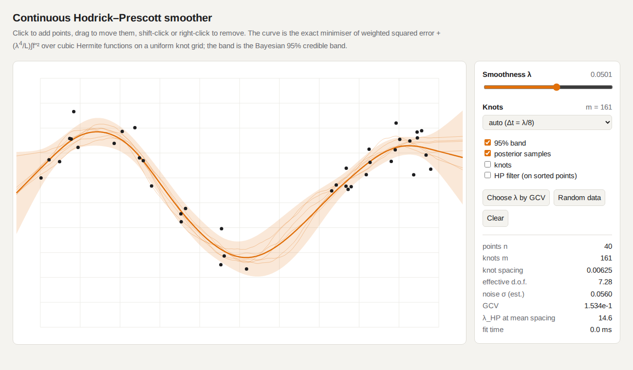
|
|
4
|
+
|
|
5
|
+
Permission is hereby granted, free of charge, to any person obtaining a copy
|
|
6
|
+
of this software and associated documentation files (the "Software"), to deal
|
|
7
|
+
in the Software without restriction, including without limitation the rights
|
|
8
|
+
to use, copy, modify, merge, publish, distribute, sublicense, and/or sell
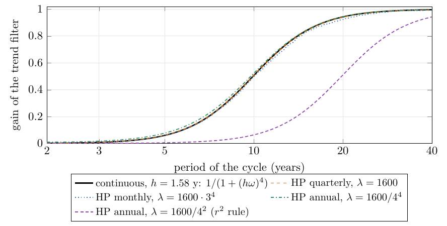
|
|
9
|
+
copies of the Software, and to permit persons to whom the Software is
|
|
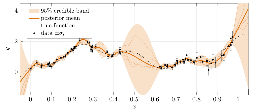
10
|
+
furnished to do so, subject to the following conditions:
|
|
11
|
+
|
|
12
|
+
The above copyright notice and this permission notice shall be included in all
|
|
13
|
+
copies or substantial portions of the Software.
|
|
14
|
+
|
|
15
|
+
THE SOFTWARE IS PROVIDED "AS IS", WITHOUT WARRANTY OF ANY KIND, EXPRESS OR
|
|
16
|
+
IMPLIED, INCLUDING BUT NOT LIMITED TO THE WARRANTIES OF MERCHANTABILITY,
|
|
17
|
+
FITNESS FOR A PARTICULAR PURPOSE AND NONINFRINGEMENT. IN NO EVENT SHALL THE
|
|
18
|
+
AUTHORS OR COPYRIGHT HOLDERS BE LIABLE FOR ANY CLAIM, DAMAGES OR OTHER
|
|
19
|
+
LIABILITY, WHETHER IN AN ACTION OF CONTRACT, TORT OR OTHERWISE, ARISING FROM,
|
|
20
|
+
OUT OF OR IN CONNECTION WITH THE SOFTWARE OR THE USE OR OTHER DEALINGS IN THE
|
|
21
|
+
SOFTWARE.
|
hpspline-1.0.0/PKG-INFO
ADDED
|
@@ -0,0 +1,220 @@
|
|
|
1
|
+
Metadata-Version: 2.4
|
|
2
|
+
Name: hpspline
|
|
3
|
+
Version: 1.0.0
|
|
4
|
+
Summary: Cubic smoothing splines on a uniform Hermite grid: a continuous Hodrick-Prescott filter with linear-time Bayesian inference
|
|
5
|
+
Author-email: Gerben van Veenendaal <gerbenvv@gmail.com>
|
|
6
|
+
License-Expression: MIT
|
|
7
|
+
Classifier: Programming Language :: Python :: 3 :: Only
|
|
8
|
+
Classifier: Programming Language :: Python :: 3.10
|
|
9
|
+
Classifier: Programming Language :: Python :: 3.11
|
|
10
|
+
Classifier: Programming Language :: Python :: 3.12
|
|
11
|
+
Classifier: Programming Language :: Python :: 3.13
|
|
12
|
+
Classifier: Programming Language :: Python :: 3.14
|
|
13
|
+
Requires-Python: >=3.10
|
|
14
|
+
Description-Content-Type: text/markdown
|
|
15
|
+
License-File: LICENSE
|
|
16
|
+
Requires-Dist: numpy
|
|
17
|
+
Provides-Extra: experiments
|
|
18
|
+
Requires-Dist: scipy; extra == "experiments"
|
|
19
|
+
Provides-Extra: fast
|
|
20
|
+
Requires-Dist: scipy; extra == "fast"
|
|
21
|
+
Dynamic: license-file
|
|
22
|
+
|
|
23
|
+
# Cubic smoothing splines on a uniform Hermite grid
|
|
24
|
+
|
|
25
|
+
**A continuous Hodrick–Prescott filter for irregular, weighted data, with linear-time Bayesian
|
|
26
|
+
inference.**
|
|
27
|
+
|
|
28
|
+
This repository contains a manuscript and two implementations (Python and JavaScript) of a smoother
|
|
29
|
+
that generalizes the Hodrick–Prescott (HP) filter to a continuous function, for data that may be
|
|
30
|
+
irregularly spaced and weighted, with exact pointwise uncertainty and a smoothing parameter measured
|
|
31
|
+
in the units of the x-axis.
|
|
32
|
+
|
|
33
|
+
- **Manuscript:** [`paper/manuscript.pdf`](paper/manuscript.pdf) (LaTeX source in
|
|
34
|
+
[`paper/`](paper/)).
|
|
35
|
+
- **Interactive demo:** try it online at <https://gerbenvv.github.io/continuous-hp-filter/>, or
|
|
36
|
+
open [`javascript/index.html`](javascript/index.html) in a browser (no server or dependencies
|
|
37
|
+
needed).
|
|
38
|
+
|
|
39
|
+
|
|
40
|
+
|
|
41
|
+
## The method
|
|
42
|
+
|
|
43
|
+
Given observations $`(x_i, y_i)`$ with weights $`w_i \ge 0`$, $`\sum_i w_i = 1`$, find the function $`f`$
|
|
44
|
+
minimizing
|
|
45
|
+
|
|
46
|
+
```math
|
|
47
|
+
J(f) = \sum_{i=1}^{n} w_i \bigl(y_i - f(x_i)\bigr)^2 + \frac{h^4}{L} \int_{t_1}^{t_m} f''(x)^2 \, dx
|
|
48
|
+
```
|
|
49
|
+
|
|
50
|
+
over $`C^1`$ piecewise cubic Hermite functions on a **uniform knot grid** $`t_1 < \dots < t_m`$ that is
|
|
51
|
+
chosen independently of the data. The unknowns are the value $`f_j`$ and derivative $`f'_j`$ at every
|
|
52
|
+
knot; $`h`$ is a bandwidth in the units of $`x`$ and $`L`$ a fixed length (the domain or data extent).
|
|
53
|
+
|
|
54
|
+
- **Exact, closed-form discretization.** Each observation adds a rank-one $`4 \times 4`$ block; the
|
|
55
|
+
roughness penalty on each element is exactly $`\theta_j^\top K \theta_j / \Delta^3`$ with the
|
|
56
|
+
Euler–Bernoulli beam stiffness matrix $`K`$.
|
|
57
|
+
- **Linear time.** The normal equations are symmetric positive definite with 7 diagonals: banded
|
|
58
|
+
Cholesky solves them in $`O(n+m)`$, and evaluation at any $`x`$ is $`O(1)`$ (no knot search on a
|
|
59
|
+
uniform grid).
|
|
60
|
+
- **Exact smoothing spline on the grid.** If every $`x_i`$ is a knot the result *is* the classical
|
|
61
|
+
(Reinsch) cubic smoothing spline; otherwise it is its best approximation in the energy norm and
|
|
62
|
+
converges to it as the grid is refined.
|
|
63
|
+
- **$`h`$ is a bandwidth.** The fit is exactly invariant under rescaling $`x`$ and $`h`$ together; for
|
|
64
|
+
evenly spread data it is a low-pass filter with gain $`1/(1+(h\omega)^4)`$ and Silverman's
|
|
65
|
+
equivalent kernel of bandwidth $`h`$.
|
|
66
|
+
- **HP is the discrete special case.** For equally spaced data the HP filter is the
|
|
67
|
+
finite-difference version of $`J`$ with $`\lambda_{\mathrm{HP}} = (h/\Delta)^4`$, which derives the
|
|
68
|
+
Ravn–Uhlig rule that $`\lambda_{\mathrm{HP}}`$ must scale with the **fourth power** of the
|
|
69
|
+
sampling frequency ($`1600 \to 1600/4^4 = 6.25`$ annual, $`1600 \cdot 3^4 = 129600`$ monthly). The
|
|
70
|
+
customary quarterly $`\lambda_{\mathrm{HP}} = 1600`$ is $`h \approx 1.58`$ years, a cutoff period of
|
|
71
|
+
about 10 years.
|
|
72
|
+
- **Bayesian uncertainty in $`O(n+m)`$.** The same matrix is the posterior precision under an
|
|
73
|
+
integrated-Wiener-process prior (exact at the knots). At every $`x`$ the posterior is Gaussian,
|
|
74
|
+
$`f(x) \mid y \sim \mathcal{N}\bigl(\varphi(x)^\top \hat\theta,\ \varphi(x)^\top A^{-1} \varphi(x) / S\bigr)`$,
|
|
75
|
+
which needs only the band of $`A^{-1}`$, computed in $`O(m)`$ by Takahashi selected inversion.
|
|
76
|
+
Posterior samples, effective degrees of freedom, a noise estimate and GCV come at the same cost.
|
|
77
|
+
|
|
78
|
+
| Frequency response of the HP filter at three sampling rates vs. the continuous filter | Irregular, heteroscedastic data with a gap: fit, 95% credible band and posterior samples |
|
|
79
|
+
| ------------------------------------------------------------------------------------------- | ----------------------------------------------------------------------------------------- |
|
|
80
|
+
|  |  |
|
|
81
|
+
|
|
82
|
+
The manuscript proves these properties, verifies each numerically, and reviews the related
|
|
83
|
+
literature (Whittaker–Henderson graduation, smoothing splines, penalized regression splines,
|
|
84
|
+
state-space and Gaussian-Markov-random-field formulations, continuous-time HP filters and
|
|
85
|
+
finite-element smoothing) with a candid assessment of what is and is not new.
|
|
86
|
+
|
|
87
|
+
## Repository layout
|
|
88
|
+
|
|
89
|
+
| Path | Contents |
|
|
90
|
+
| ----------------------------------------------- | ------------------------------------------------------------------------------------------------- |
|
|
91
|
+
| `paper/manuscript.pdf` | The manuscript |
|
|
92
|
+
| `paper/manuscript.tex`, `paper/references.bib` | LaTeX source and bibliography |
|
|
93
|
+
| `paper/data/` | Figure data and numbers used by the manuscript (generated by `python/experiments.py`) |
|
|
94
|
+
| `python/hpspline.py` | Python implementation (NumPy; uses SciPy's LAPACK banded routines when installed) |
|
|
95
|
+
| `python/tests/` | Tests against dense least squares, SciPy's exact smoothing spline, dense inverses and Monte Carlo |
|
|
96
|
+
| `python/experiments.py` | Reproduces all figures and numbers in the manuscript |
|
|
97
|
+
| `python/make_js_fixture.py` | Writes the reference results used by the JavaScript tests |
|
|
98
|
+
| `javascript/chp.js` | JavaScript implementation (browser global `CHP` or CommonJS/Node module, no dependencies) |
|
|
99
|
+
| `javascript/index.html`, `demo.js`, `style.css` | Interactive demo |
|
|
100
|
+
| `javascript/test/` | JavaScript tests against the Python reference |
|
|
101
|
+
| `docs/` | Images used in this README |
|
|
102
|
+
| `.github/workflows/pages.yml` | Publishes the interactive demo on GitHub Pages |
|
|
103
|
+
|
|
104
|
+
## Quick start
|
|
105
|
+
|
|
106
|
+
### Python
|
|
107
|
+
|
|
108
|
+
Install with `pip install hpspline` (or `pip install hpspline[fast]` to include SciPy), or
|
|
109
|
+
from a clone with `pip install .`.
|
|
110
|
+
|
|
111
|
+
```python
|
|
112
|
+
import numpy as np
|
|
113
|
+
|
|
114
|
+
from hpspline import CHPSmoother, select_lambda
|
|
115
|
+
|
|
116
|
+
x = np.sort(np.random.rand(200))
|
|
117
|
+
y = np.sin(2 * np.pi * x) + 0.1 * np.random.randn(200)
|
|
118
|
+
|
|
119
|
+
# The bandwidth `lam` is h; optionally pass `w=weights` or `sigma=known_std` to `fit`.
|
|
120
|
+
smoother = CHPSmoother(lam=0.05).fit(x, y)
|
|
121
|
+
|
|
122
|
+
# Function and derivatives, anywhere.
|
|
123
|
+
xs = np.linspace(0, 1, 1000)
|
|
124
|
+
f, df, d2f = smoother(xs), smoother(xs, nu=1), smoother(xs, nu=2)
|
|
125
|
+
|
|
126
|
+
# Posterior standard deviation (Gaussian at every x) and the 95% credible band.
|
|
127
|
+
sd = smoother.std(xs)
|
|
128
|
+
band = (f - 1.96 * sd, f + 1.96 * sd)
|
|
129
|
+
|
|
130
|
+
# Posterior samples, effective degrees of freedom, noise estimate and GCV score.
|
|
131
|
+
draws = smoother.evaluate(smoother.sample(5), xs)
|
|
132
|
+
edf, noise_variance, gcv = smoother.edf, smoother.noise_variance, smoother.gcv()
|
|
133
|
+
|
|
134
|
+
# Choose the bandwidth by GCV.
|
|
135
|
+
best, _, _ = select_lambda(x, y)
|
|
136
|
+
```
|
|
137
|
+
|
|
138
|
+
Options: `m` (number of knots) or `dt` (knot spacing; default `lam / 8`), `bounds`, and
|
|
139
|
+
`normalization` (`"domain"`, `"data"` or a number, the length $`L`$). Helpers: `hp_filter(y, lam_hp)`,
|
|
140
|
+
`lambda_from_hp(lam_hp, spacing)` and `hp_from_lambda(lam, spacing)`.
|
|
141
|
+
|
|
142
|
+
### JavaScript
|
|
143
|
+
|
|
144
|
+
```html
|
|
145
|
+
<script src="chp.js"></script>
|
|
146
|
+
<script>
|
|
147
|
+
const smoother = new CHP.CHPSmoother(0.05).fit(x, y, { w }); // Or { sigma }.
|
|
148
|
+
|
|
149
|
+
smoother.evaluate(0.3);
|
|
150
|
+
smoother.evaluate(0.3, 1);
|
|
151
|
+
smoother.std(0.3);
|
|
152
|
+
|
|
153
|
+
const theta = smoother.sample();
|
|
154
|
+
smoother.evaluateTheta(theta, 0.3);
|
|
155
|
+
|
|
156
|
+
smoother.edf();
|
|
157
|
+
smoother.noiseVariance();
|
|
158
|
+
smoother.gcv();
|
|
159
|
+
|
|
160
|
+
CHP.selectLambda(x, y).lambda;
|
|
161
|
+
</script>
|
|
162
|
+
```
|
|
163
|
+
|
|
164
|
+
In Node.js: `const CHP = require('./javascript/chp.js');`. A million observations on a million
|
|
165
|
+
knots fit in about 0.3 s.
|
|
166
|
+
|
|
167
|
+
## Development
|
|
168
|
+
|
|
169
|
+
```bash
|
|
170
|
+
# Python tests (NumPy only; the SciPy-based checks run when SciPy is installed).
|
|
171
|
+
cd python && python -m unittest discover -s tests -p "*_test.py" -t .
|
|
172
|
+
|
|
173
|
+
# JavaScript tests and formatting/linting.
|
|
174
|
+
cd javascript && npm install && npm test && npm run format
|
|
175
|
+
|
|
176
|
+
# Formatting of all files (black, isort, flake8, mdformat, eslint, ...).
|
|
177
|
+
pre-commit run -a
|
|
178
|
+
|
|
179
|
+
# Regenerate the manuscript's figures and numbers (needs SciPy and Node.js).
|
|
180
|
+
cd python && python experiments.py && python make_js_fixture.py
|
|
181
|
+
|
|
182
|
+
# Build the manuscript (TeX Live with pgfplots).
|
|
183
|
+
cd paper && pdflatex manuscript && bibtex manuscript && pdflatex manuscript && pdflatex manuscript
|
|
184
|
+
```
|
|
185
|
+
|
|
186
|
+
## Related work
|
|
187
|
+
|
|
188
|
+
The method combines well-established ideas; see Section 10 of the manuscript. The closest prior work
|
|
189
|
+
includes O'Sullivan penalized splines (O'Sullivan 1986; Wand & Ormerod 2008), finite-element
|
|
190
|
+
approximations of the integrated Wiener process on equally spaced knots (Zhang, Stringer, Brown &
|
|
191
|
+
Stafford 2024), the augmented-state second-order random walk (Rue & Held 2005; Lindgren & Rue 2008),
|
|
192
|
+
continuous-time HP filters (Iannaccone & Otranto 2003; McElroy & Trimbur 2007), the Hermite
|
|
193
|
+
value–derivative spline parametrization (Costa & Shaw 2009), and the smoothing-spline and Bayesian
|
|
194
|
+
foundations of Schoenberg, Reinsch, Wahba and Silverman.
|
|
195
|
+
|
|
196
|
+
## Citation
|
|
197
|
+
|
|
198
|
+
If you use this work (the method, the manuscript or the code), please cite it:
|
|
199
|
+
|
|
200
|
+
> Gerben van Veenendaal. *Cubic Smoothing Splines on a Uniform Hermite Grid: A Continuous
|
|
201
|
+
> Hodrick–Prescott Filter for Irregular, Weighted Data with Linear-Time Bayesian Inference.*
|
|
202
|
+
> Manuscript, 2026. https://github.com/gerbenvv/continuous-hp-filter
|
|
203
|
+
|
|
204
|
+
```bibtex
|
|
205
|
+
@unpublished{vanVeenendaal2026,
|
|
206
|
+
author = {van Veenendaal, Gerben},
|
|
207
|
+
title = {Cubic Smoothing Splines on a Uniform {H}ermite Grid: A Continuous {H}odrick--{P}rescott
|
|
208
|
+
Filter for Irregular, Weighted Data with Linear-Time {B}ayesian Inference},
|
|
209
|
+
note = {Manuscript},
|
|
210
|
+
year = {2026},
|
|
211
|
+
url = {https://github.com/gerbenvv/continuous-hp-filter}
|
|
212
|
+
}
|
|
213
|
+
```
|
|
214
|
+
|
|
215
|
+
GitHub's "Cite this repository" button (from [`CITATION.cff`](CITATION.cff)) gives the same
|
|
216
|
+
reference in other formats.
|
|
217
|
+
|
|
218
|
+
## License
|
|
219
|
+
|
|
220
|
+
[MIT](LICENSE)
|
hpspline-1.0.0/README.md
ADDED
|
@@ -0,0 +1,198 @@
|
|
|
1
|
+
# Cubic smoothing splines on a uniform Hermite grid
|
|
2
|
+
|
|
3
|
+
**A continuous Hodrick–Prescott filter for irregular, weighted data, with linear-time Bayesian
|
|
4
|
+
inference.**
|
|
5
|
+
|
|
6
|
+
This repository contains a manuscript and two implementations (Python and JavaScript) of a smoother
|
|
7
|
+
that generalizes the Hodrick–Prescott (HP) filter to a continuous function, for data that may be
|
|
8
|
+
irregularly spaced and weighted, with exact pointwise uncertainty and a smoothing parameter measured
|
|
9
|
+
in the units of the x-axis.
|
|
10
|
+
|
|
11
|
+
- **Manuscript:** [`paper/manuscript.pdf`](paper/manuscript.pdf) (LaTeX source in
|
|
12
|
+
[`paper/`](paper/)).
|
|
13
|
+
- **Interactive demo:** try it online at <https://gerbenvv.github.io/continuous-hp-filter/>, or
|
|
14
|
+
open [`javascript/index.html`](javascript/index.html) in a browser (no server or dependencies
|
|
15
|
+
needed).
|
|
16
|
+
|
|
17
|
+

|
|
18
|
+
|
|
19
|
+
## The method
|
|
20
|
+
|
|
21
|
+
Given observations $`(x_i, y_i)`$ with weights $`w_i \ge 0`$, $`\sum_i w_i = 1`$, find the function $`f`$
|
|
22
|
+
minimizing
|
|
23
|
+
|
|
24
|
+
```math
|
|
25
|
+
J(f) = \sum_{i=1}^{n} w_i \bigl(y_i - f(x_i)\bigr)^2 + \frac{h^4}{L} \int_{t_1}^{t_m} f''(x)^2 \, dx
|
|
26
|
+
```
|
|
27
|
+
|
|
28
|
+
over $`C^1`$ piecewise cubic Hermite functions on a **uniform knot grid** $`t_1 < \dots < t_m`$ that is
|
|
29
|
+
chosen independently of the data. The unknowns are the value $`f_j`$ and derivative $`f'_j`$ at every
|
|
30
|
+
knot; $`h`$ is a bandwidth in the units of $`x`$ and $`L`$ a fixed length (the domain or data extent).
|
|
31
|
+
|
|
32
|
+
- **Exact, closed-form discretization.** Each observation adds a rank-one $`4 \times 4`$ block; the
|
|
33
|
+
roughness penalty on each element is exactly $`\theta_j^\top K \theta_j / \Delta^3`$ with the
|
|
34
|
+
Euler–Bernoulli beam stiffness matrix $`K`$.
|
|
35
|
+
- **Linear time.** The normal equations are symmetric positive definite with 7 diagonals: banded
|
|
36
|
+
Cholesky solves them in $`O(n+m)`$, and evaluation at any $`x`$ is $`O(1)`$ (no knot search on a
|
|
37
|
+
uniform grid).
|
|
38
|
+
- **Exact smoothing spline on the grid.** If every $`x_i`$ is a knot the result *is* the classical
|
|
39
|
+
(Reinsch) cubic smoothing spline; otherwise it is its best approximation in the energy norm and
|
|
40
|
+
converges to it as the grid is refined.
|
|
41
|
+
- **$`h`$ is a bandwidth.** The fit is exactly invariant under rescaling $`x`$ and $`h`$ together; for
|
|
42
|
+
evenly spread data it is a low-pass filter with gain $`1/(1+(h\omega)^4)`$ and Silverman's
|
|
43
|
+
equivalent kernel of bandwidth $`h`$.
|
|
44
|
+
- **HP is the discrete special case.** For equally spaced data the HP filter is the
|
|
45
|
+
finite-difference version of $`J`$ with $`\lambda_{\mathrm{HP}} = (h/\Delta)^4`$, which derives the
|
|
46
|
+
Ravn–Uhlig rule that $`\lambda_{\mathrm{HP}}`$ must scale with the **fourth power** of the
|
|
47
|
+
sampling frequency ($`1600 \to 1600/4^4 = 6.25`$ annual, $`1600 \cdot 3^4 = 129600`$ monthly). The
|
|
48
|
+
customary quarterly $`\lambda_{\mathrm{HP}} = 1600`$ is $`h \approx 1.58`$ years, a cutoff period of
|
|
49
|
+
about 10 years.
|
|
50
|
+
- **Bayesian uncertainty in $`O(n+m)`$.** The same matrix is the posterior precision under an
|
|
51
|
+
integrated-Wiener-process prior (exact at the knots). At every $`x`$ the posterior is Gaussian,
|
|
52
|
+
$`f(x) \mid y \sim \mathcal{N}\bigl(\varphi(x)^\top \hat\theta,\ \varphi(x)^\top A^{-1} \varphi(x) / S\bigr)`$,
|
|
53
|
+
which needs only the band of $`A^{-1}`$, computed in $`O(m)`$ by Takahashi selected inversion.
|
|
54
|
+
Posterior samples, effective degrees of freedom, a noise estimate and GCV come at the same cost.
|
|
55
|
+
|
|
56
|
+
| Frequency response of the HP filter at three sampling rates vs. the continuous filter | Irregular, heteroscedastic data with a gap: fit, 95% credible band and posterior samples |
|
|
57
|
+
| ------------------------------------------------------------------------------------------- | ----------------------------------------------------------------------------------------- |
|
|
58
|
+
|  |  |
|
|
59
|
+
|
|
60
|
+
The manuscript proves these properties, verifies each numerically, and reviews the related
|
|
61
|
+
literature (Whittaker–Henderson graduation, smoothing splines, penalized regression splines,
|
|
62
|
+
state-space and Gaussian-Markov-random-field formulations, continuous-time HP filters and
|
|
63
|
+
finite-element smoothing) with a candid assessment of what is and is not new.
|
|
64
|
+
|
|
65
|
+
## Repository layout
|
|
66
|
+
|
|
67
|
+
| Path | Contents |
|
|
68
|
+
| ----------------------------------------------- | ------------------------------------------------------------------------------------------------- |
|
|
69
|
+
| `paper/manuscript.pdf` | The manuscript |
|
|
70
|
+
| `paper/manuscript.tex`, `paper/references.bib` | LaTeX source and bibliography |
|
|
71
|
+
| `paper/data/` | Figure data and numbers used by the manuscript (generated by `python/experiments.py`) |
|
|
72
|
+
| `python/hpspline.py` | Python implementation (NumPy; uses SciPy's LAPACK banded routines when installed) |
|
|
73
|
+
| `python/tests/` | Tests against dense least squares, SciPy's exact smoothing spline, dense inverses and Monte Carlo |
|
|
74
|
+
| `python/experiments.py` | Reproduces all figures and numbers in the manuscript |
|
|
75
|
+
| `python/make_js_fixture.py` | Writes the reference results used by the JavaScript tests |
|
|
76
|
+
| `javascript/chp.js` | JavaScript implementation (browser global `CHP` or CommonJS/Node module, no dependencies) |
|
|
77
|
+
| `javascript/index.html`, `demo.js`, `style.css` | Interactive demo |
|
|
78
|
+
| `javascript/test/` | JavaScript tests against the Python reference |
|
|
79
|
+
| `docs/` | Images used in this README |
|
|
80
|
+
| `.github/workflows/pages.yml` | Publishes the interactive demo on GitHub Pages |
|
|
81
|
+
|
|
82
|
+
## Quick start
|
|
83
|
+
|
|
84
|
+
### Python
|
|
85
|
+
|
|
86
|
+
Install with `pip install hpspline` (or `pip install hpspline[fast]` to include SciPy), or
|
|
87
|
+
from a clone with `pip install .`.
|
|
88
|
+
|
|
89
|
+
```python
|
|
90
|
+
import numpy as np
|
|
91
|
+
|
|
92
|
+
from hpspline import CHPSmoother, select_lambda
|
|
93
|
+
|
|
94
|
+
x = np.sort(np.random.rand(200))
|
|
95
|
+
y = np.sin(2 * np.pi * x) + 0.1 * np.random.randn(200)
|
|
96
|
+
|
|
97
|
+
# The bandwidth `lam` is h; optionally pass `w=weights` or `sigma=known_std` to `fit`.
|
|
98
|
+
smoother = CHPSmoother(lam=0.05).fit(x, y)
|
|
99
|
+
|
|
100
|
+
# Function and derivatives, anywhere.
|
|
101
|
+
xs = np.linspace(0, 1, 1000)
|
|
102
|
+
f, df, d2f = smoother(xs), smoother(xs, nu=1), smoother(xs, nu=2)
|
|
103
|
+
|
|
104
|
+
# Posterior standard deviation (Gaussian at every x) and the 95% credible band.
|
|
105
|
+
sd = smoother.std(xs)
|
|
106
|
+
band = (f - 1.96 * sd, f + 1.96 * sd)
|
|
107
|
+
|
|
108
|
+
# Posterior samples, effective degrees of freedom, noise estimate and GCV score.
|
|
109
|
+
draws = smoother.evaluate(smoother.sample(5), xs)
|
|
110
|
+
edf, noise_variance, gcv = smoother.edf, smoother.noise_variance, smoother.gcv()
|
|
111
|
+
|
|
112
|
+
# Choose the bandwidth by GCV.
|
|
113
|
+
best, _, _ = select_lambda(x, y)
|
|
114
|
+
```
|
|
115
|
+
|
|
116
|
+
Options: `m` (number of knots) or `dt` (knot spacing; default `lam / 8`), `bounds`, and
|
|
117
|
+
`normalization` (`"domain"`, `"data"` or a number, the length $`L`$). Helpers: `hp_filter(y, lam_hp)`,
|
|
118
|
+
`lambda_from_hp(lam_hp, spacing)` and `hp_from_lambda(lam, spacing)`.
|
|
119
|
+
|
|
120
|
+
### JavaScript
|
|
121
|
+
|
|
122
|
+
```html
|
|
123
|
+
<script src="chp.js"></script>
|
|
124
|
+
<script>
|
|
125
|
+
const smoother = new CHP.CHPSmoother(0.05).fit(x, y, { w }); // Or { sigma }.
|
|
126
|
+
|
|
127
|
+
smoother.evaluate(0.3);
|
|
128
|
+
smoother.evaluate(0.3, 1);
|
|
129
|
+
smoother.std(0.3);
|
|
130
|
+
|
|
131
|
+
const theta = smoother.sample();
|
|
132
|
+
smoother.evaluateTheta(theta, 0.3);
|
|
133
|
+
|
|
134
|
+
smoother.edf();
|
|
135
|
+
smoother.noiseVariance();
|
|
136
|
+
smoother.gcv();
|
|
137
|
+
|
|
138
|
+
CHP.selectLambda(x, y).lambda;
|
|
139
|
+
</script>
|
|
140
|
+
```
|
|
141
|
+
|
|
142
|
+
In Node.js: `const CHP = require('./javascript/chp.js');`. A million observations on a million
|
|
143
|
+
knots fit in about 0.3 s.
|
|
144
|
+
|
|
145
|
+
## Development
|
|
146
|
+
|
|
147
|
+
```bash
|
|
148
|
+
# Python tests (NumPy only; the SciPy-based checks run when SciPy is installed).
|
|
149
|
+
cd python && python -m unittest discover -s tests -p "*_test.py" -t .
|
|
150
|
+
|
|
151
|
+
# JavaScript tests and formatting/linting.
|
|
152
|
+
cd javascript && npm install && npm test && npm run format
|
|
153
|
+
|
|
154
|
+
# Formatting of all files (black, isort, flake8, mdformat, eslint, ...).
|
|
155
|
+
pre-commit run -a
|
|
156
|
+
|
|
157
|
+
# Regenerate the manuscript's figures and numbers (needs SciPy and Node.js).
|
|
158
|
+
cd python && python experiments.py && python make_js_fixture.py
|
|
159
|
+
|
|
160
|
+
# Build the manuscript (TeX Live with pgfplots).
|
|
161
|
+
cd paper && pdflatex manuscript && bibtex manuscript && pdflatex manuscript && pdflatex manuscript
|
|
162
|
+
```
|
|
163
|
+
|
|
164
|
+
## Related work
|
|
165
|
+
|
|
166
|
+
The method combines well-established ideas; see Section 10 of the manuscript. The closest prior work
|
|
167
|
+
includes O'Sullivan penalized splines (O'Sullivan 1986; Wand & Ormerod 2008), finite-element
|
|
168
|
+
approximations of the integrated Wiener process on equally spaced knots (Zhang, Stringer, Brown &
|
|
169
|
+
Stafford 2024), the augmented-state second-order random walk (Rue & Held 2005; Lindgren & Rue 2008),
|
|
170
|
+
continuous-time HP filters (Iannaccone & Otranto 2003; McElroy & Trimbur 2007), the Hermite
|
|
171
|
+
value–derivative spline parametrization (Costa & Shaw 2009), and the smoothing-spline and Bayesian
|
|
172
|
+
foundations of Schoenberg, Reinsch, Wahba and Silverman.
|
|
173
|
+
|
|
174
|
+
## Citation
|
|
175
|
+
|
|
176
|
+
If you use this work (the method, the manuscript or the code), please cite it:
|
|
177
|
+
|
|
178
|
+
> Gerben van Veenendaal. *Cubic Smoothing Splines on a Uniform Hermite Grid: A Continuous
|
|
179
|
+
> Hodrick–Prescott Filter for Irregular, Weighted Data with Linear-Time Bayesian Inference.*
|
|
180
|
+
> Manuscript, 2026. https://github.com/gerbenvv/continuous-hp-filter
|
|
181
|
+
|
|
182
|
+
```bibtex
|
|
183
|
+
@unpublished{vanVeenendaal2026,
|
|
184
|
+
author = {van Veenendaal, Gerben},
|
|
185
|
+
title = {Cubic Smoothing Splines on a Uniform {H}ermite Grid: A Continuous {H}odrick--{P}rescott
|
|
186
|
+
Filter for Irregular, Weighted Data with Linear-Time {B}ayesian Inference},
|
|
187
|
+
note = {Manuscript},
|
|
188
|
+
year = {2026},
|
|
189
|
+
url = {https://github.com/gerbenvv/continuous-hp-filter}
|
|
190
|
+
}
|
|
191
|
+
```
|
|
192
|
+
|
|
193
|
+
GitHub's "Cite this repository" button (from [`CITATION.cff`](CITATION.cff)) gives the same
|
|
194
|
+
reference in other formats.
|
|
195
|
+
|
|
196
|
+
## License
|
|
197
|
+
|
|
198
|
+
[MIT](LICENSE)
|
|
@@ -0,0 +1,47 @@
|
|
|
1
|
+
[build-system]
|
|
2
|
+
build-backend = "setuptools.build_meta"
|
|
3
|
+
requires = [ "setuptools>=77" ]
|
|
4
|
+
|
|
5
|
+
[project]
|
|
6
|
+
name = "hpspline"
|
|
7
|
+
version = "1.0.0"
|
|
8
|
+
description = """\
|
|
9
|
+
Cubic smoothing splines on a uniform Hermite grid: a continuous Hodrick-Prescott filter with linear-time Bayesian \
|
|
10
|
+
inference\
|
|
11
|
+
"""
|
|
12
|
+
readme = "README.md"
|
|
13
|
+
license = "MIT"
|
|
14
|
+
authors = [ { name = "Gerben van Veenendaal", email = "gerbenvv@gmail.com" } ]
|
|
15
|
+
requires-python = ">=3.10"
|
|
16
|
+
classifiers = [
|
|
17
|
+
"Programming Language :: Python :: 3 :: Only",
|
|
18
|
+
"Programming Language :: Python :: 3.10",
|
|
19
|
+
"Programming Language :: Python :: 3.11",
|
|
20
|
+
"Programming Language :: Python :: 3.12",
|
|
21
|
+
"Programming Language :: Python :: 3.13",
|
|
22
|
+
"Programming Language :: Python :: 3.14",
|
|
23
|
+
]
|
|
24
|
+
dependencies = [ "numpy" ]
|
|
25
|
+
optional-dependencies.experiments = [ "scipy" ]
|
|
26
|
+
optional-dependencies.fast = [ "scipy" ]
|
|
27
|
+
|
|
28
|
+
[tool.setuptools]
|
|
29
|
+
py-modules = [ "hpspline" ]
|
|
30
|
+
package-dir = { "" = "python" }
|
|
31
|
+
|
|
32
|
+
[tool.black]
|
|
33
|
+
target-version = [ "py310" ]
|
|
34
|
+
line-length = 100
|
|
35
|
+
|
|
36
|
+
[tool.isort]
|
|
37
|
+
profile = "black"
|
|
38
|
+
line_length = 100
|
|
39
|
+
combine_as_imports = true
|
|
40
|
+
known_first_party = [ "hpspline" ]
|
|
41
|
+
|
|
42
|
+
[tool.flake8]
|
|
43
|
+
max-line-length = 100
|
|
44
|
+
extend-ignore = "E203,E701"
|
|
45
|
+
|
|
46
|
+
[tool.pyproject-fmt]
|
|
47
|
+
indent = 4
|