hilbertplot 0.0.0__tar.gz → 0.2.0__tar.gz
This diff represents the content of publicly available package versions that have been released to one of the supported registries. The information contained in this diff is provided for informational purposes only and reflects changes between package versions as they appear in their respective public registries.
- hilbertplot-0.2.0/CHANGELOG.md +98 -0
- hilbertplot-0.2.0/PKG-INFO +157 -0
- hilbertplot-0.2.0/README.md +124 -0
- {hilbertplot-0.0.0 → hilbertplot-0.2.0}/examples/plot_catalog.py +1 -1
- hilbertplot-0.2.0/examples/readme_figures.py +128 -0
- {hilbertplot-0.0.0 → hilbertplot-0.2.0}/examples/show_curve.py +1 -1
- {hilbertplot-0.0.0 → hilbertplot-0.2.0}/pyproject.toml +26 -16
- hilbertplot-0.2.0/src/hilbertplot/__init__.py +102 -0
- hilbertplot-0.2.0/src/hilbertplot/_core/arbitrary.py +332 -0
- {hilbertplot-0.0.0 → hilbertplot-0.2.0}/src/hilbertplot/_core/catalog.py +47 -12
- {hilbertplot-0.0.0 → hilbertplot-0.2.0}/src/hilbertplot/_core/curve.py +351 -40
- {hilbertplot-0.0.0 → hilbertplot-0.2.0}/src/hilbertplot/_core/generation.py +25 -4
- {hilbertplot-0.0.0 → hilbertplot-0.2.0}/src/hilbertplot/_core/geometry.py +64 -21
- hilbertplot-0.2.0/src/hilbertplot/_core/indexing.py +146 -0
- hilbertplot-0.2.0/src/hilbertplot/_core/limits.py +100 -0
- {hilbertplot-0.0.0 → hilbertplot-0.2.0}/src/hilbertplot/_core/symmetry.py +9 -17
- {hilbertplot-0.0.0 → hilbertplot-0.2.0}/src/hilbertplot/_data/mapping.py +101 -28
- {hilbertplot-0.0.0 → hilbertplot-0.2.0}/src/hilbertplot/_viz/hilbert_plot.py +229 -38
- {hilbertplot-0.0.0 → hilbertplot-0.2.0}/src/hilbertplot/_viz/render.py +103 -32
- hilbertplot-0.2.0/tests/conftest.py +40 -0
- hilbertplot-0.2.0/tests/test_arbitrary.py +143 -0
- {hilbertplot-0.0.0 → hilbertplot-0.2.0}/tests/test_catalog.py +13 -8
- {hilbertplot-0.0.0 → hilbertplot-0.2.0}/tests/test_data.py +10 -9
- {hilbertplot-0.0.0 → hilbertplot-0.2.0}/tests/test_geometry.py +21 -4
- hilbertplot-0.2.0/tests/test_indexing.py +161 -0
- hilbertplot-0.2.0/tests/test_performance.py +108 -0
- hilbertplot-0.2.0/tests/test_plotting.py +282 -0
- hilbertplot-0.2.0/tests/test_readme.py +59 -0
- hilbertplot-0.2.0/tests/test_robustness.py +590 -0
- {hilbertplot-0.0.0 → hilbertplot-0.2.0}/tests/test_symmetry.py +1 -1
- {hilbertplot-0.0.0 → hilbertplot-0.2.0}/tests/test_words.py +5 -5
- hilbertplot-0.0.0/PKG-INFO +0 -285
- hilbertplot-0.0.0/README.md +0 -257
- hilbertplot-0.0.0/src/hilbertplot/__init__.py +0 -69
- hilbertplot-0.0.0/src/hilbertplot/_core/arbitrary.py +0 -114
- hilbertplot-0.0.0/tests/test_arbitrary.py +0 -95
- hilbertplot-0.0.0/tests/test_plotting.py +0 -161
- {hilbertplot-0.0.0 → hilbertplot-0.2.0}/.gitignore +0 -0
- {hilbertplot-0.0.0 → hilbertplot-0.2.0}/LICENSE +0 -0
- {hilbertplot-0.0.0 → hilbertplot-0.2.0}/examples/groups.py +0 -0
- {hilbertplot-0.0.0 → hilbertplot-0.2.0}/examples/plot_data.py +0 -0
- {hilbertplot-0.0.0 → hilbertplot-0.2.0}/src/hilbertplot/_core/__init__.py +0 -0
- {hilbertplot-0.0.0 → hilbertplot-0.2.0}/src/hilbertplot/_data/__init__.py +0 -0
- {hilbertplot-0.0.0 → hilbertplot-0.2.0}/src/hilbertplot/_viz/__init__.py +0 -0
- {hilbertplot-0.0.0 → hilbertplot-0.2.0}/src/hilbertplot/py.typed +0 -0
|
@@ -0,0 +1,98 @@
|
|
|
1
|
+
# Changelog
|
|
2
|
+
|
|
3
|
+
All notable changes to **hilbertplot** are documented here. The format follows
|
|
4
|
+
[Keep a Changelog](https://keepachangelog.com/), and the project aims to adhere to
|
|
5
|
+
[Semantic Versioning](https://semver.org/).
|
|
6
|
+
|
|
7
|
+
Released versions below are generated automatically by python-semantic-release;
|
|
8
|
+
new entries are inserted at the marker.
|
|
9
|
+
|
|
10
|
+
## Migrating from 0.1.0
|
|
11
|
+
|
|
12
|
+
`hilbertplot` is on `0.x`, where [semver §4](https://semver.org/#spec-item-4) allows the
|
|
13
|
+
interface to change in a minor release. Two spellings changed; both fail loudly rather
|
|
14
|
+
than silently, and nothing else in the 0.1.0 surface was removed.
|
|
15
|
+
|
|
16
|
+
| 0.1.0 | now | why |
|
|
17
|
+
| --- | --- | --- |
|
|
18
|
+
| `curve.plot(order)` | `curve.draw(order)` | one verb for "render onto axes", shared with `HilbertPlot.draw` |
|
|
19
|
+
| `curve.save(order, path)` | `curve.save(path, order)` | matches `HilbertPlot.save(path, ...)`; the old order raises a `TypeError` naming the fix |
|
|
20
|
+
| `repr(curve)` → `'Hilbert'` | `repr(curve)` → `'<Curve 0H Hilbert (proper)>'` | `repr` is now unambiguous; `str(curve)` is still `'Hilbert'` |
|
|
21
|
+
|
|
22
|
+
Behaviour that was buggy and is now stricter: `curve(True)` and `curve(3.0)` raise
|
|
23
|
+
`TypeError` instead of silently meaning `curve(1)` / `curve(3)`; an out-of-range index
|
|
24
|
+
raises `IndexError` rather than `KeyError` (both are `LookupError`); `plot.data` is
|
|
25
|
+
genuinely immutable rather than merely flagged; and `image(order=..., fit=...)` now
|
|
26
|
+
validates `fit` instead of ignoring it.
|
|
27
|
+
|
|
28
|
+
<!-- version list -->
|
|
29
|
+
|
|
30
|
+
## v0.2.0 (2026-07-25)
|
|
31
|
+
|
|
32
|
+
### Bug Fixes
|
|
33
|
+
|
|
34
|
+
- Close the gaps found by the second review round
|
|
35
|
+
([`9df64f4`](https://github.com/El3ssar/hilbertplot/commit/9df64f463b2619d0d19ca7d3d818a16e2c25d7d8))
|
|
36
|
+
|
|
37
|
+
- Keep the new guards from costing more than they save
|
|
38
|
+
([`bbaa464`](https://github.com/El3ssar/hilbertplot/commit/bbaa4646af8ca401aa27174277cbae22910cd34f))
|
|
39
|
+
|
|
40
|
+
### Continuous Integration
|
|
41
|
+
|
|
42
|
+
- Bump actions, exempt dependabot from title check, curb ruff bumps
|
|
43
|
+
([`aa74d78`](https://github.com/El3ssar/hilbertplot/commit/aa74d7810fa542e259dfcee77c23ad9aa491374a))
|
|
44
|
+
|
|
45
|
+
- Stop Dependabot from bumping ruff
|
|
46
|
+
([`f639fc0`](https://github.com/El3ssar/hilbertplot/commit/f639fc0aa5ab67c615bf31470cfd1bd10f5248b5))
|
|
47
|
+
|
|
48
|
+
- Stop the floors job re-resolving the pins it exists to test
|
|
49
|
+
([`106b08f`](https://github.com/El3ssar/hilbertplot/commit/106b08f8bedcf0d6c2c0ff023a60c2ff020265e4))
|
|
50
|
+
|
|
51
|
+
### Documentation
|
|
52
|
+
|
|
53
|
+
- Add status badges and tidy the 0.1.0 changelog entry
|
|
54
|
+
([`7d967ca`](https://github.com/El3ssar/hilbertplot/commit/7d967caae998903d0885a81c4801b50b974aef62))
|
|
55
|
+
|
|
56
|
+
- Illustrate the README with generated figures
|
|
57
|
+
([`0f245b9`](https://github.com/El3ssar/hilbertplot/commit/0f245b941fbb933141b10d60ee16157c463b8501))
|
|
58
|
+
|
|
59
|
+
- Streamline the README to install + two examples
|
|
60
|
+
([`fb53eab`](https://github.com/El3ssar/hilbertplot/commit/fb53eab38129a8e60c42160d5bfa3959677a37db))
|
|
61
|
+
|
|
62
|
+
### Features
|
|
63
|
+
|
|
64
|
+
- Make the arbitrary-square path fast, harden the public surface, add encode/decode
|
|
65
|
+
([`a6ce0da`](https://github.com/El3ssar/hilbertplot/commit/a6ce0da3463acaacc6c69d349a1ef06804a817f4))
|
|
66
|
+
|
|
67
|
+
|
|
68
|
+
## v0.1.0 (2026-07-25)
|
|
69
|
+
|
|
70
|
+
First public release — the complete set of 40 two-dimensional Hilbert curves,
|
|
71
|
+
with fast numpy generation and data-visualisation tooling.
|
|
72
|
+
|
|
73
|
+
### Added
|
|
74
|
+
- The complete set of **40** two-dimensional Hilbert curves (Estevez-Rams et al., 2017):
|
|
75
|
+
`curve(i)` by index, name or symbol; `points(order)`, `word(order)`; family groups
|
|
76
|
+
`homogeneous` / `inhomogeneous` / `proper` / `improper` / `closed` / `by_kernels`,
|
|
77
|
+
returned as a `CurveList` that prints as a table.
|
|
78
|
+
- Fast numpy stroke-code generation (no per-stroke Python loop); order-10 curve (~1M
|
|
79
|
+
points) in tens of milliseconds.
|
|
80
|
+
- Curve rendering: `curve.show/save/plot(order)` with automatic line→fill mode by order,
|
|
81
|
+
colour-graded traversal, and `gallery()` for grids of curves.
|
|
82
|
+
- **Data visualisation** ("Hilbert plots", Estevez-Rams et al., 2015): `hilbert_plot`
|
|
83
|
+
/ `curve.plot_data` return a `HilbertPlot` that maps a 1-D vector onto 2-D on demand,
|
|
84
|
+
with colormap-by-name or colour-list interpolation, the `l`-granularity transform,
|
|
85
|
+
and `pad` / `truncate` fits.
|
|
86
|
+
- **Difference map** overlay (`difference=True`, tunable threshold) marking where a curve
|
|
87
|
+
breaks locality (Pérez-Demydenko et al., 2014); `curve.difference_map(order)`.
|
|
88
|
+
- **2-D Fourier map** (`fourier=True`; `HilbertPlot.fourier()`) revealing hidden periodic
|
|
89
|
+
and self-similar structure.
|
|
90
|
+
- **`unroll`**: read a 2-D square array back into a 1-D vector in curve order.
|
|
91
|
+
- **Arbitrary `n x n` squares** for the eight curves that support it
|
|
92
|
+
(`curve.grid(n)`, `curve.generalizes`, `hilbertplot.generalizing()`); the data mapping
|
|
93
|
+
square-fits to a tight `ceil(sqrt(N))` grid by default for those curves. The full
|
|
94
|
+
feasibility classification and impossibility proofs are in `research/quasisquares/`.
|
|
95
|
+
|
|
96
|
+
### Notes
|
|
97
|
+
- Requires Python 3.10+. `numpy` is the only runtime dependency; `matplotlib` is the
|
|
98
|
+
optional `[plot]` extra.
|
|
@@ -0,0 +1,157 @@
|
|
|
1
|
+
Metadata-Version: 2.4
|
|
2
|
+
Name: hilbertplot
|
|
3
|
+
Version: 0.2.0
|
|
4
|
+
Summary: The complete set of 40 two-dimensional Hilbert curves, and data plots on them.
|
|
5
|
+
Project-URL: Homepage, https://github.com/El3ssar/hilbertplot
|
|
6
|
+
Project-URL: Source, https://github.com/El3ssar/hilbertplot
|
|
7
|
+
Project-URL: Issues, https://github.com/El3ssar/hilbertplot/issues
|
|
8
|
+
Project-URL: Changelog, https://github.com/El3ssar/hilbertplot/blob/main/CHANGELOG.md
|
|
9
|
+
Author-email: Daniel Estevez <kemossabee@gmail.com>
|
|
10
|
+
License-Expression: MIT
|
|
11
|
+
License-File: LICENSE
|
|
12
|
+
Keywords: dimensionality-reduction,hilbert-curve,locality,moore-curve,space-filling-curve,visualization
|
|
13
|
+
Classifier: Development Status :: 4 - Beta
|
|
14
|
+
Classifier: Intended Audience :: Science/Research
|
|
15
|
+
Classifier: Programming Language :: Python :: 3
|
|
16
|
+
Classifier: Programming Language :: Python :: 3.10
|
|
17
|
+
Classifier: Programming Language :: Python :: 3.11
|
|
18
|
+
Classifier: Programming Language :: Python :: 3.12
|
|
19
|
+
Classifier: Programming Language :: Python :: 3.13
|
|
20
|
+
Classifier: Programming Language :: Python :: 3.14
|
|
21
|
+
Classifier: Topic :: Scientific/Engineering :: Mathematics
|
|
22
|
+
Classifier: Topic :: Scientific/Engineering :: Visualization
|
|
23
|
+
Classifier: Typing :: Typed
|
|
24
|
+
Requires-Python: >=3.10
|
|
25
|
+
Requires-Dist: numpy>=1.21
|
|
26
|
+
Provides-Extra: dev
|
|
27
|
+
Requires-Dist: matplotlib>=3.5; extra == 'dev'
|
|
28
|
+
Requires-Dist: pytest>=7.0; extra == 'dev'
|
|
29
|
+
Requires-Dist: ruff==0.15.13; extra == 'dev'
|
|
30
|
+
Provides-Extra: plot
|
|
31
|
+
Requires-Dist: matplotlib>=3.5; extra == 'plot'
|
|
32
|
+
Description-Content-Type: text/markdown
|
|
33
|
+
|
|
34
|
+
# hilbertplot
|
|
35
|
+
|
|
36
|
+
[](https://pypi.org/project/hilbertplot/)
|
|
37
|
+
[](https://github.com/El3ssar/hilbertplot/actions/workflows/ci.yml)
|
|
38
|
+
[](https://pypi.org/project/hilbertplot/)
|
|
39
|
+
[](https://github.com/El3ssar/hilbertplot/blob/main/LICENSE)
|
|
40
|
+
|
|
41
|
+
The **complete set of 40 two-dimensional Hilbert curves** — and a fast way to plot long
|
|
42
|
+
1-D data on any of them.
|
|
43
|
+
|
|
44
|
+
Most software knows one Hilbert curve. In fact there are **forty** distinct space-filling
|
|
45
|
+
curves of Hilbert type in two dimensions (up to rotation, reflection and reversion), as
|
|
46
|
+
proved by Estevez-Rams et al., *"Hilbert curves in two dimensions"*, Rev. Cub. Fís. **34**,
|
|
47
|
+
9 (2017). `hilbertplot` implements all forty with pure-numpy generation and uses them to lay
|
|
48
|
+
long 1-D vectors onto 2-D images.
|
|
49
|
+
|
|
50
|
+
<p align="center">
|
|
51
|
+
<img src="https://raw.githubusercontent.com/El3ssar/hilbertplot/main/assets/curve.png"
|
|
52
|
+
width="440" alt="The Hilbert curve at order 4, drawn as a colour-graded path">
|
|
53
|
+
</p>
|
|
54
|
+
|
|
55
|
+
## Install
|
|
56
|
+
|
|
57
|
+
```bash
|
|
58
|
+
pip install "hilbertplot[plot]" # drop [plot] for a numpy-only core (no matplotlib)
|
|
59
|
+
```
|
|
60
|
+
|
|
61
|
+
## Draw a curve
|
|
62
|
+
|
|
63
|
+
```python
|
|
64
|
+
import hilbertplot
|
|
65
|
+
|
|
66
|
+
c = hilbertplot.curve(0) # by index 0–39, by name ("Moore"), or by symbol
|
|
67
|
+
c.show(4) # draw order 4 in a window
|
|
68
|
+
pts = c.points(4) # (256, 2) integer lattice points, in visit order
|
|
69
|
+
```
|
|
70
|
+
|
|
71
|
+
The forty curves come in named groups — `hilbertplot.proper()`, `.improper()`,
|
|
72
|
+
`.homogeneous()`, `.inhomogeneous()`, `.generalizing()` — each of which prints as a table,
|
|
73
|
+
and which compose:
|
|
74
|
+
|
|
75
|
+
```python
|
|
76
|
+
import hilbertplot
|
|
77
|
+
|
|
78
|
+
print(hilbertplot.proper()) # a table of the six proper curves
|
|
79
|
+
hilbertplot.catalog().closed().names # ['Moore', 'Liu1', 'Improper1', 'Improper4']
|
|
80
|
+
hilbertplot.by_kernels(3, 5).gallery(order=3) # draw a group as a grid of panels
|
|
81
|
+
```
|
|
82
|
+
|
|
83
|
+
In a Jupyter notebook a `Curve` renders itself — put `hilbertplot.curve("Moore")` in a cell
|
|
84
|
+
and you get the picture, not a `repr`.
|
|
85
|
+
|
|
86
|
+
## One cell at a time
|
|
87
|
+
|
|
88
|
+
`points(order)` builds all `4**order` cells. When you only need *where step `i` lands*,
|
|
89
|
+
`encode` answers in `O(order)` — so it works at orders no machine could materialise, and it
|
|
90
|
+
does so for **all forty** curves, not just the classic one:
|
|
91
|
+
|
|
92
|
+
```python
|
|
93
|
+
import hilbertplot
|
|
94
|
+
|
|
95
|
+
c = hilbertplot.curve(0)
|
|
96
|
+
c.encode(5, 2) # (0, 3) — the cell visited at step 5, order 2
|
|
97
|
+
c.decode(0, 3, 2) # 5 — and back again
|
|
98
|
+
c.encode(10**18, 40) # (751054336, 346100736) — a 2**80-cell curve
|
|
99
|
+
```
|
|
100
|
+
|
|
101
|
+
## Plot data
|
|
102
|
+
|
|
103
|
+
Walk a curve and drop `data[i]` on the *i*-th cell it visits: a locality-preserving
|
|
104
|
+
1-D → 2-D map where nearby values stay nearby.
|
|
105
|
+
|
|
106
|
+
```python
|
|
107
|
+
import numpy as np, hilbertplot
|
|
108
|
+
|
|
109
|
+
plot = hilbertplot.hilbert_plot(0, np.arange(1, 257))
|
|
110
|
+
plot.show("viridis") # a matplotlib colormap name, or a list of colours to blend
|
|
111
|
+
```
|
|
112
|
+
|
|
113
|
+
|
|
114
|
+
|
|
115
|
+
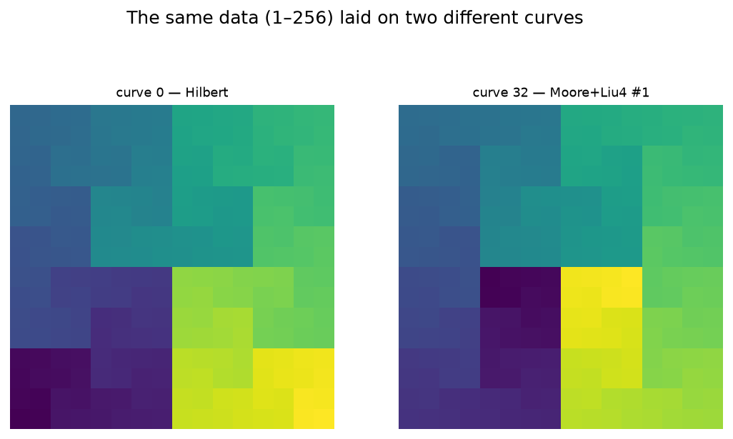
*The same numbers on curve 0 and curve 32 — one reason to have all forty.*
|
|
116
|
+
|
|
117
|
+
## Seeing more than the data
|
|
118
|
+
|
|
119
|
+
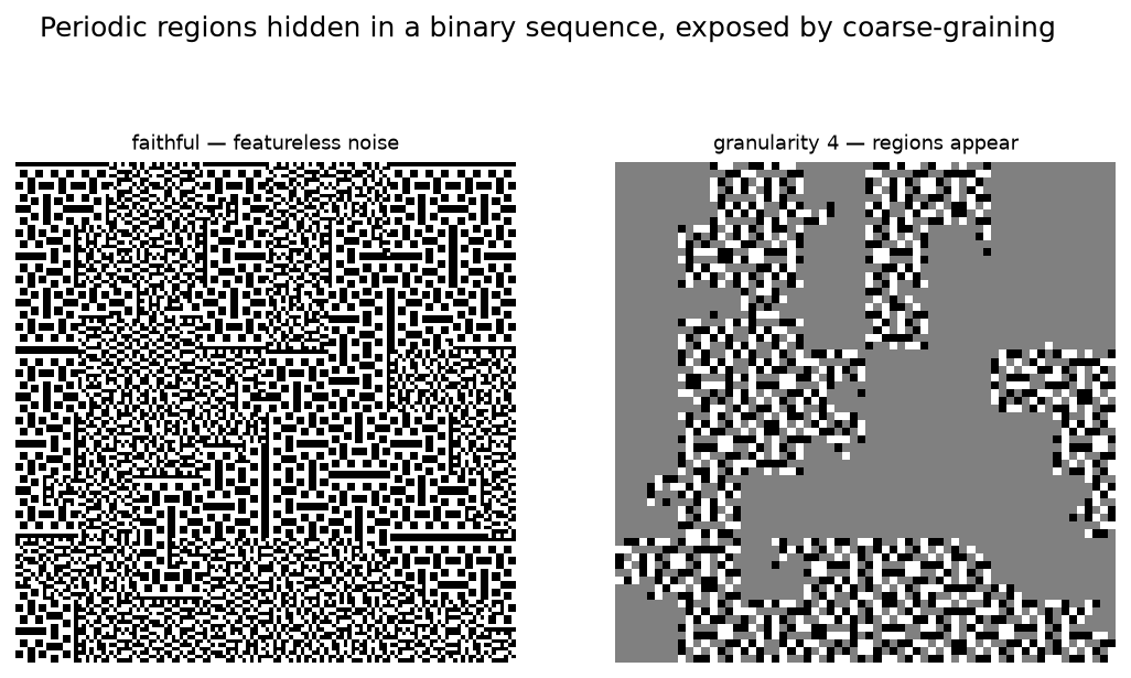
**Coarse-grain it.** `plot.show(granularity=4)` replaces each block of values by its mean.
|
|
120
|
+
Below, a binary sequence interleaves stretches of two periodic patterns with identical
|
|
121
|
+
density — invisible in the faithful plot, obvious once averaged.
|
|
122
|
+
|
|
123
|
+
|
|
124
|
+
|
|
125
|
+
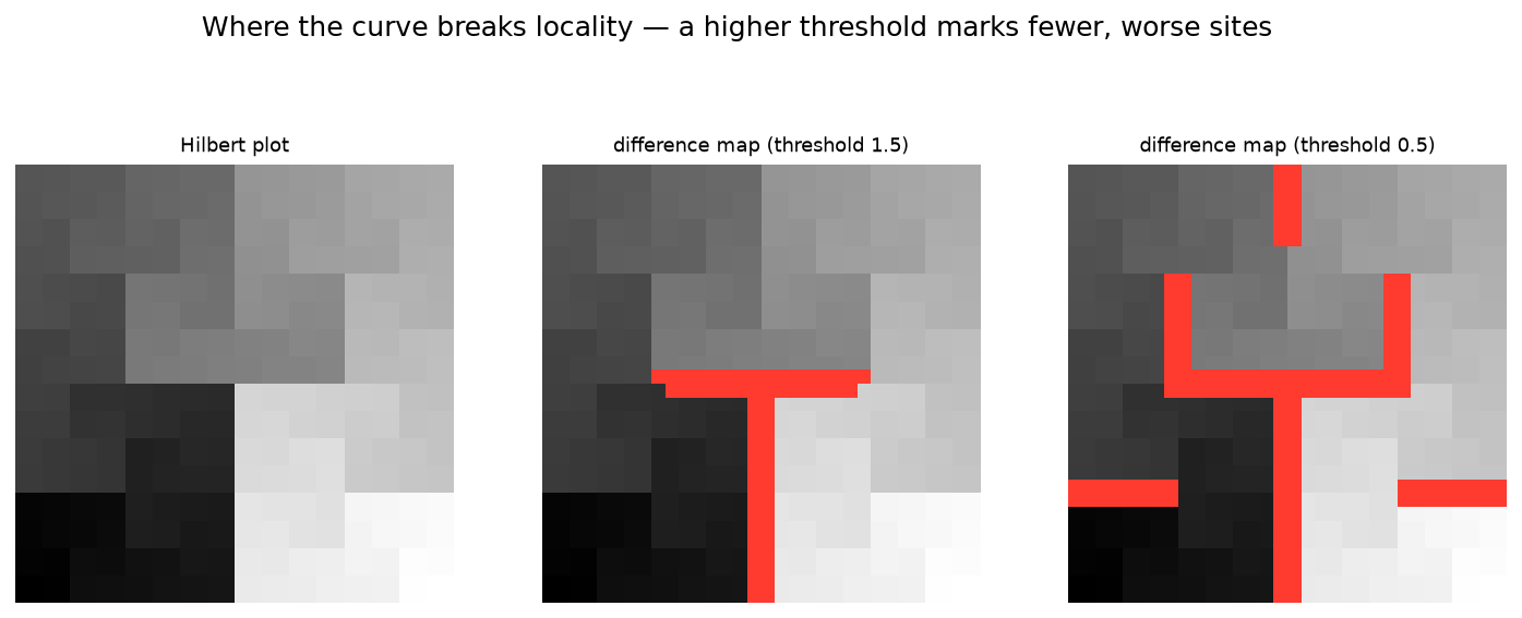
**Find where locality breaks.** `plot.show(difference=True)` marks the cells that are
|
|
126
|
+
neighbours in the plane but far apart along the curve. A higher threshold keeps only the
|
|
127
|
+
worst offenders.
|
|
128
|
+
|
|
129
|
+
|
|
130
|
+
|
|
131
|
+
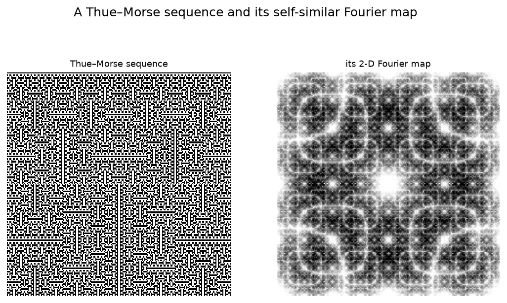
**Transform it.** `plot.show(fourier=True)` renders the 2-D Fourier map, exposing periodic
|
|
132
|
+
and self-similar structure — here, a Thue–Morse sequence.
|
|
133
|
+
|
|
134
|
+
|
|
135
|
+
|
|
136
|
+
## Also
|
|
137
|
+
|
|
138
|
+
- `curve.unroll(img)` — read a 2-D array back into 1-D, in curve order
|
|
139
|
+
- `curve.grid(n)` — the eight `generalizing()` curves tile **any** `n×n` square, not just `2ᵏ`
|
|
140
|
+
- `curve.label_map(order)` — the grid of visit indices, as an image
|
|
141
|
+
- `curve.difference_map(order)` — where the curve breaks locality, as a field
|
|
142
|
+
- `plot.draw(colorbar=True)`, or `norm=LogNorm()` for heavy-tailed data
|
|
143
|
+
- `hilbertplot.is_space_filling` / `canonical_form` — check a path yourself; the same tools
|
|
144
|
+
the test suite uses to prove all forty curves are distinct Hamiltonian paths
|
|
145
|
+
- `hilbertplot.clear_cache()` / `cache_info()` — generated curves are memoised; this frees them
|
|
146
|
+
- `hilbertplot.set_cell_limit(n)` — raise the guard that refuses absurdly large orders
|
|
147
|
+
|
|
148
|
+
Every figure above is reproducible: `python examples/readme_figures.py`. More runnable
|
|
149
|
+
demos are in
|
|
150
|
+
[`examples/`](https://github.com/El3ssar/hilbertplot/tree/main/examples);
|
|
151
|
+
the arbitrary-square classification and its impossibility proofs are in the repository's
|
|
152
|
+
`research/quasisquares/`.
|
|
153
|
+
|
|
154
|
+
## License
|
|
155
|
+
|
|
156
|
+
MIT © Daniel Estevez —
|
|
157
|
+
[LICENSE](https://github.com/El3ssar/hilbertplot/blob/main/LICENSE)
|
|
@@ -0,0 +1,124 @@
|
|
|
1
|
+
# hilbertplot
|
|
2
|
+
|
|
3
|
+
[](https://pypi.org/project/hilbertplot/)
|
|
4
|
+
[](https://github.com/El3ssar/hilbertplot/actions/workflows/ci.yml)
|
|
5
|
+
[](https://pypi.org/project/hilbertplot/)
|
|
6
|
+
[](https://github.com/El3ssar/hilbertplot/blob/main/LICENSE)
|
|
7
|
+
|
|
8
|
+
The **complete set of 40 two-dimensional Hilbert curves** — and a fast way to plot long
|
|
9
|
+
1-D data on any of them.
|
|
10
|
+
|
|
11
|
+
Most software knows one Hilbert curve. In fact there are **forty** distinct space-filling
|
|
12
|
+
curves of Hilbert type in two dimensions (up to rotation, reflection and reversion), as
|
|
13
|
+
proved by Estevez-Rams et al., *"Hilbert curves in two dimensions"*, Rev. Cub. Fís. **34**,
|
|
14
|
+
9 (2017). `hilbertplot` implements all forty with pure-numpy generation and uses them to lay
|
|
15
|
+
long 1-D vectors onto 2-D images.
|
|
16
|
+
|
|
17
|
+
<p align="center">
|
|
18
|
+
<img src="https://raw.githubusercontent.com/El3ssar/hilbertplot/main/assets/curve.png"
|
|
19
|
+
width="440" alt="The Hilbert curve at order 4, drawn as a colour-graded path">
|
|
20
|
+
</p>
|
|
21
|
+
|
|
22
|
+
## Install
|
|
23
|
+
|
|
24
|
+
```bash
|
|
25
|
+
pip install "hilbertplot[plot]" # drop [plot] for a numpy-only core (no matplotlib)
|
|
26
|
+
```
|
|
27
|
+
|
|
28
|
+
## Draw a curve
|
|
29
|
+
|
|
30
|
+
```python
|
|
31
|
+
import hilbertplot
|
|
32
|
+
|
|
33
|
+
c = hilbertplot.curve(0) # by index 0–39, by name ("Moore"), or by symbol
|
|
34
|
+
c.show(4) # draw order 4 in a window
|
|
35
|
+
pts = c.points(4) # (256, 2) integer lattice points, in visit order
|
|
36
|
+
```
|
|
37
|
+
|
|
38
|
+
The forty curves come in named groups — `hilbertplot.proper()`, `.improper()`,
|
|
39
|
+
`.homogeneous()`, `.inhomogeneous()`, `.generalizing()` — each of which prints as a table,
|
|
40
|
+
and which compose:
|
|
41
|
+
|
|
42
|
+
```python
|
|
43
|
+
import hilbertplot
|
|
44
|
+
|
|
45
|
+
print(hilbertplot.proper()) # a table of the six proper curves
|
|
46
|
+
hilbertplot.catalog().closed().names # ['Moore', 'Liu1', 'Improper1', 'Improper4']
|
|
47
|
+
hilbertplot.by_kernels(3, 5).gallery(order=3) # draw a group as a grid of panels
|
|
48
|
+
```
|
|
49
|
+
|
|
50
|
+
In a Jupyter notebook a `Curve` renders itself — put `hilbertplot.curve("Moore")` in a cell
|
|
51
|
+
and you get the picture, not a `repr`.
|
|
52
|
+
|
|
53
|
+
## One cell at a time
|
|
54
|
+
|
|
55
|
+
`points(order)` builds all `4**order` cells. When you only need *where step `i` lands*,
|
|
56
|
+
`encode` answers in `O(order)` — so it works at orders no machine could materialise, and it
|
|
57
|
+
does so for **all forty** curves, not just the classic one:
|
|
58
|
+
|
|
59
|
+
```python
|
|
60
|
+
import hilbertplot
|
|
61
|
+
|
|
62
|
+
c = hilbertplot.curve(0)
|
|
63
|
+
c.encode(5, 2) # (0, 3) — the cell visited at step 5, order 2
|
|
64
|
+
c.decode(0, 3, 2) # 5 — and back again
|
|
65
|
+
c.encode(10**18, 40) # (751054336, 346100736) — a 2**80-cell curve
|
|
66
|
+
```
|
|
67
|
+
|
|
68
|
+
## Plot data
|
|
69
|
+
|
|
70
|
+
Walk a curve and drop `data[i]` on the *i*-th cell it visits: a locality-preserving
|
|
71
|
+
1-D → 2-D map where nearby values stay nearby.
|
|
72
|
+
|
|
73
|
+
```python
|
|
74
|
+
import numpy as np, hilbertplot
|
|
75
|
+
|
|
76
|
+
plot = hilbertplot.hilbert_plot(0, np.arange(1, 257))
|
|
77
|
+
plot.show("viridis") # a matplotlib colormap name, or a list of colours to blend
|
|
78
|
+
```
|
|
79
|
+
|
|
80
|
+

|
|
81
|
+
|
|
82
|
+
*The same numbers on curve 0 and curve 32 — one reason to have all forty.*
|
|
83
|
+
|
|
84
|
+
## Seeing more than the data
|
|
85
|
+
|
|
86
|
+
**Coarse-grain it.** `plot.show(granularity=4)` replaces each block of values by its mean.
|
|
87
|
+
Below, a binary sequence interleaves stretches of two periodic patterns with identical
|
|
88
|
+
density — invisible in the faithful plot, obvious once averaged.
|
|
89
|
+
|
|
90
|
+

|
|
91
|
+
|
|
92
|
+
**Find where locality breaks.** `plot.show(difference=True)` marks the cells that are
|
|
93
|
+
neighbours in the plane but far apart along the curve. A higher threshold keeps only the
|
|
94
|
+
worst offenders.
|
|
95
|
+
|
|
96
|
+

|
|
97
|
+
|
|
98
|
+
**Transform it.** `plot.show(fourier=True)` renders the 2-D Fourier map, exposing periodic
|
|
99
|
+
and self-similar structure — here, a Thue–Morse sequence.
|
|
100
|
+
|
|
101
|
+

|
|
102
|
+
|
|
103
|
+
## Also
|
|
104
|
+
|
|
105
|
+
- `curve.unroll(img)` — read a 2-D array back into 1-D, in curve order
|
|
106
|
+
- `curve.grid(n)` — the eight `generalizing()` curves tile **any** `n×n` square, not just `2ᵏ`
|
|
107
|
+
- `curve.label_map(order)` — the grid of visit indices, as an image
|
|
108
|
+
- `curve.difference_map(order)` — where the curve breaks locality, as a field
|
|
109
|
+
- `plot.draw(colorbar=True)`, or `norm=LogNorm()` for heavy-tailed data
|
|
110
|
+
- `hilbertplot.is_space_filling` / `canonical_form` — check a path yourself; the same tools
|
|
111
|
+
the test suite uses to prove all forty curves are distinct Hamiltonian paths
|
|
112
|
+
- `hilbertplot.clear_cache()` / `cache_info()` — generated curves are memoised; this frees them
|
|
113
|
+
- `hilbertplot.set_cell_limit(n)` — raise the guard that refuses absurdly large orders
|
|
114
|
+
|
|
115
|
+
Every figure above is reproducible: `python examples/readme_figures.py`. More runnable
|
|
116
|
+
demos are in
|
|
117
|
+
[`examples/`](https://github.com/El3ssar/hilbertplot/tree/main/examples);
|
|
118
|
+
the arbitrary-square classification and its impossibility proofs are in the repository's
|
|
119
|
+
`research/quasisquares/`.
|
|
120
|
+
|
|
121
|
+
## License
|
|
122
|
+
|
|
123
|
+
MIT © Daniel Estevez —
|
|
124
|
+
[LICENSE](https://github.com/El3ssar/hilbertplot/blob/main/LICENSE)
|
|
@@ -35,7 +35,7 @@ def main() -> None:
|
|
|
35
35
|
title="All 40 two-dimensional Hilbert curves (order 3)",
|
|
36
36
|
save=os.path.join(OUT, "all40.png"),
|
|
37
37
|
)
|
|
38
|
-
hp.curve(0).save(
|
|
38
|
+
hp.curve(0).save(os.path.join(OUT, "hilbert_order6.png"), 6)
|
|
39
39
|
print(f"wrote plots to {OUT}")
|
|
40
40
|
|
|
41
41
|
|
|
@@ -0,0 +1,128 @@
|
|
|
1
|
+
"""Regenerate the figures shown in the README.
|
|
2
|
+
|
|
3
|
+
python examples/readme_figures.py
|
|
4
|
+
|
|
5
|
+
Writes to assets/:
|
|
6
|
+
* curve.png -- curve 0 at order 4, drawn as a colour-graded path
|
|
7
|
+
* data_two_curves.png -- the numbers 1-256 laid on curve 0 and on curve 32
|
|
8
|
+
* difference.png -- the difference-map overlay at two thresholds
|
|
9
|
+
* thue_morse.png -- a Thue-Morse sequence and its 2-D Fourier map
|
|
10
|
+
* granularity.png -- periodic regions that only appear once coarse-grained
|
|
11
|
+
"""
|
|
12
|
+
|
|
13
|
+
import os
|
|
14
|
+
|
|
15
|
+
import numpy as np
|
|
16
|
+
|
|
17
|
+
import hilbertplot as hp
|
|
18
|
+
|
|
19
|
+
OUT = os.path.join(os.path.dirname(__file__), "..", "assets")
|
|
20
|
+
|
|
21
|
+
|
|
22
|
+
def thue_morse(n):
|
|
23
|
+
"""The first ``n`` terms of the Thue-Morse sequence."""
|
|
24
|
+
s = [0]
|
|
25
|
+
while len(s) < n:
|
|
26
|
+
s = s + [1 - x for x in s]
|
|
27
|
+
return np.array(s[:n], dtype=float)
|
|
28
|
+
|
|
29
|
+
|
|
30
|
+
def interleaved_periodic(n, seed=3):
|
|
31
|
+
"""A random interleaving of two periodic patterns of *equal* density.
|
|
32
|
+
|
|
33
|
+
``.1001.`` (period 4) and ``.110100.`` (period 6) both have density 1/2, so no
|
|
34
|
+
stretch is brighter than another and the faithful plot is featureless noise. Every
|
|
35
|
+
chunk length is a multiple of 12, which keeps chunk starts aligned to the
|
|
36
|
+
granularity-4 block grid -- so 4-granularity collapses the period-4 stretches to a
|
|
37
|
+
constant (solid blocks) while the period-6 ones keep varying.
|
|
38
|
+
"""
|
|
39
|
+
p4, p6 = [1, 0, 0, 1], [1, 1, 0, 1, 0, 0]
|
|
40
|
+
rng = np.random.default_rng(seed)
|
|
41
|
+
seq = []
|
|
42
|
+
while len(seq) < n:
|
|
43
|
+
p = p4 if rng.integers(2) else p6
|
|
44
|
+
length = 12 * int(rng.integers(16, 110))
|
|
45
|
+
seq += (p * (-(-length // len(p))))[:length]
|
|
46
|
+
return np.array(seq[:n], dtype=float)
|
|
47
|
+
|
|
48
|
+
|
|
49
|
+
def main() -> None:
|
|
50
|
+
import matplotlib
|
|
51
|
+
|
|
52
|
+
matplotlib.use("Agg")
|
|
53
|
+
import matplotlib.pyplot as plt
|
|
54
|
+
|
|
55
|
+
os.makedirs(OUT, exist_ok=True)
|
|
56
|
+
plt.rcParams.update({"figure.facecolor": "white", "savefig.facecolor": "white"})
|
|
57
|
+
|
|
58
|
+
def save(fig, name, dpi=140):
|
|
59
|
+
fig.savefig(os.path.join(OUT, name), dpi=dpi, bbox_inches="tight")
|
|
60
|
+
plt.close(fig)
|
|
61
|
+
|
|
62
|
+
# 1) the curve itself, colour-graded along the traversal
|
|
63
|
+
fig, ax = plt.subplots(figsize=(5.2, 5.2))
|
|
64
|
+
hp.curve(0).draw(4, ax=ax, cmap="viridis", title="The Hilbert curve (curve 0), order 4")
|
|
65
|
+
save(fig, "curve.png")
|
|
66
|
+
|
|
67
|
+
# 2) the same data laid on two different curves
|
|
68
|
+
data = np.arange(1, 257)
|
|
69
|
+
fig, axes = plt.subplots(1, 2, figsize=(9.2, 4.9))
|
|
70
|
+
hp.hilbert_plot(0, data).draw("viridis", ax=axes[0], title="curve 0 — Hilbert")
|
|
71
|
+
hp.hilbert_plot(32, data).draw("viridis", ax=axes[1], title="curve 32 — Moore+Liu4 #1")
|
|
72
|
+
fig.suptitle("The same data (1–256) laid on two different curves", fontsize=13, y=1.02)
|
|
73
|
+
save(fig, "data_two_curves.png")
|
|
74
|
+
|
|
75
|
+
# 3) where the curve breaks locality, at two thresholds
|
|
76
|
+
plot = hp.hilbert_plot(0, np.arange(4**5))
|
|
77
|
+
fig, axes = plt.subplots(1, 3, figsize=(12.6, 4.6))
|
|
78
|
+
plot.draw("gray", ax=axes[0], title="Hilbert plot")
|
|
79
|
+
for ax, thr in ((axes[1], 1.5), (axes[2], 0.5)):
|
|
80
|
+
plot.draw(
|
|
81
|
+
"gray",
|
|
82
|
+
ax=ax,
|
|
83
|
+
difference=True,
|
|
84
|
+
difference_threshold=thr,
|
|
85
|
+
difference_color="#ff3b30",
|
|
86
|
+
title=f"difference map (threshold {thr})",
|
|
87
|
+
)
|
|
88
|
+
fig.suptitle(
|
|
89
|
+
"Where the curve breaks locality — a higher threshold marks fewer, worse sites",
|
|
90
|
+
fontsize=13,
|
|
91
|
+
y=1.02,
|
|
92
|
+
)
|
|
93
|
+
save(fig, "difference.png")
|
|
94
|
+
|
|
95
|
+
# 4) a Thue-Morse sequence and its Fourier map (paper-style: light ground)
|
|
96
|
+
plot = hp.hilbert_plot(0, thue_morse(4**8))
|
|
97
|
+
fig, axes = plt.subplots(1, 2, figsize=(9.2, 4.9))
|
|
98
|
+
plot.draw("gray", ax=axes[0], title="Thue–Morse sequence")
|
|
99
|
+
lo, hi = np.percentile(plot.fourier(window=True), [2.0, 99.5])
|
|
100
|
+
plot.draw(
|
|
101
|
+
"gray_r",
|
|
102
|
+
ax=axes[1],
|
|
103
|
+
fourier=True,
|
|
104
|
+
window=True,
|
|
105
|
+
vmin=lo,
|
|
106
|
+
vmax=hi,
|
|
107
|
+
title="its 2-D Fourier map",
|
|
108
|
+
)
|
|
109
|
+
fig.suptitle("A Thue–Morse sequence and its self-similar Fourier map", fontsize=13, y=1.02)
|
|
110
|
+
save(fig, "thue_morse.png")
|
|
111
|
+
|
|
112
|
+
# 5) periodic regions that only show up once you coarse-grain
|
|
113
|
+
plot = hp.hilbert_plot(0, interleaved_periodic(4**7))
|
|
114
|
+
fig, axes = plt.subplots(1, 2, figsize=(9.2, 4.9))
|
|
115
|
+
plot.draw("gray", ax=axes[0], title="faithful — featureless noise")
|
|
116
|
+
plot.draw("gray", ax=axes[1], granularity=4, title="granularity 4 — regions appear")
|
|
117
|
+
fig.suptitle(
|
|
118
|
+
"Periodic regions hidden in a binary sequence, exposed by coarse-graining",
|
|
119
|
+
fontsize=13,
|
|
120
|
+
y=1.02,
|
|
121
|
+
)
|
|
122
|
+
save(fig, "granularity.png")
|
|
123
|
+
|
|
124
|
+
print(f"wrote README figures to {os.path.normpath(OUT)}")
|
|
125
|
+
|
|
126
|
+
|
|
127
|
+
if __name__ == "__main__":
|
|
128
|
+
main()
|
|
@@ -4,11 +4,14 @@ build-backend = "hatchling.build"
|
|
|
4
4
|
|
|
5
5
|
[project]
|
|
6
6
|
name = "hilbertplot"
|
|
7
|
-
version = "0.
|
|
7
|
+
version = "0.2.0"
|
|
8
8
|
description = "The complete set of 40 two-dimensional Hilbert curves, and data plots on them."
|
|
9
9
|
readme = "README.md"
|
|
10
10
|
requires-python = ">=3.10"
|
|
11
|
-
license
|
|
11
|
+
# PEP 639: a license expression plus the file, instead of the deprecated
|
|
12
|
+
# `license = { text = ... }` + `License ::` classifier pair.
|
|
13
|
+
license = "MIT"
|
|
14
|
+
license-files = ["LICENSE"]
|
|
12
15
|
authors = [{ name = "Daniel Estevez", email = "kemossabee@gmail.com" }]
|
|
13
16
|
keywords = [
|
|
14
17
|
"hilbert-curve",
|
|
@@ -19,10 +22,14 @@ keywords = [
|
|
|
19
22
|
"visualization",
|
|
20
23
|
]
|
|
21
24
|
classifiers = [
|
|
22
|
-
"Development Status ::
|
|
25
|
+
"Development Status :: 4 - Beta",
|
|
23
26
|
"Intended Audience :: Science/Research",
|
|
24
|
-
"License :: OSI Approved :: MIT License",
|
|
25
27
|
"Programming Language :: Python :: 3",
|
|
28
|
+
"Programming Language :: Python :: 3.10",
|
|
29
|
+
"Programming Language :: Python :: 3.11",
|
|
30
|
+
"Programming Language :: Python :: 3.12",
|
|
31
|
+
"Programming Language :: Python :: 3.13",
|
|
32
|
+
"Programming Language :: Python :: 3.14",
|
|
26
33
|
"Topic :: Scientific/Engineering :: Mathematics",
|
|
27
34
|
"Topic :: Scientific/Engineering :: Visualization",
|
|
28
35
|
"Typing :: Typed",
|
|
@@ -31,12 +38,14 @@ dependencies = ["numpy>=1.21"]
|
|
|
31
38
|
|
|
32
39
|
[project.optional-dependencies]
|
|
33
40
|
plot = ["matplotlib>=3.5"]
|
|
34
|
-
dev
|
|
41
|
+
# dev composes [plot] rather than restating matplotlib, so the two cannot drift.
|
|
42
|
+
dev = ["hilbertplot[plot]", "pytest>=7.0", "ruff==0.15.13"]
|
|
35
43
|
|
|
36
44
|
[project.urls]
|
|
37
45
|
Homepage = "https://github.com/El3ssar/hilbertplot"
|
|
38
46
|
Source = "https://github.com/El3ssar/hilbertplot"
|
|
39
47
|
Issues = "https://github.com/El3ssar/hilbertplot/issues"
|
|
48
|
+
Changelog = "https://github.com/El3ssar/hilbertplot/blob/main/CHANGELOG.md"
|
|
40
49
|
|
|
41
50
|
[tool.hatch.build.targets.wheel]
|
|
42
51
|
packages = ["src/hilbertplot"]
|
|
@@ -49,11 +58,16 @@ include = [
|
|
|
49
58
|
"/tests",
|
|
50
59
|
"/examples/*.py",
|
|
51
60
|
"/README.md",
|
|
61
|
+
"/CHANGELOG.md",
|
|
52
62
|
"/LICENSE",
|
|
53
63
|
]
|
|
54
64
|
|
|
55
65
|
[tool.pytest.ini_options]
|
|
56
66
|
testpaths = ["tests"]
|
|
67
|
+
# `-W error::RuntimeWarning` turns any numpy RuntimeWarning raised during the suite into a
|
|
68
|
+
# failure: an "invalid value encountered in divide" during ordinary use is a defect, not
|
|
69
|
+
# noise. (The README's own snippets are executed by tests/test_readme.py.)
|
|
70
|
+
addopts = "-W error::RuntimeWarning"
|
|
57
71
|
|
|
58
72
|
[tool.ruff]
|
|
59
73
|
line-length = 100
|
|
@@ -62,19 +76,15 @@ line-length = 100
|
|
|
62
76
|
extend-exclude = ["research/"]
|
|
63
77
|
|
|
64
78
|
[tool.ruff.lint]
|
|
65
|
-
|
|
79
|
+
# RUF/SIM/C4/RET/PERF/NPY/PT are all near-zero-noise on this codebase and catch the
|
|
80
|
+
# classes of drift that actually bit us: unsorted __all__, stale noqa, over-broad
|
|
81
|
+
# pytest.raises, and numpy-specific footguns. ANN/D are deliberately NOT enabled --
|
|
82
|
+
# they would flag 390 sites without improving anything.
|
|
83
|
+
select = ["E", "F", "I", "UP", "B", "W", "RUF", "SIM", "C4", "RET", "PERF", "NPY", "PT"]
|
|
66
84
|
|
|
67
85
|
[tool.ruff.lint.per-file-ignores]
|
|
68
|
-
#
|
|
69
|
-
"
|
|
70
|
-
# the paper's parameter name `l` (ambiguous-variable-name)
|
|
71
|
-
"src/hilbertplot/_data/mapping.py" = ["E741"]
|
|
72
|
-
|
|
73
|
-
[tool.ruff.format]
|
|
74
|
-
# arbitrary.py's `_fill` is a deliberately dense, hand-tuned hot loop; keep it
|
|
75
|
-
# linted (with E701/E702 ignored above) but exempt from the formatter so its
|
|
76
|
-
# compact one-liners survive.
|
|
77
|
-
exclude = ["src/hilbertplot/_core/arbitrary.py"]
|
|
86
|
+
# examples use en dashes in figure titles on purpose (RUF001 ambiguous-unicode)
|
|
87
|
+
"examples/*.py" = ["RUF001"]
|
|
78
88
|
|
|
79
89
|
[tool.semantic_release]
|
|
80
90
|
# pyproject keeps a STATIC version = "0.1.0"; PSR stamps BOTH files in sync on
|