gaca 1.2.0__tar.gz
This diff represents the content of publicly available package versions that have been released to one of the supported registries. The information contained in this diff is provided for informational purposes only and reflects changes between package versions as they appear in their respective public registries.
- gaca-1.2.0/LICENSE +21 -0
- gaca-1.2.0/PKG-INFO +541 -0
- gaca-1.2.0/README.md +502 -0
- gaca-1.2.0/gaca/__init__.py +18 -0
- gaca-1.2.0/gaca/auto.py +881 -0
- gaca-1.2.0/gaca/cli.py +150 -0
- gaca-1.2.0/gaca/genesis.py +348 -0
- gaca-1.2.0/gaca/model.py +393 -0
- gaca-1.2.0/gaca/report.py +287 -0
- gaca-1.2.0/gaca.egg-info/PKG-INFO +541 -0
- gaca-1.2.0/gaca.egg-info/SOURCES.txt +18 -0
- gaca-1.2.0/gaca.egg-info/dependency_links.txt +1 -0
- gaca-1.2.0/gaca.egg-info/entry_points.txt +2 -0
- gaca-1.2.0/gaca.egg-info/requires.txt +18 -0
- gaca-1.2.0/gaca.egg-info/top_level.txt +1 -0
- gaca-1.2.0/pyproject.toml +61 -0
- gaca-1.2.0/setup.cfg +4 -0
- gaca-1.2.0/tests/test_auto.py +170 -0
- gaca-1.2.0/tests/test_model.py +81 -0
- gaca-1.2.0/tests/test_physics.py +96 -0
gaca-1.2.0/LICENSE
ADDED
|
@@ -0,0 +1,21 @@
|
|
|
1
|
+
MIT License
|
|
2
|
+
|
|
3
|
+
Copyright (c) 2025 henrivuorinen
|
|
4
|
+
|
|
5
|
+
Permission is hereby granted, free of charge, to any person obtaining a copy
|
|
6
|
+
of this software and associated documentation files (the "Software"), to deal
|
|
7
|
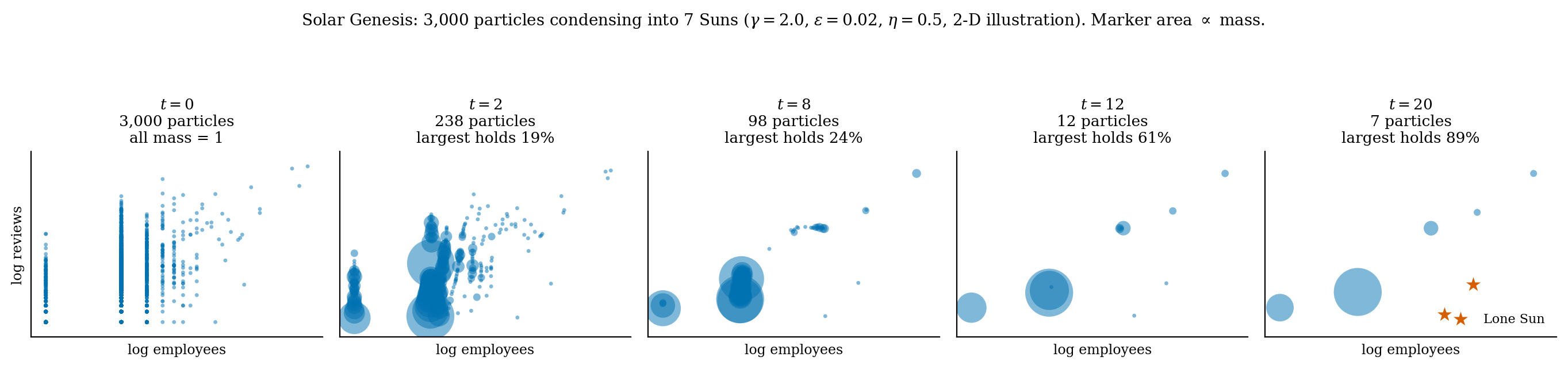
+
in the Software without restriction, including without limitation the rights
|
|
8
|
+
to use, copy, modify, merge, publish, distribute, sublicense, and/or sell
|
|
9
|
+
copies of the Software, and to permit persons to whom the Software is
|
|
10
|
+
furnished to do so, subject to the following conditions:
|
|
11
|
+
|
|
12
|
+
The above copyright notice and this permission notice shall be included in all
|
|
13
|
+
copies or substantial portions of the Software.
|
|
14
|
+
|
|
15
|
+
THE SOFTWARE IS PROVIDED "AS IS", WITHOUT WARRANTY OF ANY KIND, EXPRESS OR
|
|
16
|
+
IMPLIED, INCLUDING BUT NOT LIMITED TO THE WARRANTIES OF MERCHANTABILITY,
|
|
17
|
+
FITNESS FOR A PARTICULAR PURPOSE AND NONINFRINGEMENT. IN NO EVENT SHALL THE
|
|
18
|
+
AUTHORS OR COPYRIGHT HOLDERS BE LIABLE FOR ANY CLAIM, DAMAGES OR OTHER
|
|
19
|
+
LIABILITY, WHETHER IN AN ACTION OF CONTRACT, TORT OR OTHERWISE, ARISING FROM,
|
|
20
|
+
OUT OF OR IN CONNECTION WITH THE SOFTWARE OR THE USE OR OTHER DEALINGS IN THE
|
|
21
|
+
SOFTWARE.
|
gaca-1.2.0/PKG-INFO
ADDED
|
@@ -0,0 +1,541 @@
|
|
|
1
|
+
Metadata-Version: 2.4
|
|
2
|
+
Name: gaca
|
|
3
|
+
Version: 1.2.0
|
|
4
|
+
Summary: Gravitational Accretion Clustering: physics-inspired clustering and anomaly detection for large tables
|
|
5
|
+
Author: Henri J. Vuorinen
|
|
6
|
+
License-Expression: MIT
|
|
7
|
+
Project-URL: Homepage, https://github.com/henrivuorinen/GACA
|
|
8
|
+
Project-URL: Repository, https://github.com/henrivuorinen/GACA
|
|
9
|
+
Project-URL: Issues, https://github.com/henrivuorinen/GACA/issues
|
|
10
|
+
Project-URL: Changelog, https://github.com/henrivuorinen/GACA/blob/main/CHANGELOG.md
|
|
11
|
+
Keywords: clustering,anomaly detection,outlier detection,mean shift,density clustering,unsupervised learning,streaming
|
|
12
|
+
Classifier: Development Status :: 4 - Beta
|
|
13
|
+
Classifier: Intended Audience :: Science/Research
|
|
14
|
+
Classifier: Intended Audience :: Developers
|
|
15
|
+
Classifier: Operating System :: OS Independent
|
|
16
|
+
Classifier: Programming Language :: Python :: 3
|
|
17
|
+
Classifier: Topic :: Scientific/Engineering :: Information Analysis
|
|
18
|
+
Classifier: Topic :: Scientific/Engineering :: Artificial Intelligence
|
|
19
|
+
Classifier: Topic :: Scientific/Engineering :: Astronomy
|
|
20
|
+
Requires-Python: >=3.10
|
|
21
|
+
Description-Content-Type: text/markdown
|
|
22
|
+
License-File: LICENSE
|
|
23
|
+
Requires-Dist: numpy>=1.24
|
|
24
|
+
Requires-Dist: scipy>=1.10
|
|
25
|
+
Requires-Dist: scikit-learn>=1.3
|
|
26
|
+
Requires-Dist: pandas>=2.0
|
|
27
|
+
Provides-Extra: cli
|
|
28
|
+
Provides-Extra: experiments
|
|
29
|
+
Requires-Dist: matplotlib>=3.7; extra == "experiments"
|
|
30
|
+
Requires-Dist: hdbscan>=0.8; extra == "experiments"
|
|
31
|
+
Requires-Dist: lightgbm>=4.0; extra == "experiments"
|
|
32
|
+
Requires-Dist: psutil>=5.9; extra == "experiments"
|
|
33
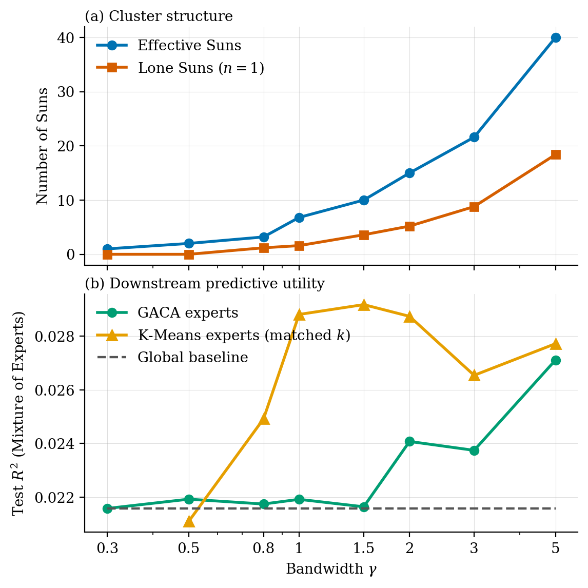
|
+
Requires-Dist: pyarrow>=14; extra == "experiments"
|
|
34
|
+
Provides-Extra: dev
|
|
35
|
+
Requires-Dist: pytest>=7; extra == "dev"
|
|
36
|
+
Requires-Dist: build; extra == "dev"
|
|
37
|
+
Requires-Dist: twine; extra == "dev"
|
|
38
|
+
Dynamic: license-file
|
|
39
|
+
|
|
40
|
+
# GACA: Gravitational Accretion Clustering Algorithm
|
|
41
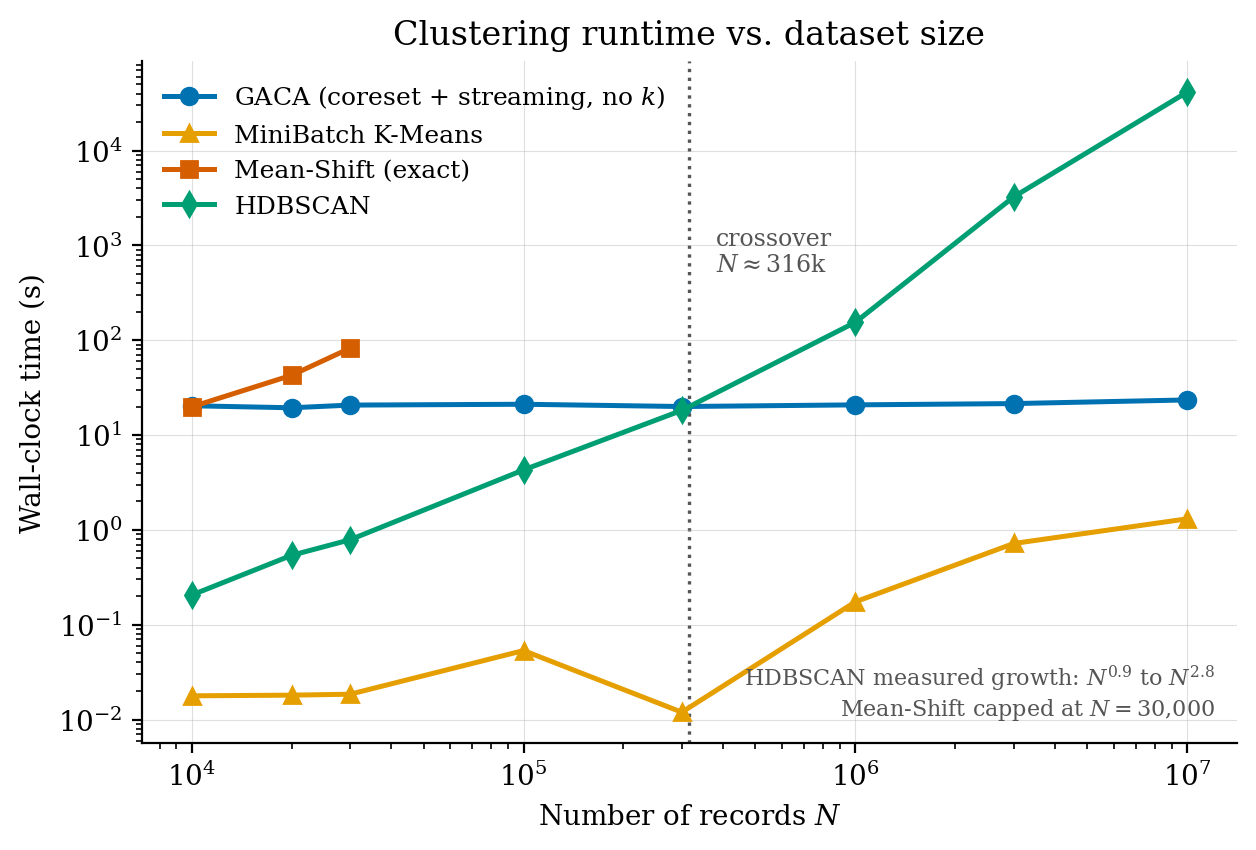
|
+
|
|
42
|
+
GACA is a density-based clustering method that treats every data point as a
|
|
43
|
+
particle with mass. Nearby mass attracts, particles drift towards dense regions,
|
|
44
|
+
and particles that meet merge and keep their combined mass. What is left are the
|
|
45
|
+
**Suns**: the cluster centres. You never specify the number of clusters. It
|
|
46
|
+
emerges from the dynamics and is controlled by one bandwidth parameter, γ.
|
|
47
|
+
|
|
48
|
+
GACA is designed for large tables. The expensive simulation runs once on a small
|
|
49
|
+
random sample (the coreset), and the full dataset is then streamed through the
|
|
50
|
+
resulting Suns in batches. In the thesis experiments this clustered **10 million
|
|
51
|
+
records in about 23 seconds on a laptop, with constant memory**.
|
|
52
|
+
|
|
53
|
+
This repository contains the reference implementation from the master's thesis
|
|
54
|
+
*The Gravitational Accretion Clustering Algorithm (GACA): Scalable,
|
|
55
|
+
Physics-Inspired Clustering for Large Datasets*, plus several improvements made
|
|
56
|
+
after it (see [Improvements since the thesis](#improvements-since-the-thesis)).
|
|
57
|
+
The thesis behaviour is still available with
|
|
58
|
+
`GACA(assignment='newton', method='barnes_hut')`, and every script in
|
|
59
|
+
`experiments/` uses it.
|
|
60
|
+
|
|
61
|
+
|
|
62
|
+
|
|
63
|
+
## How it works
|
|
64
|
+
|
|
65
|
+
**Phase 1: Solar Genesis (structure discovery on a coreset).** A uniform sample of
|
|
66
|
+
`sample_size` rows (5,000 by default) starts as particles of mass 1. Each
|
|
67
|
+
iteration:
|
|
68
|
+
|
|
69
|
+
1. **Transport.** Every particle moves a damped step (η) towards the mass-weighted
|
|
70
|
+
Gaussian average of its surroundings. This is exactly a blurring mean-shift
|
|
71
|
+
step: the displacement equals `(1 / 2γ) ∇ log KDE(x)`.
|
|
72
|
+
2. **Condensation.** Particles closer than ε are linked, and each connected
|
|
73
|
+
component is replaced by one particle at its centre of mass, carrying the
|
|
74
|
+
summed mass. Mass is conserved exactly.
|
|
75
|
+
|
|
76
|
+
The Gaussian sum is evaluated exactly in vectorised blocks (`method='exact'`,
|
|
77
|
+
the default). The thesis used a Barnes-Hut tree (`method='barnes_hut'`), which is
|
|
78
|
+
asymptotically cheaper but in interpreted Python is 90 to 140 times slower on
|
|
79
|
+
the coresets GACA uses, and only approximate. Genesis stops at a stable plateau
|
|
80
|
+
or at the iteration cap. The surviving particles are the Suns, and every
|
|
81
|
+
coreset row remembers which Sun it condensed into.
|
|
82
|
+
|
|
83
|
+
**Phase 2: Particle Accretion (assignment of every row).** Each row is assigned
|
|
84
|
+
to the Sun whose coreset members exert the strongest Gaussian pull on it,
|
|
85
|
+
`Σ_{j ∈ Sun k} exp(−γ‖x − z_j‖²)`, summed over its 32 nearest coreset members.
|
|
86
|
+
This follows the shape the dynamics found rather than cutting space into
|
|
87
|
+
Voronoi cells. It is O(N log n_c) time and works batch by batch, so memory
|
|
88
|
+
depends on the batch size rather than on N. (`assignment='newton'` restores
|
|
89
|
+
the thesis rule, `M_k / d²`.)
|
|
90
|
+
|
|
91
|
+
**Lone Suns (anomalies).** A point far from everything feels essentially no
|
|
92
|
+
Gaussian pull, never moves and never merges. It survives as a Sun of mass 1: a
|
|
93
|
+
Lone Sun. Assignment applies the same test to every streamed row: if the total
|
|
94
|
+
pull on it is below `kappa_`, the row would not have moved had it been in the
|
|
95
|
+
coreset (thesis Prop. 3.8), so it becomes a new Lone Sun, or joins an earlier
|
|
96
|
+
Lone Sun that pulls it. Anomalies therefore no longer need to be in the coreset
|
|
97
|
+
to be isolated.
|
|
98
|
+
|
|
99
|
+
**Saddle linking (optional, `link_tau`).** At a fine bandwidth a curved or
|
|
100
|
+
elongated cluster splits into a chain of Suns. With `link_tau` set, two Suns
|
|
101
|
+
are joined when the density along the best edge between their members stays
|
|
102
|
+
above `link_tau` times the lower of their two peaks, so the decision rests on
|
|
103
|
+
the mass lying between the Suns rather than the distance between them. Lone
|
|
104
|
+
Suns are never joined.
|
|
105
|
+
|
|
106
|
+
## Installation
|
|
107
|
+
|
|
108
|
+
```bash
|
|
109
|
+
pip install gaca
|
|
110
|
+
```
|
|
111
|
+
|
|
112
|
+
That installs the package and the `gaca` command (numpy, scipy, scikit-learn
|
|
113
|
+
and pandas are pulled in). Python 3.10 or newer.
|
|
114
|
+
|
|
115
|
+
For the latest development version, or to run the tests and experiments:
|
|
116
|
+
|
|
117
|
+
```bash
|
|
118
|
+
pip install "git+https://github.com/henrivuorinen/GACA.git" # latest from GitHub
|
|
119
|
+
|
|
120
|
+
git clone https://github.com/henrivuorinen/GACA.git # or work on the code
|
|
121
|
+
cd GACA
|
|
122
|
+
pip install -e ".[dev]" # + pytest, build, twine
|
|
123
|
+
pip install -e ".[experiments]" # + matplotlib, hdbscan, lightgbm, ... for experiments/
|
|
124
|
+
```
|
|
125
|
+
|
|
126
|
+
## Any table: AutoGACA and the `gaca` command
|
|
127
|
+
|
|
128
|
+
The algorithm only needs points in a space, but someone has to decide how to
|
|
129
|
+
turn a table into that space and which bandwidth to use. `AutoGACA` makes those
|
|
130
|
+
decisions from the data and records each one, so a dataset can be clustered
|
|
131
|
+
without knowing anything about it in advance:
|
|
132
|
+
|
|
133
|
+
```bash
|
|
134
|
+
gaca run galaxies.csv # writes galaxies_gaca/
|
|
135
|
+
gaca run galaxies.csv --exclude objid,ra,dec # leave columns out
|
|
136
|
+
gaca run huge.csv --chunksize 200000 # files larger than memory
|
|
137
|
+
```
|
|
138
|
+
|
|
139
|
+
The output folder holds `labels.csv` (the input rows plus `gaca_cluster`,
|
|
140
|
+
`gaca_anomaly`, `gaca_anomaly_group` and `gaca_anomaly_score`), a self-contained
|
|
141
|
+
`report.html` and `summary.json`. The report describes each cluster in terms of
|
|
142
|
+
the original columns, lists the anomalies and the columns that make them
|
|
143
|
+
unusual, shows how the resolution was chosen and which other resolutions were
|
|
144
|
+
also stable, and lists every preprocessing decision.
|
|
145
|
+
|
|
146
|
+
From Python:
|
|
147
|
+
|
|
148
|
+
```python
|
|
149
|
+
from gaca import AutoGACA
|
|
150
|
+
|
|
151
|
+
auto = AutoGACA().fit(df) # DataFrame, array, or path to a CSV
|
|
152
|
+
print(auto.summary())
|
|
153
|
+
auto.result_ # per-row cluster, anomaly flag, group, score
|
|
154
|
+
auto.report("report.html", data=df)
|
|
155
|
+
new = auto.assign(df_new) # same preprocessing, same clusters
|
|
156
|
+
```
|
|
157
|
+
|
|
158
|
+
What it decides, and how:
|
|
159
|
+
|
|
160
|
+
| Step | Rule |
|
|
161
|
+
|---|---|
|
|
162
|
+
| Columns | Numeric columns are used. Text, identifiers (unique integers named like `id` or strictly increasing), constant columns and columns more than 50% missing are left out. `columns=` / `exclude=` override. |
|
|
163
|
+
| Missing values | Median of the column. |
|
|
164
|
+
| Transforms | `log1p` for count- or flux-like columns: non-negative, skewed, and spanning more than an order of magnitude. Other skewed columns are left alone, since a log would also pull genuine outliers back towards the data. |
|
|
165
|
+
| Scaling | Median and interquartile range, so outliers do not compress everything else. `scale='none'` (`--scale none`) keeps the values as they are, for data whose distances already mean something, such as positions in physical units. |
|
|
166
|
+
| Dimensions | Unchanged up to `max_dims` columns (default 10). Above that, PCA to between 5 and `max_dims` components, the number set by the noise floor of the singular values (Gavish and Donoho). |
|
|
167
|
+
| γ | Swept as c / (median squared distance between rows). At each value GACA is fitted on four subsamples. γ is the middle of the most stable stretch of the longest plateau in the cluster count. A split only counts if the subsamples agree (adjusted Rand index ≥ 0.8). Otherwise the answer is one group. |
|
|
168
|
+
| Anomalies | Rows that no cluster pulls, plus clusters smaller than `min_cluster_size` (10 rows). Score = −log10 of the pull relative to a typical row; above 3 is anomalous. |
|
|
169
|
+
| Hierarchy | Every stable resolution of the sweep is kept, fitted on the same coreset and nested into a tree: each fine cluster sits under the coarse cluster holding most of its particles, and each row is assigned within its own branch. `gaca_cluster` is the level the rule above picks; `gaca_level_1 … gaca_level_K` hold all levels as path-style names (`0`, `0.2`, `0.2.1`). `hierarchy=False` turns it off. |
|
|
170
|
+
|
|
171
|
+
How it did on data it was not tuned on (ARI against known labels; *best γ* is
|
|
172
|
+
the best that any γ in the sweep achieved):
|
|
173
|
+
|
|
174
|
+
| Data | Rows × columns | AutoGACA | Best γ | Notes |
|
|
175
|
+
|---|---|---|---|---|
|
|
176
|
+
| Wine | 178 × 13 | 0.79 | 0.82 | 3 clusters, PCA to 5-D |
|
|
177
|
+
| Iris | 150 × 4 | 0.54 | 0.55 | two of the species overlap; density methods see 2 groups |
|
|
178
|
+
| Breast cancer | 569 × 30 | 0.36 | 0.50 | |
|
|
179
|
+
| Blobs + planted anomalies | 20,042 × 5 | 0.99 | 0.99 | 42/42 anomalies, 0.1% false positives |
|
|
180
|
+
| 6 clusters in 30-D, 25 columns of noise | 6,000 × 30 | 0.90 | 0.89 | PCA to 5-D |
|
|
181
|
+
| Two moons, `link_tau=0.6` | 4,000 × 2 | 1.00 | | |
|
|
182
|
+
| Concentric circles, `link_tau=0.6` | 4,000 × 2 | 0.93 | | |
|
|
183
|
+
| Handwritten digits | 1,797 × 64 | 0.17 | 0.24 | not density-separated in a few dimensions |
|
|
184
|
+
| One Gaussian (no clusters) | 5,000 × 2 to 10 | 1 cluster | | correctly reports no structure and no anomalies |
|
|
185
|
+
|
|
186
|
+
`link_tau` is not on by default: it joins curved clusters but also merges
|
|
187
|
+
clusters that overlap (the 30-D case drops to 0.15 with it).
|
|
188
|
+
|
|
189
|
+
### The cluster hierarchy
|
|
190
|
+
|
|
191
|
+
Real data often has structure at several scales, and one automatic resolution
|
|
192
|
+
then has to pick between a coarse and a fine view that are almost equally
|
|
193
|
+
stable. AutoGACA keeps all of them. On the SDSS objects (no labels used), the
|
|
194
|
+
tree runs from 3 clusters (the main population, quasars, cool M dwarfs) to 10
|
|
195
|
+
(distant luminous galaxies, white dwarfs, low-redshift quasars and warmer M
|
|
196
|
+
dwarfs separate out) to 17, where the quasars form a ladder of 99 to 100% pure
|
|
197
|
+
clusters by redshift (z ≈ 0.9, 1.2, 1.6 and 2.0). The report shows the tree
|
|
198
|
+
with what sets each branch apart from its parent.
|
|
199
|
+
|
|
200
|
+
Two details make the tree reliable:
|
|
201
|
+
|
|
202
|
+
- The bandwidth sweep reaches down to the local scale (a kernel about three
|
|
203
|
+
nearest-neighbour distances wide), not just to a fixed fraction of the
|
|
204
|
+
typical distance. Otherwise groups made of subgroups never get resolved.
|
|
205
|
+
- Between equally long, equally stable plateaus the finer one is used for
|
|
206
|
+
`gaca_cluster`, since the coarser ones remain in the hierarchy.
|
|
207
|
+
|
|
208
|
+
One caution: robust scaling divides each column by its own spread. A column
|
|
209
|
+
whose values form far-apart groups therefore gets compressed, which can merge
|
|
210
|
+
the subgroups along it. When all columns share a unit, `scale='none'` avoids
|
|
211
|
+
this.
|
|
212
|
+
|
|
213
|
+
To try it on real astronomy data, `examples/sdss/` downloads two public Sloan
|
|
214
|
+
Digital Sky Survey tables (object properties, and galaxy positions around the
|
|
215
|
+
Coma cluster) and walks through both runs; see
|
|
216
|
+
[examples/sdss/README.md](https://github.com/henrivuorinen/GACA/blob/main/examples/sdss/README.md).
|
|
217
|
+
|
|
218
|
+
### Why `max_dims` can be 10 or more
|
|
219
|
+
|
|
220
|
+
The thesis put the ceiling at about 15 dimensions, for two reasons: the
|
|
221
|
+
Barnes-Hut tree degrades, and the Gaussian kernel loses contrast. The first is
|
|
222
|
+
gone with the exact backend. The second was made worse in the thesis experiment
|
|
223
|
+
by keeping γ = 1 at every dimension: in 45-D, squared distances are around 90,
|
|
224
|
+
every pull is about e⁻⁹⁰, and every point becomes a singleton. With γ scaled to
|
|
225
|
+
the data, six clusters were recovered at ARI ≥ 0.98 from 10 to 50 dimensions
|
|
226
|
+
when every column carries signal. When most columns are noise the limit is
|
|
227
|
+
real: raw data held up to about 15 dimensions (ARI 0.86), fell to 0.17 at 30,
|
|
228
|
+
and PCA restored it (0.89 at 5 components). Hence the default: use the columns
|
|
229
|
+
as they are up to 10, and project above that. Raise `max_dims` when you know the
|
|
230
|
+
columns are informative.
|
|
231
|
+
|
|
232
|
+
## Benchmark against established methods
|
|
233
|
+
|
|
234
|
+
`experiments/benchmark_suite.py` compares AutoGACA with HDBSCAN, Isolation
|
|
235
|
+
Forest, LOF and K-Means. Every method gets the same preprocessed input, and
|
|
236
|
+
nothing is tuned per dataset with the labels.
|
|
237
|
+
|
|
238
|
+
**Clustering** (adjusted Rand index; HDBSCAN with minimum cluster size 1% of
|
|
239
|
+
rows, K-Means given the true k as a reference):
|
|
240
|
+
|
|
241
|
+
| Data | GACA | GACA + link | HDBSCAN | K-Means (true k) |
|
|
242
|
+
|---|---|---|---|---|
|
|
243
|
+
| wine | **0.81** | 0.00 | 0.53 | 0.86 |
|
|
244
|
+
| breast cancer | **0.36** | 0.01 | 0.08 | 0.64 |
|
|
245
|
+
| digits | 0.03 | **0.39** | 0.01 | 0.27 |
|
|
246
|
+
| uneven blobs 5-D | **0.99** | 0.97 | 0.56 | 0.92 |
|
|
247
|
+
| 6 clusters in 30-D noise | **0.90** | 0.15 | 0.13 | 0.90 |
|
|
248
|
+
| varied density | 0.93 | **0.95** | 0.79 | 0.91 |
|
|
249
|
+
| anisotropic | 0.67 | **0.99** | 0.95 | 0.66 |
|
|
250
|
+
| two moons | 0.53 | **1.00** | **1.00** | 0.33 |
|
|
251
|
+
| circles | 0.53 | 0.96 | **1.00** | 0.00 |
|
|
252
|
+
| SDSS objects (class) | 0.48 | **0.61** | **0.61** | 0.36 |
|
|
253
|
+
|
|
254
|
+
GACA is the stronger method on overlapping, Gaussian-like groups, varied
|
|
255
|
+
densities and noisy dimensions. HDBSCAN is stronger on curved shapes, where
|
|
256
|
+
GACA needs `link_tau`; with it, GACA matches or nearly matches HDBSCAN there
|
|
257
|
+
and on the SDSS objects, and is the best method on digits. The two GACA modes
|
|
258
|
+
are complementary, and linking is what fails on overlapping groups (wine drops
|
|
259
|
+
to 0.00 with it). The ARI here is for the single level in `gaca_cluster`; the
|
|
260
|
+
hierarchy often holds a better-matching level as well. GACA also assigns 90
|
|
261
|
+
to 100% of rows, while HDBSCAN leaves up to 68% as noise. Neither a fixed linking ratio nor a significance
|
|
262
|
+
test chose correctly between linking and not linking: GACA's dynamics
|
|
263
|
+
separate overlapping groups that a density-dip test calls a single mode.
|
|
264
|
+
|
|
265
|
+
**Anomaly detection** (average precision; ROC AUC in brackets):
|
|
266
|
+
|
|
267
|
+
| Data | GACA | Isolation Forest | LOF | HDBSCAN |
|
|
268
|
+
|---|---|---|---|---|
|
|
269
|
+
| blobs + planted anomalies | **1.00** (1.00) | 0.97 (1.00) | **1.00** (1.00) | 0.44 (0.81) |
|
|
270
|
+
| company-like + planted | **0.74** (1.00) | 0.62 (1.00) | 0.44 (0.99) | 0.45 (0.76) |
|
|
271
|
+
| breast cancer, 5% malignant | **0.47** (0.95) | 0.34 (0.91) | 0.46 (0.94) | 0.05 (0.53) |
|
|
272
|
+
| SDSS, quasars thinned to 1% | 0.14 (0.96) | **0.28** (0.95) | 0.02 (0.56) | 0.01 (0.52) |
|
|
273
|
+
| SDSS, white dwarfs (~1%) | 0.04 (0.90) | **0.06** (0.94) | 0.01 (0.46) | 0.01 (0.52) |
|
|
274
|
+
| KDD Cup 99 attacks | 0.05 (0.61) | **0.33** (0.80) | 0.03 (0.34) | 0.03 (0.34) |
|
|
275
|
+
|
|
276
|
+
GACA ranks isolated anomalies best and flags precisely: on the planted sets it
|
|
277
|
+
flags 0.3% of rows and catches them all, where Isolation Forest flags 9 to 16%.
|
|
278
|
+
It is weaker when the "anomalies" are a dense group of their own (a thousand
|
|
279
|
+
similar quasars, or the floods of identical connections in KDD Cup, where all
|
|
280
|
+
density methods fail).
|
|
281
|
+
|
|
282
|
+
**Scale** (5-D data; seconds, and peak memory of the process):
|
|
283
|
+
|
|
284
|
+
| Rows | GACA, fixed γ, streamed | AutoGACA | HDBSCAN | Isolation Forest | LOF | K-Means |
|
|
285
|
+
|---|---|---|---|---|---|---|
|
|
286
|
+
| 10,000 | 1.0 s, 519 MB | 9.9 s, 733 MB | 0.3 s, 207 MB | 0.1 s | 0.1 s | 0.0 s |
|
|
287
|
+
| 100,000 | 1.1 s, 542 MB | 10.7 s, 962 MB | 39.8 s, 3.1 GB | 0.3 s | 1.1 s | 0.0 s |
|
|
288
|
+
| 1,000,000 | 2.2 s, 603 MB | 13.8 s, 2.7 GB | did not finish in 10 min | 3.0 s, 469 MB | 29 s, 1.2 GB | 0.2 s |
|
|
289
|
+
|
|
290
|
+
Streamed GACA keeps memory flat. AutoGACA adds a fixed ~10 s for choosing γ,
|
|
291
|
+
and in memory it holds the whole table (the CLI's `--chunksize` mode does not).
|
|
292
|
+
Isolation Forest and K-Means are faster at every size; the speed advantage is
|
|
293
|
+
over density-based clustering.
|
|
294
|
+
|
|
295
|
+
## Using the algorithm directly
|
|
296
|
+
|
|
297
|
+
```python
|
|
298
|
+
import numpy as np
|
|
299
|
+
from sklearn.preprocessing import StandardScaler
|
|
300
|
+
from gaca import GACA
|
|
301
|
+
|
|
302
|
+
X = StandardScaler().fit_transform(X_raw) # standardise first
|
|
303
|
+
|
|
304
|
+
model = GACA(gamma_clustering=1.0, random_state=0).fit(X)
|
|
305
|
+
labels = model.assign(X) # Sun index for every row
|
|
306
|
+
anomalies = model.is_lone(labels) # rows in Lone Suns
|
|
307
|
+
|
|
308
|
+
model.suns_ # (k, d) positions of the Suns found by genesis
|
|
309
|
+
model.sun_masses_ # (k,) mass each Sun accumulated from the coreset
|
|
310
|
+
model.n_suns_ # k plus the Lone Suns registered by assign
|
|
311
|
+
```
|
|
312
|
+
|
|
313
|
+
A runnable demo on synthetic data (five groups plus planted anomalies, compared
|
|
314
|
+
with K-Means):
|
|
315
|
+
|
|
316
|
+
```bash
|
|
317
|
+
python examples/quickstart.py
|
|
318
|
+
```
|
|
319
|
+
|
|
320
|
+
### Streaming data larger than memory
|
|
321
|
+
|
|
322
|
+
`fit` only needs the coreset, and `assign` works on any batch, so a large file
|
|
323
|
+
can be processed chunk by chunk:
|
|
324
|
+
|
|
325
|
+
```python
|
|
326
|
+
model = GACA(random_state=0).fit(coreset) # e.g. 5,000 sampled rows
|
|
327
|
+
for chunk in pd.read_csv("big.csv", chunksize=100_000):
|
|
328
|
+
labels = model.assign(scaler.transform(chunk[features].values))
|
|
329
|
+
```
|
|
330
|
+
|
|
331
|
+
Lone Suns registered in one chunk persist, so later copies of the same anomaly
|
|
332
|
+
receive the same label.
|
|
333
|
+
|
|
334
|
+
### Mixture of Experts
|
|
335
|
+
|
|
336
|
+
Passing a target to `fit` trains one Ridge regression per Sun (logistic
|
|
337
|
+
regression with `task_type='classification'`). `predict` routes each row to its
|
|
338
|
+
Sun's expert. Suns with fewer than `min_expert_size` training rows predict their
|
|
339
|
+
mean. Empty Suns, and rows that no Sun pulls, fall back to a global model.
|
|
340
|
+
|
|
341
|
+
```python
|
|
342
|
+
model = GACA(random_state=0).fit(X_train, y_train)
|
|
343
|
+
y_pred = model.predict(X_test)
|
|
344
|
+
```
|
|
345
|
+
|
|
346
|
+
## Parameters
|
|
347
|
+
|
|
348
|
+
| Parameter | Default | Meaning |
|
|
349
|
+
|---|---|---|
|
|
350
|
+
| `gamma_clustering` | 1.0 | Gaussian bandwidth γ. The main dial: low γ merges everything into one Sun, high γ fragments into many |
|
|
351
|
+
| `epsilon` | `'auto'` | Condensation radius ε. `'auto'` = 0.05/√γ, capped at half the coreset's median nearest-neighbour distance (= 0.05 on the thesis data); a radius larger than the point spacing chains dense structures together |
|
|
352
|
+
| `eta` | 0.5 | Damping η of the transport step |
|
|
353
|
+
| `sample_size` | 5000 | Coreset size for Solar Genesis |
|
|
354
|
+
| `n_iterations` | 20 | Iteration cap for genesis |
|
|
355
|
+
| `theta` | 0.5 | Barnes-Hut opening angle (only with `method='barnes_hut'`) |
|
|
356
|
+
| `method` | `'exact'` | Genesis kernel sum: `'exact'` (vectorised) or `'barnes_hut'` (thesis) |
|
|
357
|
+
| `assignment` | `'pull'` | `'pull'` (member pull, Lone-Sun registration) or `'newton'` (thesis `M/d²`) |
|
|
358
|
+
| `kappa` | 1e-3 | Lone-Sun threshold, relative to the median pull inside the coreset |
|
|
359
|
+
| `link_tau` | None | Saddle-linking ratio; e.g. 0.6 together with γ ≈ 10 for non-convex clusters |
|
|
360
|
+
| `n_neighbors` | 32 | Coreset members used for the pull of each row |
|
|
361
|
+
| `lone_share` | 1e-3 | A genesis Sun with at most this share of the coreset counts as a Lone Sun |
|
|
362
|
+
| `min_expert_size` | 10 | Minimum rows for a Sun to get its own regression expert |
|
|
363
|
+
| `random_state` | None | Seed for the coreset draw |
|
|
364
|
+
| `verbose` | False | Print progress |
|
|
365
|
+
|
|
366
|
+
The lower-level functions are also exported: `solar_genesis` (the simulation on
|
|
367
|
+
its own; `return_members=True` gives the Sun of every input row, `plateau=w` adds
|
|
368
|
+
the plateau stopping rule), `assign` (Newtonian assignment given Suns and
|
|
369
|
+
masses), `kernel_pull`, `saddle_link`, `GACANode` and
|
|
370
|
+
`merge_connected_components`.
|
|
371
|
+
|
|
372
|
+
## Practical guidance
|
|
373
|
+
|
|
374
|
+
These apply to `GACA` used directly; `AutoGACA` handles the first three.
|
|
375
|
+
|
|
376
|
+
- **Scale your features.** γ is defined relative to the scale of the space.
|
|
377
|
+
- **Mind the dimension.** See [above](#why-max_dims-can-be-10-or-more): with γ
|
|
378
|
+
scaled to the data, 10 or more informative columns work. Many noise columns
|
|
379
|
+
need PCA first.
|
|
380
|
+
- **Choose γ from the plateau.** Sweep γ and pick a value where the Sun count is
|
|
381
|
+
stable (`select_gamma` does this). γ = 1.0 sat in the stable band on the
|
|
382
|
+
thesis data.
|
|
383
|
+
- **Genesis is cheap now.** With the exact backend, genesis takes about 0.6 s on
|
|
384
|
+
a 5,000-point coreset and 28 s on 40,000 (the thesis reports 22.5 s and 370 s).
|
|
385
|
+
- **Non-convex clusters: link.** For crescents, rings or elongated groups, use
|
|
386
|
+
`link_tau=0.6`. Linking joins clusters connected by a dense bridge, so it also
|
|
387
|
+
joins clusters that overlap; leave it off when groups touch.
|
|
388
|
+
- **Anomaly sensitivity.** `kappa` sets how little pull makes a row a Lone Sun.
|
|
389
|
+
Raising γ also makes more rows lone, since the kernel narrows; at very high γ
|
|
390
|
+
a small coreset cannot cover sparse tails and genuine rows start to be
|
|
391
|
+
flagged.
|
|
392
|
+
|
|
393
|
+
## Results from the thesis
|
|
394
|
+
|
|
395
|
+
| | Result |
|
|
396
|
+
|---|---|
|
|
397
|
+
| Scalability | 10⁷ records: 23.5 s total, 0.81 µs per record for assignment, peak memory flat at 707 MB |
|
|
398
|
+
| vs HDBSCAN | 1,766× faster at 10⁷ records; HDBSCAN is faster below ~3×10⁵ |
|
|
399
|
+
| Structure | Largest-Sun share 0.9203 to 0.9209 while streaming from 10⁵ to 10⁷ records |
|
|
400
|
+
| Fragmentation | 5 effective clusters vs 91 (HDBSCAN) and 94 (Mean-Shift) on 20k records |
|
|
401
|
+
| Anomalies | 92% of sampled planted anomalies isolated as Lone Suns; 100% of unsampled ones flagged by the OOD rule |
|
|
402
|
+
| Robustness | Under heavy feature noise (σ = 2), a K-Means mixture fell to R² = −0.004 while the GACA mixture kept 0.012 |
|
|
403
|
+
|
|
404
|
+
|
|
405
|
+
|
|
406
|
+
|
|
407
|
+
|
|
408
|
+
## Improvements since the thesis
|
|
409
|
+
|
|
410
|
+
Measured with `experiments/improvements_benchmark.py` on synthetic data (20,000
|
|
411
|
+
rows, coreset 2,000, γ = 1, 4 seeds, the nine planted anomaly groups of
|
|
412
|
+
Sec. 6.4). *Detected* is the share of anomaly groups whose every copy ends up
|
|
413
|
+
in a Lone Sun; *FP* is the share of genuine rows flagged; *R²* is the Mixture of
|
|
414
|
+
Experts on a fresh test set with new anomalies.
|
|
415
|
+
|
|
416
|
+
| Data | Method | Detected | FP | ARI | R² |
|
|
417
|
+
|---|---|---|---|---|---|
|
|
418
|
+
| blobs | thesis (`M/d²`) | 0.19 | 0.00% | 0.990 | 0.963 |
|
|
419
|
+
| blobs | thesis + OOD95 rule | 1.00 | 4.87% | 0.990 | 0.936 |
|
|
420
|
+
| blobs | **pull (new default)** | 0.97 | **0.00%** | **0.994** | **0.974** |
|
|
421
|
+
| company-like | thesis (`M/d²`) | 0.22 | 0.01% | 0.080 | 0.397 |
|
|
422
|
+
| company-like | thesis + OOD95 rule | 1.00 | 4.89% | 0.080 | 0.395 |
|
|
423
|
+
| company-like | **pull (new default)** | **1.00** | 0.35% | 0.173 | **0.579** |
|
|
424
|
+
| company-like | pull, γ = 5, `link_tau=0.6` | 1.00 | 5.76% | 0.604 | 0.738 |
|
|
425
|
+
|
|
426
|
+
What changed and why:
|
|
427
|
+
|
|
428
|
+
1. **Exact vectorised genesis.** Same Suns as the Barnes-Hut version (to within a
|
|
429
|
+
unit of mass), no approximation error, and 90 to 140 times faster in this
|
|
430
|
+
implementation. This also settles the "approximation bounds" limitation: the
|
|
431
|
+
default operator is exact.
|
|
432
|
+
2. **Anomalies no longer depend on the coreset.** The thesis found that an
|
|
433
|
+
unsampled anomaly is never isolated, and that the OOD rule that catches them
|
|
434
|
+
also flags 5% of genuine rows by construction (about 1,000 false alarms per
|
|
435
|
+
20,000 rows). The pull test catches them at 0 to 0.35% false positives,
|
|
436
|
+
independently of the coreset size, and groups the copies of one anomaly
|
|
437
|
+
into a single Lone Sun.
|
|
438
|
+
3. **Assignment follows the dynamics.** Routing by the pull of each Sun's
|
|
439
|
+
members instead of `M_k / d²` improved the downstream Mixture of Experts
|
|
440
|
+
(R² 0.40 to 0.58 on the company-like data), and rows that no Sun pulls are
|
|
441
|
+
sent to the global model instead of a wrong local expert.
|
|
442
|
+
4. **Saddle linking** recovers non-convex clusters that the flat output could
|
|
443
|
+
not express (two moons and concentric circles at γ = 10: ARI 0.2 to 0.5
|
|
444
|
+
without, 0.99 to 1.0 with `link_tau=0.6`, over 4 seeds), and widens the
|
|
445
|
+
usable γ range (five blobs at ARI ≥ 0.94 for γ = 3 to 10, where unlinked
|
|
446
|
+
γ = 10 shatters them into 300 Suns). It is not uniformly safe: at γ = 1 it
|
|
447
|
+
can join adjacent groups, and at γ = 30 it under-merges.
|
|
448
|
+
5. **Relative Lone-Sun threshold** (`kappa` as a fraction of the median pull) so
|
|
449
|
+
that one setting works across bandwidths, dimensions and coreset sizes.
|
|
450
|
+
6. **Lone Sun by share, not by mass 1.** Once two copies of a rare group are
|
|
451
|
+
sampled, the thesis definition (mass 1) no longer counts it as an anomaly.
|
|
452
|
+
|
|
453
|
+
Remaining caveats: the 5σ misses in the table are planted points within about
|
|
454
|
+
one unit of genuine data, where the kernel does not consider them separate.
|
|
455
|
+
The real company data was not available for these tests, so the thesis
|
|
456
|
+
numbers should be re-run before the new defaults are trusted on that data.
|
|
457
|
+
|
|
458
|
+
## Repository layout
|
|
459
|
+
|
|
460
|
+
```
|
|
461
|
+
gaca/ the package: Solar Genesis and assignment (genesis.py), the
|
|
462
|
+
GACA estimator (model.py), AutoGACA (auto.py), the HTML report
|
|
463
|
+
(report.py) and the gaca command (cli.py)
|
|
464
|
+
tests/ pytest suite (mass conservation, Lone Suns, estimator, AutoGACA, CLI)
|
|
465
|
+
examples/ runnable demo on synthetic data; sdss/ fetches public SDSS
|
|
466
|
+
data and shows AutoGACA on it
|
|
467
|
+
experiments/ the scripts behind every thesis table and figure, plus
|
|
468
|
+
improvements_benchmark.py (thesis vs current defaults)
|
|
469
|
+
figures/ images used in this README
|
|
470
|
+
data/ empty; put your own data here (git-ignored)
|
|
471
|
+
```
|
|
472
|
+
|
|
473
|
+
## Reproducing the thesis experiments
|
|
474
|
+
|
|
475
|
+
The thesis used proprietary company data, which is not included. The scripts in
|
|
476
|
+
`experiments/` run on any CSV with the columns below. Run them from the
|
|
477
|
+
repository root; outputs (CSV, PDF, PNG) are written to the current directory.
|
|
478
|
+
|
|
479
|
+
The company-data loader (`experiments/process_data.py`) builds five features:
|
|
480
|
+
|
|
481
|
+
| Feature | Built from |
|
|
482
|
+
|---|---|
|
|
483
|
+
| `log_emp` | `EMPLOYEES_COUNT`, falling back to the midpoint of the `SIZE` band (`1-10`, `11-50`, ...) |
|
|
484
|
+
| `log_reviews` | `TOTAL_GMAPS_REVIEW_COUNT` |
|
|
485
|
+
| `age` | `FOUNDED` (year) |
|
|
486
|
+
| `LATITUDE`, `LONGITUDE` | as is |
|
|
487
|
+
|
|
488
|
+
The regression target is `GMAPS_REVIEWS_AVERAGE`. The characterisation scripts
|
|
489
|
+
also use `NAME`, `GMAPS_PRIMARY_CATEGORY`, `INDUSTRY` and `COUNTRY` when present.
|
|
490
|
+
The dimensionality experiment accepts any wide table of numeric columns.
|
|
491
|
+
|
|
492
|
+
| Script | Thesis result |
|
|
493
|
+
|---|---|
|
|
494
|
+
| `sweep_gamma.py` → `plot_phase_transition.py` | γ phase transition (Sec. 5.1) |
|
|
495
|
+
| `sweep_epsilon.py` | ε sensitivity |
|
|
496
|
+
| `benchmark_clustering.py` | GACA vs K-Means, Mean-Shift, HDBSCAN (Table 5.4) |
|
|
497
|
+
| `final_benchmark_test.py` | Mixture of Experts under feature corruption (RQ3) |
|
|
498
|
+
| `characterize_suns.py`, `plot_suns.py` | What the Suns contain (Sec. 5.2.1) |
|
|
499
|
+
| `anomaly_recovery.py` | Planted-anomaly recovery through the coreset |
|
|
500
|
+
| `convergence_check.py` | Long-run convergence and plateaus |
|
|
501
|
+
| `dimensionality_experiment.py` → `plot_dimensionality.py` | Curse of dimensionality and PCA rescue (Sec. 4.3.2) |
|
|
502
|
+
| `run_scalability_test.py` | 10⁷-record streaming run (Ch. 6) |
|
|
503
|
+
| `scalability_comparison.py` → `plot_scalability_comparison.py` | Runtime vs baselines (Ch. 6) |
|
|
504
|
+
| `coreset_sweep.py` → `plot_coreset.py` | Coreset-size sensitivity (Ch. 6) |
|
|
505
|
+
| `plot_accretion_evolution.py` | The accretion figures |
|
|
506
|
+
| `make_tables.py` | Writes every thesis table as LaTeX from the result CSVs |
|
|
507
|
+
|
|
508
|
+
Example:
|
|
509
|
+
|
|
510
|
+
```bash
|
|
511
|
+
python experiments/sweep_gamma.py
|
|
512
|
+
python experiments/plot_phase_transition.py sweep_results_eta0.5.csv
|
|
513
|
+
```
|
|
514
|
+
|
|
515
|
+
## Limitations
|
|
516
|
+
|
|
517
|
+
- The Barnes-Hut acceptance rule (`method='barnes_hut'`) has no uniform error
|
|
518
|
+
bound for a Gaussian kernel. The default exact backend avoids it, at O(n²) per
|
|
519
|
+
iteration, which is fine up to coresets of a few tens of thousands.
|
|
520
|
+
- There is no global optimality guarantee, and the result is the state at the
|
|
521
|
+
stopping time (the stopping rule is part of the algorithm).
|
|
522
|
+
- A uniform coreset can miss rare structure. Isolated anomalies are recovered at
|
|
523
|
+
assignment time, but a small genuine cluster missed by the coreset becomes a
|
|
524
|
+
set of Lone Suns rather than a regular Sun.
|
|
525
|
+
- Only low-dimensional inputs are practical; use a projection first.
|
|
526
|
+
|
|
527
|
+
## Citation
|
|
528
|
+
|
|
529
|
+
```bibtex
|
|
530
|
+
@mastersthesis{vuorinen2026gaca,
|
|
531
|
+
author = {Vuorinen, Henri J.},
|
|
532
|
+
title = {The Gravitational Accretion Clustering Algorithm (GACA): Scalable,
|
|
533
|
+
Physics-Inspired Clustering for Large Datasets},
|
|
534
|
+
school = {Aalto University},
|
|
535
|
+
year = {2026}
|
|
536
|
+
}
|
|
537
|
+
```
|
|
538
|
+
|
|
539
|
+
## License
|
|
540
|
+
|
|
541
|
+
MIT, see [LICENSE](https://github.com/henrivuorinen/GACA/blob/main/LICENSE).
|