flatpoints 1.0.0__tar.gz → 1.1.0__tar.gz

flatpoints-1.1.0/Method.md

@@ -0,0 +1,78 @@
+# Method
+
+flatpoints takes a point cloud sampled on a surface and returns one or two square images:
+each point of the cloud on its own pixel, neighbour pixels holding neighbour points.
+
+This is the *geometry image* of Gu, Gortler & Hoppe (2002), with one difference: no
+resampling. The pixels hold the input points themselves, so `flat.pixels` gives the exact
+point <-> pixel correspondence.
+
+The flattening pipeline: 
+
+```
+points ──► mesh, cut into disks ──► conformal map onto the square ──► grid assignment ──► image
+```
+
+The grid assignment (gridification) is the heart of the method. It matches the points to the
+cells of a square grid, one to one (one point = one pixel), which gives a simple data
+structure. By construction, it makes the final mapping roughly area-preserving: each pixel
+covers the area of its point, the same for every point if the cloud is sampled uniformly.
+Gridification is performed with the [gridpoints](https://pypi.org/project/gridpoints/) Python package.
+
+
+## 1. Mesh and cut
+
+A square is a topological disk, so the surface must first be cut into disks, the faces.
+
+- **Mesh**: screened Poisson reconstruction (open3d) of the point cloud, from normals
+  estimated and oriented on the points; only the largest connected piece is kept. Poisson
+  always closes the surface, so for an open surface (`single_face=True`) the parts far
+  from the points are trimmed.
+- **Cut**: a closed surface is split into two faces, left and right of the median of the
+  points along `normal_axis`; an open surface is a single face. Faces grow triangle by
+  triangle and only accept triangles that keep them a disk, so handles and holes are cut
+  open: their triangles belong to no face.
+- **Points**: each point is projected onto the nearest triangle of a face, and takes that
+  face.
+
+## 2. Conformal map
+
+Each face is mapped onto the unit square by a rectangular conformal map (Meng, Choi & Lui
+2016). The four corners of the square go to the boundary vertices closest to the corners
+of the face seen along `normal_axis`. Each point takes the conformal uv of its projection,
+interpolated in its triangle.
+
+## 3. Grid
+
+The points of each face are assigned to the cells of an n x n grid, each point to its own
+cell, by finding a spatially consistant assignement from the conformal uv coordinates of 
+the points to cells of a grid, with one point matching one cell, up to a few padding cells
+in the corners in case the number of points itself is not a square number, which are kept 
+empty (because the grid has exactly n^2 cells) and filled  a posteriori with duplicate points.
+The resulting one-to-one matching
+
+```
+point -> pixel = (face, row, column)
+```
+
+is the output of flatpoints.
+
+## Limits
+
+- **Cuts**: points on either side of a cut are neighbours on the surface but not in the
+  images. This applies to the left / right cut of a closed surface, and to the extra cuts
+  of handles and holes (e.g. a torus).
+- **Tears**: the grid cannot follow the uv exactly, so a few adjacent pixels hold points
+  several spacings apart (on the bunny, about 3% of the pairs of adjacent pixels are more
+  than 3 local spacings apart, the local spacing being the mean distance of a point to its
+  6 nearest neighbours).
+- **Meshing**: the surface is unknown and reconstructed from the points, so the quality of
+  the flattening depends on that of the Poisson mesh (sparse or noisy clouds, thin parts).
+
+## References
+
+X. Gu, S. J. Gortler and H. Hoppe, "Geometry Images", SIGGRAPH 2002.
+[hhoppe.com/proj/gim](https://hhoppe.com/proj/gim/)
+
+T. W. Meng, G. P.-T. Choi and L. M. Lui, "TEMPO: Feature-Endowed Teichmüller Extremal
+Mappings of Point Clouds", SIAM J. Imaging Sciences, 9(4), 2016.

{flatpoints-1.0.0 → flatpoints-1.1.0}/PKG-INFO

@@ -1,6 +1,6 @@
 Metadata-Version: 2.4
 Name: flatpoints
-Version: 1.0.0
+Version: 1.1.0
 Summary: Flatten a point cloud into square images where neighbour pixels are neighbour points
 Author: Armand de Cacqueray
 License-Expression: MIT AND Apache-2.0
@@ -112,6 +112,7 @@ z = xyz[:, -1] #(N, *C) any data related to the point cloud, e.g. the z coordina
 # ==== Build the flat object ============
 
 flat = fp.Flat(xyz) # Apply the flattening processing of the surface
+# flat = fp.Flat(xyz, mesh=(vertices, triangles))  # giving your mesh as additional input (optional).
 
 # ==== Use it: pixels and images ========
 
@@ -158,16 +159,20 @@ cloud. So one can sample points in the unit square and transport them onto the s
 bilinear interpolation of the xyz image, (row, col) → xyz.
 
 By default, `flat.resample` uses a hyperuniform 2D seed (blue noise), so the new points are
-fairly evenly spread over the surface.
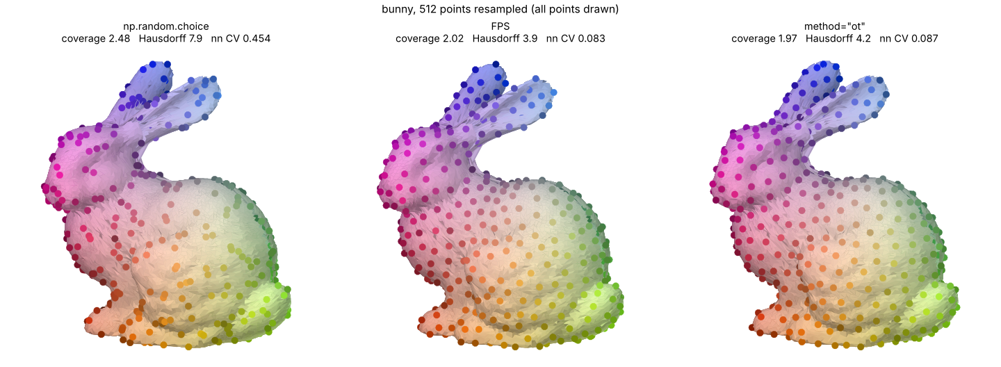
+fairly evenly spread over the surface. If method = "ot" is used, the initial resampling is
+optimised further using Optimal Transport.
 
 ```python
-sampler = flat.resample(n_points=512)   # n new points in total
+sampler = flat.resample(n_points=512, method="ot")   # n new points in total
 new = sampler.points                    # (512, 3)
 sampler.plot()                          # before / after
-other = flat.resample(n_points=512, seed=1)  # a new resampling, with different seed
 ```
+
 **To be honest:** if you only need a subset of the input points, farthest point sampling
-(FPS) are more uniform than flatpoints (figure below), this is mainly an exemple usecase to show how to use the images to transport properties (like good spatial repartition) from the simple unit square to an arbitrary surface.
+(FPS) is roughly as uniform as flatpoints (fps has slightly smaller worst case hole and 
+flatpoints.resample slitghly lower ot loss), this is mainly an example usecase to show how 
+to use the images to transport properties like good spatial repartition from the simple unit 
+square to an arbitrary surface.
 
 
 ![hyperuniform resampling: comparison](https://raw.githubusercontent.com/neighborhood-grid/flatpoints/main/plots/resampling/bunny_comparison.png)

{flatpoints-1.0.0 → flatpoints-1.1.0}/README.md

@@ -67,6 +67,7 @@ z = xyz[:, -1] #(N, *C) any data related to the point cloud, e.g. the z coordina
 # ==== Build the flat object ============
 
 flat = fp.Flat(xyz) # Apply the flattening processing of the surface
+# flat = fp.Flat(xyz, mesh=(vertices, triangles))  # giving your mesh as additional input (optional).
 
 # ==== Use it: pixels and images ========
 
@@ -113,16 +114,20 @@ cloud. So one can sample points in the unit square and transport them onto the s
 bilinear interpolation of the xyz image, (row, col) → xyz.
 
 By default, `flat.resample` uses a hyperuniform 2D seed (blue noise), so the new points are
-fairly evenly spread over the surface.
+fairly evenly spread over the surface. If method = "ot" is used, the initial resampling is
+optimised further using Optimal Transport.
 
 ```python
-sampler = flat.resample(n_points=512)   # n new points in total
+sampler = flat.resample(n_points=512, method="ot")   # n new points in total
 new = sampler.points                    # (512, 3)
 sampler.plot()                          # before / after
-other = flat.resample(n_points=512, seed=1)  # a new resampling, with different seed
 ```
+
 **To be honest:** if you only need a subset of the input points, farthest point sampling
-(FPS) are more uniform than flatpoints (figure below), this is mainly an exemple usecase to show how to use the images to transport properties (like good spatial repartition) from the simple unit square to an arbitrary surface.
+(FPS) is roughly as uniform as flatpoints (fps has slightly smaller worst case hole and 
+flatpoints.resample slitghly lower ot loss), this is mainly an example usecase to show how 
+to use the images to transport properties like good spatial repartition from the simple unit 
+square to an arbitrary surface.
 
 
 ![hyperuniform resampling: comparison](https://raw.githubusercontent.com/neighborhood-grid/flatpoints/main/plots/resampling/bunny_comparison.png)
@@ -202,4 +207,4 @@ The images rely on the rectangular conformal map of:
   year    = {2016},
   doi     = {10.1137/15M1049117}
 }
-```
+```

{flatpoints-1.0.0 → flatpoints-1.1.0}/pyproject.toml

@@ -4,7 +4,7 @@ build-backend = "setuptools.build_meta"
 
 [project]
 name = "flatpoints"
-version = "1.0.0"
+version = "1.1.0"
 description = "Flatten a point cloud into square images where neighbour pixels are neighbour points"
 readme = { file = "README.md", content-type = "text/markdown" }
 license = "MIT AND Apache-2.0"  # MIT, except src/flatpoints/rcm.py (Apache-2.0)

{flatpoints-1.0.0 → flatpoints-1.1.0}/src/flatpoints/__init__.py

@@ -5,4 +5,4 @@ from .main import Compressor, Flat, Resampler
 
 __all__ = ["Flat", "Resampler", "Compressor", "load", "datasets",
            "exemple_flat", "exemple_sampler", "exemple_compression"]
-__version__ = "1.0.0"
+__version__ = "1.1.0"

{flatpoints-1.0.0 → flatpoints-1.1.0}/src/flatpoints/main.py

@@ -9,7 +9,8 @@ from scipy.ndimage import gaussian_filter, map_coordinates
 from scipy.spatial import cKDTree
 
 from .core import conformal_uv, image_cells
-from .mesh import TRIM, closest_on_mesh, disk_cut, hemisphere_cut, poisson_mesh, submesh
+from .mesh import TRIM, closest_on_mesh, disk_cut, given_mesh, hemisphere_cut, poisson_mesh, submesh
+from .resampler import lloyd_ot
 from .utils import axes, fill_empty, Chart, Corners, Mesh, _window, _seeds, ON_SURFACE
 
 
@@ -53,6 +54,9 @@ class Flat(Viz):
 
     Args:
         points: (N, 3) points sampled on a surface.
+        mesh: optional mesh of the surface, used instead of the Poisson reconstruction:
+            (vertices (V, 3), triangles (F, 3)), or any object with `vertices` and
+            `faces` (or `triangles`), e.g. trimesh, open3d. The points are projected on it.
         single_face: True for an open surface (one image), False for a closed one (two
             images, the surface cut in left and right halves).
         normal_axis: "x", "y" or "z". Orients the images (rows follow z, or y if
@@ -73,17 +77,19 @@ class Flat(Viz):
         new = flat.resample(512).points     # (512, 3)
     """
 
-    def __init__(self, points, single_face=False, normal_axis="x", verbose=False):
+    def __init__(self, points, single_face=False, normal_axis="x", verbose=False, mesh=None):
         self.points = P = np.asarray(points, float)
         self.normal_axis, self.single_face = normal_axis, single_face
         normal, horiz, vert = axes(normal_axis)
 
         # 1. Mesh, cut into charts
+        if mesh is not None:
+            V, F = given_mesh(mesh)
+        else:
+            V, F = poisson_mesh(P, trim=TRIM if single_face else None)
         if single_face:
-            V, F = poisson_mesh(P, trim=TRIM)
             side = disk_cut(V, F)
         else:
-            V, F = poisson_mesh(P)
             side = hemisphere_cut(V, F, normal, np.median(P[:, normal]))
         self._mesh = Mesh(V, F, side)
         if verbose:
@@ -129,9 +135,9 @@ class Flat(Viz):
 
         self.corners = Corners(np.concatenate(pad_idxs), np.concatenate(pad_pixels))
 
-    def resample(self, n_points=512, seed=42, sigma=0.0):
+    def resample(self, n_points=512, seed=42, sigma=0.0, method="seed", n_iter=10):
         """`n_points` new points evenly spread on the surface, see `Resampler`."""
-        return Resampler(self, n_points, seed, sigma)
+        return Resampler(self, n_points, seed, sigma, method, n_iter)
 
     def compress(self, factor=0.8, method="auto"):
         """Compress the points, `factor` (e.g. 0.8) of the storage saved, with `method`
@@ -173,13 +179,15 @@ class Resampler:
         seed: int (shift of the default hyperuniform seed), (M, 2) points in [0, 1)^2, or
             {face name: (M, 2)}.
         sigma: Gaussian smoothing of the images before lifting, in pixels.
+        method: "seed" (the seed lifted to 3D) or "ot" (then `n_iter` Lloyd iterations of
+            optimal transport onto the input cloud, see `resampler.py`).
 
     Attributes:
         points: (n_points, 3); faces: (n_points,); pixels: (n_points, 3) float
         (face, row, col).
     """
 
-    def __init__(self, flat, n_points=512, seed=42, sigma=0.0):
+    def __init__(self, flat, n_points=512, seed=42, sigma=0.0, method="seed", n_iter=10):
         self.flat, self.n_points, self.sigma = flat, n_points, sigma
         names = ("main",) if flat.single_face else ("left", "right")
         if n_points < len(names):
@@ -210,6 +218,10 @@ class Resampler:
         self.points = np.concatenate(points)
         self.pixels = np.concatenate(pixels)
         self.faces = self.pixels[:, 0].astype(int)
+        if method == "ot":
+            self.points, self.pixels = lloyd_ot(flat, self.points, self.pixels, n_iter)
+        elif method != "seed":
+            raise ValueError('method must be "seed" or "ot"')
 
     def plot(self, ax=None, point_size=1.0, **kwargs):
         """Before (input cloud, left) / after (new points on its mesh, right), in 3D.

{flatpoints-1.0.0 → flatpoints-1.1.0}/src/flatpoints/mesh.py

@@ -37,6 +37,32 @@ def poisson_mesh(points, depth=POISSON_DEPTH, trim=None):
         spacing = tree.query(points, k=7)[0][:, 1:].mean(1)
         d, i = tree.query(np.asarray(mesh.vertices))
         mesh.remove_vertices_by_mask(d > trim * spacing[i])
+    return clean(mesh)
+
+
+def given_mesh(mesh):
+    """(V, F) of a mesh given by the user, in the standard format: (vertices (V, 3),
+    triangles (F, 3)), or any object with `vertices` and `faces` (or `triangles`), e.g.
+    trimesh, open3d. Cleaned like the Poisson mesh, duplicated vertices merged first."""
+    import open3d as o3d
+    if isinstance(mesh, (tuple, list)):
+        V, F = mesh
+    else:
+        V = mesh.vertices  # faces first: trimesh.triangles are (F, 3, 3) coordinates
+        F = mesh.faces if hasattr(mesh, "faces") else mesh.triangles
+    V, F = np.asarray(V, float), np.asarray(F)
+    if V.ndim != 2 or V.shape[1] != 3 or F.ndim != 2 or F.shape[1] != 3:
+        raise ValueError("mesh: (vertices (V, 3), triangles (F, 3)), got "
+                         f"{V.shape} and {F.shape}")
+    mesh = o3d.geometry.TriangleMesh(o3d.utility.Vector3dVector(V),
+                                     o3d.utility.Vector3iVector(F.astype(np.int32)))
+    mesh.remove_duplicated_vertices()
+    return clean(mesh)
+
+
+def clean(mesh):
+    """(V, F) of the open3d `mesh` without degenerate triangles nor non-manifold edges,
+    its largest piece only."""
     mesh.remove_degenerate_triangles()
     mesh.remove_non_manifold_edges()
     piece, sizes, _ = mesh.cluster_connected_triangles()

flatpoints-1.1.0/src/flatpoints/resampler.py

@@ -0,0 +1,79 @@
+"""`Resampler(..., method="ot")`: the seed, then Lloyd iterations of optimal transport.
+
+Each new point receives N / M input points (exact masses), by optimal transport between
+the points, with the true cost ||x - y||^2 in 3D, then moves to the barycentre of its input
+points. No mesh is used (it is only a reconstruction, it can miss thin parts): at the end,
+each barycentre (slightly inside the surface where it curves) is projected on the tangent
+plane of its nearest input point, fitted on the input points around it.
+
+The images make the transport sparse: an input point may only go to its K nearest new
+points on the images (N K pairs, instead of N M), and no farther than REACH times the
+spacing of the new points in 3D (across a tear, a candidate can be near on the image and
+far on the surface).
+
+The transport is solved by its dual (a power diagram): input point j goes to the
+candidate i minimising ||x_j - y_i||^2 - w_i, and the weight w_i rises if cell i has too
+few points, falls if it has too many. numpy only; the weights are kept from one Lloyd
+iteration to the next, so a few dual steps suffice. Cells hold N / M points up to a few.
+"""
+import numpy as np
+from scipy.spatial import cKDTree
+
+K = 8            # candidate new points of an input point, nearest on the images
+REACH = 2.0      # ... and closer than REACH x the spacing of the new points in 3D
+DUAL_STEPS = 30  # dual steps per Lloyd iteration
+DUAL_RATE = 1.2  # dual step, x the typical cost / (N / M)
+K_PLANE = 10     # input points fitting a tangent plane
+
+
+def lloyd_ot(flat, points, pixels, n_iter=10):
+    """`n_iter` Lloyd iterations of sparse optimal transport from the new `points` (M, 3),
+    at `pixels` (M, 3) float (face, row, col) on the images of `flat`. Faces do not change.
+    Returns (points (M, 3), pixels (M, 3) float (face, row, col))."""
+    P, ip = flat.points, flat.pixels
+    points = np.asarray(points, float).copy()
+    pixels = np.asarray(pixels, float).copy()
+    face = pixels[:, 0].astype(int)
+    weights = np.zeros(len(points))
+    for _ in range(n_iter):
+        reach2 = REACH ** 2 * np.median(cKDTree(points).query(points, k=2)[0][:, 1]) ** 2
+        for f in range(flat.n_faces):
+            J, I = np.flatnonzero(ip[:, 0] == f), np.flatnonzero(face == f)
+            if len(I) == 0:
+                continue
+            k = min(K, len(I))
+            _, nb = cKDTree(pixels[I, 1:]).query(ip[J, 1:].astype(float), k=k)
+            nb = nb.reshape(len(J), k)
+            cost = ((P[J, None, :] - points[I][nb]) ** 2).sum(-1)
+            far = cost > reach2
+            far[np.arange(len(J)), cost.argmin(1)] = False  # always one candidate
+            cost[far] = np.inf
+
+            # transport: dual ascent on the weights of the cells
+            share = len(J) / len(I)
+            rate = DUAL_RATE * np.median(cost.min(1)) / share
+            w = weights[I]
+            for _ in range(DUAL_STEPS):
+                owner = nb[np.arange(len(J)), np.argmin(cost - w[nb], 1)]
+                count = np.bincount(owner, minlength=len(I))
+                w += rate * (share - count)
+            weights[I] = w
+
+            # Lloyd: barycentre of each cell (an empty cell keeps its point)
+            full = np.flatnonzero(count)
+            for x, out, cols in ((P[J], points, slice(None)),
+                                 (ip[J, 1:].astype(float), pixels, slice(1, 3))):
+                sums = np.stack([np.bincount(owner, c, len(I)) for c in x.T], 1)
+                out[I[full], cols] = sums[full] / count[full, None]
+    return tangent_projection(P, points), pixels
+
+
+def tangent_projection(P, Q):
+    """`Q` (M, 3) projected on the tangent plane of their nearest point of `P`, fitted
+    (PCA) on its K_PLANE nearest points."""
+    tree = cKDTree(P)
+    _, i = tree.query(Q)
+    _, around = tree.query(P[i], k=min(K_PLANE, len(P)))
+    X = P[around] - P[around].mean(1, keepdims=True)
+    normal = np.linalg.eigh(np.einsum("mki,mkj->mij", X, X))[1][:, :, 0]
+    return Q - ((Q - P[i]) * normal).sum(1, keepdims=True) * normal

{flatpoints-1.0.0 → flatpoints-1.1.0}/src/flatpoints/viz.py

@@ -89,7 +89,7 @@ def plot_resampler(sampler, ax=None, point_size=1.0, light=0.45, radius=None):
         if len(mine):  # shade of a point: the one of the nearest quad
             _, near = cKDTree(_quads(g["xyz"]).mean(2).reshape(-1, 3)).query(mine)
             layers.append(disc_layer(mine @ proj.T, rgb(mine, flat.points),
-                                     shade.ravel()[near], radius, push=radius, sides=10))
+                                     shade.ravel()[near], radius, push=3 * radius, sides=10))
     render(ax, layers)
     return ax.figure
 

{flatpoints-1.0.0 → flatpoints-1.1.0}/src/flatpoints.egg-info/PKG-INFO

@@ -1,6 +1,6 @@
 Metadata-Version: 2.4
 Name: flatpoints
-Version: 1.0.0
+Version: 1.1.0
 Summary: Flatten a point cloud into square images where neighbour pixels are neighbour points
 Author: Armand de Cacqueray
 License-Expression: MIT AND Apache-2.0
@@ -112,6 +112,7 @@ z = xyz[:, -1] #(N, *C) any data related to the point cloud, e.g. the z coordina
 # ==== Build the flat object ============
 
 flat = fp.Flat(xyz) # Apply the flattening processing of the surface
+# flat = fp.Flat(xyz, mesh=(vertices, triangles))  # giving your mesh as additional input (optional).
 
 # ==== Use it: pixels and images ========
 
@@ -158,16 +159,20 @@ cloud. So one can sample points in the unit square and transport them onto the s
 bilinear interpolation of the xyz image, (row, col) → xyz.
 
 By default, `flat.resample` uses a hyperuniform 2D seed (blue noise), so the new points are
-fairly evenly spread over the surface.
+fairly evenly spread over the surface. If method = "ot" is used, the initial resampling is
+optimised further using Optimal Transport.
 
 ```python
-sampler = flat.resample(n_points=512)   # n new points in total
+sampler = flat.resample(n_points=512, method="ot")   # n new points in total
 new = sampler.points                    # (512, 3)
 sampler.plot()                          # before / after
-other = flat.resample(n_points=512, seed=1)  # a new resampling, with different seed
 ```
+
 **To be honest:** if you only need a subset of the input points, farthest point sampling
-(FPS) are more uniform than flatpoints (figure below), this is mainly an exemple usecase to show how to use the images to transport properties (like good spatial repartition) from the simple unit square to an arbitrary surface.
+(FPS) is roughly as uniform as flatpoints (fps has slightly smaller worst case hole and 
+flatpoints.resample slitghly lower ot loss), this is mainly an example usecase to show how 
+to use the images to transport properties like good spatial repartition from the simple unit 
+square to an arbitrary surface.
 
 
 ![hyperuniform resampling: comparison](https://raw.githubusercontent.com/neighborhood-grid/flatpoints/main/plots/resampling/bunny_comparison.png)

{flatpoints-1.0.0 → flatpoints-1.1.0}/src/flatpoints.egg-info/SOURCES.txt

@@ -12,6 +12,7 @@ src/flatpoints/examples.py
 src/flatpoints/main.py
 src/flatpoints/mesh.py
 src/flatpoints/rcm.py
+src/flatpoints/resampler.py
 src/flatpoints/utils.py
 src/flatpoints/viz.py
 src/flatpoints.egg-info/PKG-INFO

flatpoints-1.0.0/Method.md

@@ -1,49 +0,0 @@
-# Method
-
-flatpoints takes a point cloud sampled on a surface and returns one or two square images: each point of the cloud on its own pixel, neighbour pixels holding neighbour points.
-
-```
-points ──► mesh, cut into disks ──► map onto a square (conformal) ──► gridify (conformal to equal area) ──► image
-```
-
-This is the *geometry image* of Gu, Gortler & Hoppe (2002), with one difference: no
-resampling. The pixels are the input points themselves, so `flat.pixels` gives the exact
-point <-> pixel correspondence.
-
-## 1. Mesh and cut
-
-A square is a topological disk, so the surface must first be cut into disks, the faces.
-
-- **Mesh**: mesh the point cloud using screened Poisson reconstruction (open3d) 
-- **Cut**: a closed surface is split into two faces, left and right of the median along
-  `normal_axis`; an open surface is a single face. Faces grow triangle by triangle and
-  only accept triangles that keep them a disk, so handles and holes are left cut open.
-- **Points**: each point is projected onto the mesh and takes the face of its triangle.
-
-## 2. Conformal map
-
-Each face is mapped onto the unit square by a rectangular conformal map (Meng, Choi & Lui
-2016). Each point takes the uv_conformal of its projection on the mesh.
-
-## 3. Grid
-
-The points of each face are sorted onto an n x n grid by their uv_conformal (gridpoints). The resulting one to one matching
-```
-point -> pixel = face, row, column
-```
-is the final output of the flatpoints. Due to the one to one assignement, the flattening is by construction an area preserving transformation.
-
-## Limits
-
-- **Cuts**: points on either side of a cut are neighbours on the surface but not in the images. This apply to the left / right cut of the single_face = False pipeline, but also on further topological closedness of the surface (e.g. for a torus), which will also be cut.
-- **Tears**: the grid cannot follow the uv exactly, so a few adjacent pixels hold points
-  several spacings apart (2.7% beyond 3 spacings on the bunny).
-- **Meshing**: since flatpoints operate on point cloud with unkown surface, the overal precision of the flattening will depend on the quality of the meshing performed by open3d.
-
-## References
-
-X. Gu, S. J. Gortler and H. Hoppe, "Geometry Images", SIGGRAPH 2002.
-[hhoppe.com/proj/gim](https://hhoppe.com/proj/gim/)
-
-T. W. Meng, G. P.-T. Choi and L. M. Lui, "TEMPO: Feature-Endowed Teichmüller Extremal
-Mappings of Point Clouds", SIAM J. Imaging Sciences, 9(4), 2016.