data-availability 0.1.0__tar.gz → 0.3.1__tar.gz
This diff represents the content of publicly available package versions that have been released to one of the supported registries. The information contained in this diff is provided for informational purposes only and reflects changes between package versions as they appear in their respective public registries.
- data_availability-0.3.1/PKG-INFO +245 -0
- data_availability-0.3.1/README.md +224 -0
- {data_availability-0.1.0 → data_availability-0.3.1}/pyproject.toml +8 -6
- data_availability-0.3.1/src/data_availability/.cache/uv/.gitignore +1 -0
- data_availability-0.3.1/src/data_availability/.cache/uv/.lock +0 -0
- data_availability-0.3.1/src/data_availability/.cache/uv/CACHEDIR.TAG +1 -0
- data_availability-0.3.1/src/data_availability/.cache/uv/interpreter-v4/0de9bff94b993286/aa3e97e98ed0a440.msgpack +0 -0
- data_availability-0.3.1/src/data_availability/.cache/uv/sdists-v9/.git +0 -0
- data_availability-0.3.1/src/data_availability/.cache/uv/sdists-v9/.gitignore +0 -0
- {data_availability-0.1.0 → data_availability-0.3.1}/src/data_availability/__init__.py +40 -36
- data_availability-0.3.1/src/data_availability/availability.py +137 -0
- data_availability-0.3.1/src/data_availability/logger.py +163 -0
- {data_availability-0.1.0 → data_availability-0.3.1}/src/data_availability/plot.py +273 -74
- data_availability-0.3.1/src/data_availability/seismic/__init__.py +0 -0
- data_availability-0.3.1/src/data_availability/seismic/sds.py +217 -0
- data_availability-0.3.1/src/data_availability/seismic/seismic_availability.py +256 -0
- data_availability-0.3.1/src/data_availability/utils.py +54 -0
- data_availability-0.1.0/PKG-INFO +0 -137
- data_availability-0.1.0/README.md +0 -118
- data_availability-0.1.0/src/data_availability/availability.py +0 -89
- {data_availability-0.1.0 → data_availability-0.3.1}/src/data_availability/data.py +0 -0
|
@@ -0,0 +1,245 @@
|
|
|
1
|
+
Metadata-Version: 2.4
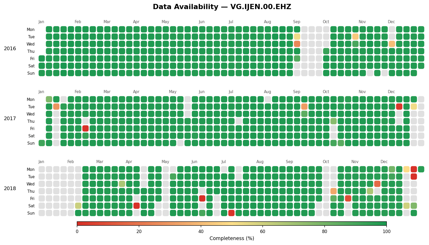
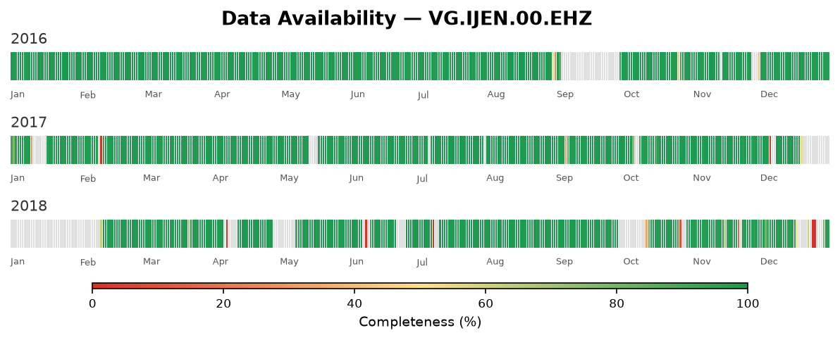
|
|
2
|
+
Name: data-availability
|
|
3
|
+
Version: 0.3.1
|
|
4
|
+
Summary: Plot data availability for seismic
|
|
5
|
+
Keywords: volcano,volcanology,seismic,data,plot,availability
|
|
6
|
+
Author: Martanto
|
|
7
|
+
Author-email: Martanto <martanto@live.com>
|
|
8
|
+
License-Expression: MIT
|
|
9
|
+
Classifier: Development Status :: 3 - Alpha
|
|
10
|
+
Classifier: Intended Audience :: Science/Research
|
|
11
|
+
Classifier: Operating System :: OS Independent
|
|
12
|
+
Classifier: Programming Language :: Python :: 3.11
|
|
13
|
+
Classifier: Programming Language :: Python :: 3.12
|
|
14
|
+
Requires-Dist: loguru>=0.7.3
|
|
15
|
+
Requires-Dist: matplotlib>=3.10.9
|
|
16
|
+
Requires-Dist: obspy>=1.5.0
|
|
17
|
+
Requires-Dist: openpyxl>=3.1.5
|
|
18
|
+
Requires-Dist: pandas>=3.0.2
|
|
19
|
+
Requires-Python: >=3.11
|
|
20
|
+
Description-Content-Type: text/markdown
|
|
21
|
+
|
|
22
|
+
# data-availability
|
|
23
|
+
|
|
24
|
+
[](https://pypi.org/project/data-availability/)
|
|
25
|
+
[](https://pypi.org/project/data-availability/)
|
|
26
|
+
[](https://pypi.org/project/data-availability/)
|
|
27
|
+
[](https://github.com/martanto/data-availability)
|
|
28
|
+
[](https://pepy.tech/projects/data-availability)
|
|
29
|
+
|
|
30
|
+
Calendar heatmaps and daily bar strips that show data completeness over time.
|
|
31
|
+
|
|
32
|
+
Use it to monitor instrument data quality or to track the availability of any time series. It returns a matplotlib `Figure` with one subplot per calendar year, with each day colored on a red-yellow-green gradient by its completeness.
|
|
33
|
+
|
|
34
|
+
**Input**: Excel (`.xlsx`/`.xls`) or CSV with `date` and `completeness` (0–100) columns.
|
|
35
|
+
**Output**: A `matplotlib.figure.Figure` — save or display as needed.
|
|
36
|
+
|
|
37
|
+
There are two kinds of figure:
|
|
38
|
+
|
|
39
|
+
- **`kind="calendar"`** (default): a GitHub contribution-style heatmap, with one tile per day on a Mon–Sun × week grid.
|
|
40
|
+
|
|
41
|
+
|
|
42
|
+
|
|
43
|
+
- **`kind="bar"`**: a status-page style strip, with one thin bar per day and month labels underneath.
|
|
44
|
+
|
|
45
|
+
|
|
46
|
+
|
|
47
|
+
## Installation
|
|
48
|
+
|
|
49
|
+
```bash
|
|
50
|
+
pip install data-availability
|
|
51
|
+
```
|
|
52
|
+
|
|
53
|
+
Or with [uv](https://docs.astral.sh/uv/):
|
|
54
|
+
|
|
55
|
+
```bash
|
|
56
|
+
uv add data-availability
|
|
57
|
+
```
|
|
58
|
+
|
|
59
|
+
## Quick start
|
|
60
|
+
|
|
61
|
+
### Fluent builder (recommended)
|
|
62
|
+
|
|
63
|
+
```python
|
|
64
|
+
import matplotlib.pyplot as plt
|
|
65
|
+
from data_availability import PlotAvailability
|
|
66
|
+
|
|
67
|
+
fig = (
|
|
68
|
+
PlotAvailability("data.xlsx")
|
|
69
|
+
.select(years="2023")
|
|
70
|
+
.plot(title="Sensor Uptime", tile_shape="squircle")
|
|
71
|
+
)
|
|
72
|
+
plt.savefig("availability.png", dpi=150, bbox_inches="tight")
|
|
73
|
+
|
|
74
|
+
# Same data as a daily bar strip
|
|
75
|
+
fig = (
|
|
76
|
+
PlotAvailability("data.xlsx")
|
|
77
|
+
.select(years=["2022", "2023"])
|
|
78
|
+
.plot(title="Sensor Uptime", kind="bar", fig_width=10)
|
|
79
|
+
)
|
|
80
|
+
fig.savefig("availability-bar.png", dpi=150, bbox_inches="tight")
|
|
81
|
+
```
|
|
82
|
+
|
|
83
|
+
### One-call helpers
|
|
84
|
+
|
|
85
|
+
```python
|
|
86
|
+
from data_availability import plot_from_file, plot_from_df
|
|
87
|
+
|
|
88
|
+
# From a file
|
|
89
|
+
fig = plot_from_file("data.csv", title="My Data")
|
|
90
|
+
|
|
91
|
+
# From a pre-loaded DataFrame
|
|
92
|
+
import pandas as pd
|
|
93
|
+
df = pd.read_csv("data.csv")
|
|
94
|
+
fig = plot_from_df(df, title="My Data")
|
|
95
|
+
```
|
|
96
|
+
|
|
97
|
+
### Seismic SDS data
|
|
98
|
+
|
|
99
|
+
```python
|
|
100
|
+
from data_availability import SeismicAvailability
|
|
101
|
+
|
|
102
|
+
sa = SeismicAvailability(
|
|
103
|
+
start_date="2023-01-01",
|
|
104
|
+
end_date="2023-12-31",
|
|
105
|
+
sds_dir="/data/sds",
|
|
106
|
+
station="IJEN",
|
|
107
|
+
channel="EHZ",
|
|
108
|
+
network="VG",
|
|
109
|
+
location="00",
|
|
110
|
+
n_jobs=4,
|
|
111
|
+
)
|
|
112
|
+
|
|
113
|
+
fig = sa.plot(title="IJEN EHZ Availability 2023")
|
|
114
|
+
fig.savefig("ijen_availability.png", dpi=150, bbox_inches="tight")
|
|
115
|
+
|
|
116
|
+
fig = sa.plot(title="IJEN EHZ Availability 2023", kind="bar")
|
|
117
|
+
|
|
118
|
+
# Optional: persist the per-day completeness DataFrame
|
|
119
|
+
sa.to_excel() # writes <NSLC>_<start>-<end>.xlsx into CWD
|
|
120
|
+
sa.to_excel("ijen.xlsx") # or pass an explicit path
|
|
121
|
+
records = sa.to_json() # or serialise to JSON records
|
|
122
|
+
```
|
|
123
|
+
|
|
124
|
+
> On Windows, wrap the call in `if __name__ == "__main__":` when using
|
|
125
|
+
> `n_jobs > 1` — Python's `spawn` start method requires it.
|
|
126
|
+
|
|
127
|
+
## API reference
|
|
128
|
+
|
|
129
|
+
### `PlotAvailability(filepath)`
|
|
130
|
+
|
|
131
|
+
Fluent builder class for Excel/CSV data.
|
|
132
|
+
|
|
133
|
+
```python
|
|
134
|
+
fig = (
|
|
135
|
+
PlotAvailability("data.xlsx")
|
|
136
|
+
.select(
|
|
137
|
+
date_column="date", # column name for dates
|
|
138
|
+
completeness_column="completeness", # column name for values (0–100)
|
|
139
|
+
years=["2022", "2023"], # filter to specific years (optional)
|
|
140
|
+
)
|
|
141
|
+
.plot(
|
|
142
|
+
title="Data Availability",
|
|
143
|
+
kind="calendar", # "calendar" (heatmap) or "bar" (daily strip)
|
|
144
|
+
hspace=None, # default: 0.2 calendar, 1.4 bar
|
|
145
|
+
figsize_per_year=None, # inches per year; default: 2.2 calendar, 1.2 bar
|
|
146
|
+
fig_width=20.0, # figure width in inches
|
|
147
|
+
missing_color="#e0e0e0", # days absent from the data
|
|
148
|
+
cbar_bottom=20, # px between last subplot and colorbar
|
|
149
|
+
cbar_height=10, # colorbar height in px
|
|
150
|
+
title_pad=40, # px between first subplot and title
|
|
151
|
+
tile_shape="square", # calendar only: "square" or "squircle"
|
|
152
|
+
tile_gap=0.9, # calendar only: tile size (< 1 adds gaps)
|
|
153
|
+
bar_gap=0.8, # bar only: bar width (< 1 adds gaps)
|
|
154
|
+
)
|
|
155
|
+
)
|
|
156
|
+
```
|
|
157
|
+
|
|
158
|
+
`tile_shape` and `tile_gap` are ignored when `kind="bar"`, and `bar_gap` is
|
|
159
|
+
ignored when `kind="calendar"`. Any other `kind` raises `ValueError`.
|
|
160
|
+
|
|
161
|
+
### `SeismicAvailability(...)`
|
|
162
|
+
|
|
163
|
+
Reads a SeisComP Data Structure (SDS) archive, computes per-day completeness,
|
|
164
|
+
and renders the heatmap. Supports parallel processing via `n_jobs`.
|
|
165
|
+
|
|
166
|
+
```python
|
|
167
|
+
sa = SeismicAvailability(
|
|
168
|
+
start_date="2023-01-01", # YYYY-MM-DD
|
|
169
|
+
end_date="2023-12-31", # YYYY-MM-DD (inclusive)
|
|
170
|
+
sds_dir="/data/sds", # root of the SDS archive
|
|
171
|
+
station="IJEN",
|
|
172
|
+
channel="EHZ",
|
|
173
|
+
network="VG",
|
|
174
|
+
location="00",
|
|
175
|
+
channel_type="D", # SDS data-type qualifier (default "D")
|
|
176
|
+
n_jobs=1, # parallel workers (default 1 = serial)
|
|
177
|
+
verbose=False,
|
|
178
|
+
)
|
|
179
|
+
|
|
180
|
+
sa.plot(title="IJEN EHZ") # returns a matplotlib Figure; accepts the same
|
|
181
|
+
# kwargs as PlotAvailability.plot() (title defaults to NSLC)
|
|
182
|
+
sa.get_df() # DataFrame: nslc, date, filepath, completeness
|
|
183
|
+
sa.to_json() # list of records
|
|
184
|
+
sa.to_excel(path=None) # write DataFrame to Excel; default filename in CWD
|
|
185
|
+
```
|
|
186
|
+
|
|
187
|
+
With `kind="calendar"`, `.plot()` drops zero-completeness days, so days
|
|
188
|
+
with no data render as `missing_color` (grey) instead of red at the bottom
|
|
189
|
+
of the colormap. With `kind="bar"`, those days are kept and render red, so
|
|
190
|
+
outages stand out in the strip. Call `.get_df()` for the unfiltered per-day
|
|
191
|
+
results.
|
|
192
|
+
|
|
193
|
+
### `plot_from_file(filepath, **kwargs)` / `plot_from_df(df, **kwargs)`
|
|
194
|
+
|
|
195
|
+
Functional alternatives that accept the same keyword arguments as `.plot()` (including `kind`) plus `date_column` and `completeness_column`.
|
|
196
|
+
|
|
197
|
+
These don't filter out zero-completeness rows, so those days render red in both kinds.
|
|
198
|
+
|
|
199
|
+
### `load_data(filepath, date_column, completeness_column)`
|
|
200
|
+
|
|
201
|
+
Load and normalize an Excel or CSV file into a DataFrame ready for plotting.
|
|
202
|
+
|
|
203
|
+
## Logging
|
|
204
|
+
|
|
205
|
+
A stderr console handler at `INFO` level is attached automatically on
|
|
206
|
+
import — you don't need to configure anything to see log output. Opt into
|
|
207
|
+
rotating daily file logs (general + errors) by calling `configure_logging`:
|
|
208
|
+
|
|
209
|
+
```python
|
|
210
|
+
from data_availability import configure_logging
|
|
211
|
+
|
|
212
|
+
configure_logging(log_dir="./logs", console_level="DEBUG")
|
|
213
|
+
```
|
|
214
|
+
|
|
215
|
+
The library never creates directories or writes files on import.
|
|
216
|
+
|
|
217
|
+
## Input format
|
|
218
|
+
|
|
219
|
+
| Column | Type | Notes |
|
|
220
|
+
|---|---|---|
|
|
221
|
+
| `date` | date string or datetime | parsed automatically |
|
|
222
|
+
| `completeness` | float | clipped to [0, 100]; strings replaced with NaN |
|
|
223
|
+
|
|
224
|
+
Column names are configurable via `date_column` / `completeness_column` parameters.
|
|
225
|
+
|
|
226
|
+
## Development
|
|
227
|
+
|
|
228
|
+
```bash
|
|
229
|
+
# Install with dev extras
|
|
230
|
+
uv sync --group dev
|
|
231
|
+
|
|
232
|
+
# Run the example (writes output.png and output-bar.png)
|
|
233
|
+
uv run main.py
|
|
234
|
+
|
|
235
|
+
# Lint and format
|
|
236
|
+
uv run ruff check --fix .
|
|
237
|
+
uv run ruff format .
|
|
238
|
+
|
|
239
|
+
# Type check
|
|
240
|
+
uv run ty check
|
|
241
|
+
```
|
|
242
|
+
|
|
243
|
+
## License
|
|
244
|
+
|
|
245
|
+
MIT © [Martanto](https://github.com/martanto)
|
|
@@ -0,0 +1,224 @@
|
|
|
1
|
+
# data-availability
|
|
2
|
+
|
|
3
|
+
[](https://pypi.org/project/data-availability/)
|
|
4
|
+
[](https://pypi.org/project/data-availability/)
|
|
5
|
+
[](https://pypi.org/project/data-availability/)
|
|
6
|
+
[](https://github.com/martanto/data-availability)
|
|
7
|
+
[](https://pepy.tech/projects/data-availability)
|
|
8
|
+
|
|
9
|
+
Calendar heatmaps and daily bar strips that show data completeness over time.
|
|
10
|
+
|
|
11
|
+
Use it to monitor instrument data quality or to track the availability of any time series. It returns a matplotlib `Figure` with one subplot per calendar year, with each day colored on a red-yellow-green gradient by its completeness.
|
|
12
|
+
|
|
13
|
+
**Input**: Excel (`.xlsx`/`.xls`) or CSV with `date` and `completeness` (0–100) columns.
|
|
14
|
+
**Output**: A `matplotlib.figure.Figure` — save or display as needed.
|
|
15
|
+
|
|
16
|
+
There are two kinds of figure:
|
|
17
|
+
|
|
18
|
+
- **`kind="calendar"`** (default): a GitHub contribution-style heatmap, with one tile per day on a Mon–Sun × week grid.
|
|
19
|
+
|
|
20
|
+

|
|
21
|
+
|
|
22
|
+
- **`kind="bar"`**: a status-page style strip, with one thin bar per day and month labels underneath.
|
|
23
|
+
|
|
24
|
+

|
|
25
|
+
|
|
26
|
+
## Installation
|
|
27
|
+
|
|
28
|
+
```bash
|
|
29
|
+
pip install data-availability
|
|
30
|
+
```
|
|
31
|
+
|
|
32
|
+
Or with [uv](https://docs.astral.sh/uv/):
|
|
33
|
+
|
|
34
|
+
```bash
|
|
35
|
+
uv add data-availability
|
|
36
|
+
```
|
|
37
|
+
|
|
38
|
+
## Quick start
|
|
39
|
+
|
|
40
|
+
### Fluent builder (recommended)
|
|
41
|
+
|
|
42
|
+
```python
|
|
43
|
+
import matplotlib.pyplot as plt
|
|
44
|
+
from data_availability import PlotAvailability
|
|
45
|
+
|
|
46
|
+
fig = (
|
|
47
|
+
PlotAvailability("data.xlsx")
|
|
48
|
+
.select(years="2023")
|
|
49
|
+
.plot(title="Sensor Uptime", tile_shape="squircle")
|
|
50
|
+
)
|
|
51
|
+
plt.savefig("availability.png", dpi=150, bbox_inches="tight")
|
|
52
|
+
|
|
53
|
+
# Same data as a daily bar strip
|
|
54
|
+
fig = (
|
|
55
|
+
PlotAvailability("data.xlsx")
|
|
56
|
+
.select(years=["2022", "2023"])
|
|
57
|
+
.plot(title="Sensor Uptime", kind="bar", fig_width=10)
|
|
58
|
+
)
|
|
59
|
+
fig.savefig("availability-bar.png", dpi=150, bbox_inches="tight")
|
|
60
|
+
```
|
|
61
|
+
|
|
62
|
+
### One-call helpers
|
|
63
|
+
|
|
64
|
+
```python
|
|
65
|
+
from data_availability import plot_from_file, plot_from_df
|
|
66
|
+
|
|
67
|
+
# From a file
|
|
68
|
+
fig = plot_from_file("data.csv", title="My Data")
|
|
69
|
+
|
|
70
|
+
# From a pre-loaded DataFrame
|
|
71
|
+
import pandas as pd
|
|
72
|
+
df = pd.read_csv("data.csv")
|
|
73
|
+
fig = plot_from_df(df, title="My Data")
|
|
74
|
+
```
|
|
75
|
+
|
|
76
|
+
### Seismic SDS data
|
|
77
|
+
|
|
78
|
+
```python
|
|
79
|
+
from data_availability import SeismicAvailability
|
|
80
|
+
|
|
81
|
+
sa = SeismicAvailability(
|
|
82
|
+
start_date="2023-01-01",
|
|
83
|
+
end_date="2023-12-31",
|
|
84
|
+
sds_dir="/data/sds",
|
|
85
|
+
station="IJEN",
|
|
86
|
+
channel="EHZ",
|
|
87
|
+
network="VG",
|
|
88
|
+
location="00",
|
|
89
|
+
n_jobs=4,
|
|
90
|
+
)
|
|
91
|
+
|
|
92
|
+
fig = sa.plot(title="IJEN EHZ Availability 2023")
|
|
93
|
+
fig.savefig("ijen_availability.png", dpi=150, bbox_inches="tight")
|
|
94
|
+
|
|
95
|
+
fig = sa.plot(title="IJEN EHZ Availability 2023", kind="bar")
|
|
96
|
+
|
|
97
|
+
# Optional: persist the per-day completeness DataFrame
|
|
98
|
+
sa.to_excel() # writes <NSLC>_<start>-<end>.xlsx into CWD
|
|
99
|
+
sa.to_excel("ijen.xlsx") # or pass an explicit path
|
|
100
|
+
records = sa.to_json() # or serialise to JSON records
|
|
101
|
+
```
|
|
102
|
+
|
|
103
|
+
> On Windows, wrap the call in `if __name__ == "__main__":` when using
|
|
104
|
+
> `n_jobs > 1` — Python's `spawn` start method requires it.
|
|
105
|
+
|
|
106
|
+
## API reference
|
|
107
|
+
|
|
108
|
+
### `PlotAvailability(filepath)`
|
|
109
|
+
|
|
110
|
+
Fluent builder class for Excel/CSV data.
|
|
111
|
+
|
|
112
|
+
```python
|
|
113
|
+
fig = (
|
|
114
|
+
PlotAvailability("data.xlsx")
|
|
115
|
+
.select(
|
|
116
|
+
date_column="date", # column name for dates
|
|
117
|
+
completeness_column="completeness", # column name for values (0–100)
|
|
118
|
+
years=["2022", "2023"], # filter to specific years (optional)
|
|
119
|
+
)
|
|
120
|
+
.plot(
|
|
121
|
+
title="Data Availability",
|
|
122
|
+
kind="calendar", # "calendar" (heatmap) or "bar" (daily strip)
|
|
123
|
+
hspace=None, # default: 0.2 calendar, 1.4 bar
|
|
124
|
+
figsize_per_year=None, # inches per year; default: 2.2 calendar, 1.2 bar
|
|
125
|
+
fig_width=20.0, # figure width in inches
|
|
126
|
+
missing_color="#e0e0e0", # days absent from the data
|
|
127
|
+
cbar_bottom=20, # px between last subplot and colorbar
|
|
128
|
+
cbar_height=10, # colorbar height in px
|
|
129
|
+
title_pad=40, # px between first subplot and title
|
|
130
|
+
tile_shape="square", # calendar only: "square" or "squircle"
|
|
131
|
+
tile_gap=0.9, # calendar only: tile size (< 1 adds gaps)
|
|
132
|
+
bar_gap=0.8, # bar only: bar width (< 1 adds gaps)
|
|
133
|
+
)
|
|
134
|
+
)
|
|
135
|
+
```
|
|
136
|
+
|
|
137
|
+
`tile_shape` and `tile_gap` are ignored when `kind="bar"`, and `bar_gap` is
|
|
138
|
+
ignored when `kind="calendar"`. Any other `kind` raises `ValueError`.
|
|
139
|
+
|
|
140
|
+
### `SeismicAvailability(...)`
|
|
141
|
+
|
|
142
|
+
Reads a SeisComP Data Structure (SDS) archive, computes per-day completeness,
|
|
143
|
+
and renders the heatmap. Supports parallel processing via `n_jobs`.
|
|
144
|
+
|
|
145
|
+
```python
|
|
146
|
+
sa = SeismicAvailability(
|
|
147
|
+
start_date="2023-01-01", # YYYY-MM-DD
|
|
148
|
+
end_date="2023-12-31", # YYYY-MM-DD (inclusive)
|
|
149
|
+
sds_dir="/data/sds", # root of the SDS archive
|
|
150
|
+
station="IJEN",
|
|
151
|
+
channel="EHZ",
|
|
152
|
+
network="VG",
|
|
153
|
+
location="00",
|
|
154
|
+
channel_type="D", # SDS data-type qualifier (default "D")
|
|
155
|
+
n_jobs=1, # parallel workers (default 1 = serial)
|
|
156
|
+
verbose=False,
|
|
157
|
+
)
|
|
158
|
+
|
|
159
|
+
sa.plot(title="IJEN EHZ") # returns a matplotlib Figure; accepts the same
|
|
160
|
+
# kwargs as PlotAvailability.plot() (title defaults to NSLC)
|
|
161
|
+
sa.get_df() # DataFrame: nslc, date, filepath, completeness
|
|
162
|
+
sa.to_json() # list of records
|
|
163
|
+
sa.to_excel(path=None) # write DataFrame to Excel; default filename in CWD
|
|
164
|
+
```
|
|
165
|
+
|
|
166
|
+
With `kind="calendar"`, `.plot()` drops zero-completeness days, so days
|
|
167
|
+
with no data render as `missing_color` (grey) instead of red at the bottom
|
|
168
|
+
of the colormap. With `kind="bar"`, those days are kept and render red, so
|
|
169
|
+
outages stand out in the strip. Call `.get_df()` for the unfiltered per-day
|
|
170
|
+
results.
|
|
171
|
+
|
|
172
|
+
### `plot_from_file(filepath, **kwargs)` / `plot_from_df(df, **kwargs)`
|
|
173
|
+
|
|
174
|
+
Functional alternatives that accept the same keyword arguments as `.plot()` (including `kind`) plus `date_column` and `completeness_column`.
|
|
175
|
+
|
|
176
|
+
These don't filter out zero-completeness rows, so those days render red in both kinds.
|
|
177
|
+
|
|
178
|
+
### `load_data(filepath, date_column, completeness_column)`
|
|
179
|
+
|
|
180
|
+
Load and normalize an Excel or CSV file into a DataFrame ready for plotting.
|
|
181
|
+
|
|
182
|
+
## Logging
|
|
183
|
+
|
|
184
|
+
A stderr console handler at `INFO` level is attached automatically on
|
|
185
|
+
import — you don't need to configure anything to see log output. Opt into
|
|
186
|
+
rotating daily file logs (general + errors) by calling `configure_logging`:
|
|
187
|
+
|
|
188
|
+
```python
|
|
189
|
+
from data_availability import configure_logging
|
|
190
|
+
|
|
191
|
+
configure_logging(log_dir="./logs", console_level="DEBUG")
|
|
192
|
+
```
|
|
193
|
+
|
|
194
|
+
The library never creates directories or writes files on import.
|
|
195
|
+
|
|
196
|
+
## Input format
|
|
197
|
+
|
|
198
|
+
| Column | Type | Notes |
|
|
199
|
+
|---|---|---|
|
|
200
|
+
| `date` | date string or datetime | parsed automatically |
|
|
201
|
+
| `completeness` | float | clipped to [0, 100]; strings replaced with NaN |
|
|
202
|
+
|
|
203
|
+
Column names are configurable via `date_column` / `completeness_column` parameters.
|
|
204
|
+
|
|
205
|
+
## Development
|
|
206
|
+
|
|
207
|
+
```bash
|
|
208
|
+
# Install with dev extras
|
|
209
|
+
uv sync --group dev
|
|
210
|
+
|
|
211
|
+
# Run the example (writes output.png and output-bar.png)
|
|
212
|
+
uv run main.py
|
|
213
|
+
|
|
214
|
+
# Lint and format
|
|
215
|
+
uv run ruff check --fix .
|
|
216
|
+
uv run ruff format .
|
|
217
|
+
|
|
218
|
+
# Type check
|
|
219
|
+
uv run ty check
|
|
220
|
+
```
|
|
221
|
+
|
|
222
|
+
## License
|
|
223
|
+
|
|
224
|
+
MIT © [Martanto](https://github.com/martanto)
|
|
@@ -4,7 +4,7 @@ build-backend = "uv_build"
|
|
|
4
4
|
|
|
5
5
|
[project]
|
|
6
6
|
name = "data-availability"
|
|
7
|
-
version = "0.1
|
|
7
|
+
version = "0.3.1"
|
|
8
8
|
authors = [
|
|
9
9
|
{name = "Martanto", email = "martanto@live.com"},
|
|
10
10
|
]
|
|
@@ -14,7 +14,9 @@ license = "MIT"
|
|
|
14
14
|
keywords = ["volcano", "volcanology", "seismic", "data", "plot", "availability"]
|
|
15
15
|
requires-python = ">=3.11"
|
|
16
16
|
dependencies = [
|
|
17
|
+
"loguru>=0.7.3",
|
|
17
18
|
"matplotlib>=3.10.9",
|
|
19
|
+
"obspy>=1.5.0",
|
|
18
20
|
"openpyxl>=3.1.5",
|
|
19
21
|
"pandas>=3.0.2",
|
|
20
22
|
]
|
|
@@ -28,11 +30,11 @@ classifiers = [
|
|
|
28
30
|
|
|
29
31
|
[dependency-groups]
|
|
30
32
|
dev = [
|
|
31
|
-
"ipykernel
|
|
32
|
-
"notebook
|
|
33
|
-
"pandas-stubs
|
|
34
|
-
"ruff
|
|
35
|
-
"ty
|
|
33
|
+
"ipykernel",
|
|
34
|
+
"notebook",
|
|
35
|
+
"pandas-stubs",
|
|
36
|
+
"ruff",
|
|
37
|
+
"ty",
|
|
36
38
|
]
|
|
37
39
|
|
|
38
40
|
[tool.uv]
|
|
@@ -0,0 +1 @@
|
|
|
1
|
+
*
|
|
File without changes
|
|
@@ -0,0 +1 @@
|
|
|
1
|
+
Signature: 8a477f597d28d172789f06886806bc55
|
|
Binary file
|
|
File without changes
|
|
File without changes
|
|
@@ -1,36 +1,40 @@
|
|
|
1
|
-
"""data-availability: GitHub-style calendar heatmaps for data completeness.
|
|
2
|
-
|
|
3
|
-
Generates matplotlib figures showing data completeness over time, one subplot
|
|
4
|
-
per calendar year, color-coded on a red-yellow-green gradient.
|
|
5
|
-
|
|
6
|
-
Example:
|
|
7
|
-
>>> from data_availability import plot_from_file
|
|
8
|
-
>>> fig = plot_from_file("data.csv", title="Sensor Uptime")
|
|
9
|
-
>>> fig.savefig("availability.png", dpi=150)
|
|
10
|
-
"""
|
|
11
|
-
|
|
12
|
-
from importlib.metadata import version
|
|
13
|
-
|
|
14
|
-
from data_availability.data import load_data
|
|
15
|
-
from data_availability.plot import plot_from_df, plot_from_file
|
|
16
|
-
from data_availability.
|
|
17
|
-
|
|
18
|
-
|
|
19
|
-
|
|
20
|
-
|
|
21
|
-
|
|
22
|
-
|
|
23
|
-
|
|
24
|
-
|
|
25
|
-
|
|
26
|
-
|
|
27
|
-
|
|
28
|
-
|
|
29
|
-
"
|
|
30
|
-
"
|
|
31
|
-
"
|
|
32
|
-
"
|
|
33
|
-
"
|
|
34
|
-
"
|
|
35
|
-
"
|
|
36
|
-
|
|
1
|
+
"""data-availability: GitHub-style calendar heatmaps for data completeness.
|
|
2
|
+
|
|
3
|
+
Generates matplotlib figures showing data completeness over time, one subplot
|
|
4
|
+
per calendar year, color-coded on a red-yellow-green gradient.
|
|
5
|
+
|
|
6
|
+
Example:
|
|
7
|
+
>>> from data_availability import plot_from_file
|
|
8
|
+
>>> fig = plot_from_file("data.csv", title="Sensor Uptime")
|
|
9
|
+
>>> fig.savefig("availability.png", dpi=150)
|
|
10
|
+
"""
|
|
11
|
+
|
|
12
|
+
from importlib.metadata import version
|
|
13
|
+
|
|
14
|
+
from data_availability.data import load_data
|
|
15
|
+
from data_availability.plot import plot_from_df, plot_from_file
|
|
16
|
+
from data_availability.logger import configure_logging
|
|
17
|
+
from data_availability.availability import PlotAvailability
|
|
18
|
+
from data_availability.seismic.seismic_availability import SeismicAvailability
|
|
19
|
+
|
|
20
|
+
|
|
21
|
+
__version__ = version("data-availability")
|
|
22
|
+
__author__ = "Martanto"
|
|
23
|
+
__author_email__ = "martanto@live.com"
|
|
24
|
+
__license__ = "MIT"
|
|
25
|
+
__copyright__ = "Copyright (c) 2026, Martanto"
|
|
26
|
+
__url__ = "https://github.com/martanto/data-availability"
|
|
27
|
+
|
|
28
|
+
__all__ = [
|
|
29
|
+
"__version__",
|
|
30
|
+
"__author__",
|
|
31
|
+
"__author_email__",
|
|
32
|
+
"__license__",
|
|
33
|
+
"__copyright__",
|
|
34
|
+
"PlotAvailability",
|
|
35
|
+
"SeismicAvailability",
|
|
36
|
+
"configure_logging",
|
|
37
|
+
"load_data",
|
|
38
|
+
"plot_from_df",
|
|
39
|
+
"plot_from_file",
|
|
40
|
+
]
|