data-availability 0.1.0__tar.gz
This diff represents the content of publicly available package versions that have been released to one of the supported registries. The information contained in this diff is provided for informational purposes only and reflects changes between package versions as they appear in their respective public registries.
- data_availability-0.1.0/PKG-INFO +137 -0
- data_availability-0.1.0/README.md +118 -0
- data_availability-0.1.0/pyproject.toml +39 -0
- data_availability-0.1.0/src/data_availability/__init__.py +36 -0
- data_availability-0.1.0/src/data_availability/availability.py +89 -0
- data_availability-0.1.0/src/data_availability/data.py +72 -0
- data_availability-0.1.0/src/data_availability/plot.py +320 -0
|
@@ -0,0 +1,137 @@
|
|
|
1
|
+
Metadata-Version: 2.4
|
|
2
|
+
Name: data-availability
|
|
3
|
+
Version: 0.1.0
|
|
4
|
+
Summary: Plot data availability for seismic
|
|
5
|
+
Keywords: volcano,volcanology,seismic,data,plot,availability
|
|
6
|
+
Author: Martanto
|
|
7
|
+
Author-email: Martanto <martanto@live.com>
|
|
8
|
+
License-Expression: MIT
|
|
9
|
+
Classifier: Development Status :: 3 - Alpha
|
|
10
|
+
Classifier: Intended Audience :: Science/Research
|
|
11
|
+
Classifier: Operating System :: OS Independent
|
|
12
|
+
Classifier: Programming Language :: Python :: 3.11
|
|
13
|
+
Classifier: Programming Language :: Python :: 3.12
|
|
14
|
+
Requires-Dist: matplotlib>=3.10.9
|
|
15
|
+
Requires-Dist: openpyxl>=3.1.5
|
|
16
|
+
Requires-Dist: pandas>=3.0.2
|
|
17
|
+
Requires-Python: >=3.11
|
|
18
|
+
Description-Content-Type: text/markdown
|
|
19
|
+
|
|
20
|
+
# data-availability
|
|
21
|
+
|
|
22
|
+
GitHub contribution-style calendar heatmaps for data completeness over time.
|
|
23
|
+
|
|
24
|
+
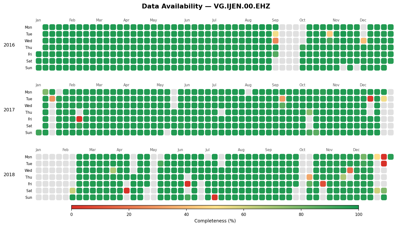
Useful for monitoring instrument data quality or any time-series availability tracking. Generates a matplotlib `Figure` with one subplot per calendar year, each day rendered as a color-coded tile on a red-yellow-green gradient.
|
|
25
|
+
|
|
26
|
+
**Input**: Excel (`.xlsx`/`.xls`) or CSV with `date` and `completeness` (0–100) columns.
|
|
27
|
+
**Output**: A `matplotlib.figure.Figure` — save or display as needed.
|
|
28
|
+
|
|
29
|
+
|
|
30
|
+
|
|
31
|
+
## Installation
|
|
32
|
+
|
|
33
|
+
```bash
|
|
34
|
+
pip install data-availability
|
|
35
|
+
```
|
|
36
|
+
|
|
37
|
+
Or with [uv](https://docs.astral.sh/uv/):
|
|
38
|
+
|
|
39
|
+
```bash
|
|
40
|
+
uv add data-availability
|
|
41
|
+
```
|
|
42
|
+
|
|
43
|
+
## Quick start
|
|
44
|
+
|
|
45
|
+
### Fluent builder (recommended)
|
|
46
|
+
|
|
47
|
+
```python
|
|
48
|
+
import matplotlib.pyplot as plt
|
|
49
|
+
from data_availability import PlotAvailability
|
|
50
|
+
|
|
51
|
+
fig = (
|
|
52
|
+
PlotAvailability("data.xlsx")
|
|
53
|
+
.load_data(years="2023")
|
|
54
|
+
.plot_availability(title="Sensor Uptime", tile_shape="squircle")
|
|
55
|
+
)
|
|
56
|
+
plt.savefig("availability.png", dpi=150, bbox_inches="tight")
|
|
57
|
+
```
|
|
58
|
+
|
|
59
|
+
### One-call helpers
|
|
60
|
+
|
|
61
|
+
```python
|
|
62
|
+
from data_availability import plot_from_file, plot_from_df
|
|
63
|
+
|
|
64
|
+
# From a file
|
|
65
|
+
fig = plot_from_file("data.csv", title="My Data")
|
|
66
|
+
|
|
67
|
+
# From a pre-loaded DataFrame
|
|
68
|
+
import pandas as pd
|
|
69
|
+
df = pd.read_csv("data.csv")
|
|
70
|
+
fig = plot_from_df(df, title="My Data")
|
|
71
|
+
```
|
|
72
|
+
|
|
73
|
+
## API reference
|
|
74
|
+
|
|
75
|
+
### `PlotAvailability(filepath)`
|
|
76
|
+
|
|
77
|
+
Fluent builder class.
|
|
78
|
+
|
|
79
|
+
```python
|
|
80
|
+
fig = (
|
|
81
|
+
PlotAvailability("data.xlsx")
|
|
82
|
+
.load_data(
|
|
83
|
+
date_column="date", # column name for dates
|
|
84
|
+
completeness_column="completeness", # column name for values (0–100)
|
|
85
|
+
years=["2022", "2023"], # filter to specific years (optional)
|
|
86
|
+
)
|
|
87
|
+
.plot_availability(
|
|
88
|
+
title="Data Availability",
|
|
89
|
+
tile_shape="square", # "square" or "squircle"
|
|
90
|
+
hspace=0.2,
|
|
91
|
+
figsize_per_year=2.2,
|
|
92
|
+
missing_color="#e0e0e0",
|
|
93
|
+
cbar_bottom=20,
|
|
94
|
+
cbar_height=10,
|
|
95
|
+
tile_gap=0.9,
|
|
96
|
+
title_pad=40,
|
|
97
|
+
)
|
|
98
|
+
)
|
|
99
|
+
```
|
|
100
|
+
|
|
101
|
+
### `plot_from_file(filepath, **kwargs)` / `plot_from_df(df, **kwargs)`
|
|
102
|
+
|
|
103
|
+
Functional alternatives that accept the same keyword arguments as `.plot_availability()` plus `date_column` and `completeness_column`.
|
|
104
|
+
|
|
105
|
+
### `load_data(filepath, date_column, completeness_column)`
|
|
106
|
+
|
|
107
|
+
Load and normalize an Excel or CSV file into a DataFrame ready for plotting.
|
|
108
|
+
|
|
109
|
+
## Input format
|
|
110
|
+
|
|
111
|
+
| Column | Type | Notes |
|
|
112
|
+
|---|---|---|
|
|
113
|
+
| `date` | date string or datetime | parsed automatically |
|
|
114
|
+
| `completeness` | float | clipped to [0, 100]; strings replaced with NaN |
|
|
115
|
+
|
|
116
|
+
Column names are configurable via `date_column` / `completeness_column` parameters.
|
|
117
|
+
|
|
118
|
+
## Development
|
|
119
|
+
|
|
120
|
+
```bash
|
|
121
|
+
# Install with dev extras
|
|
122
|
+
uv sync --group dev
|
|
123
|
+
|
|
124
|
+
# Run the example
|
|
125
|
+
uv run main.py
|
|
126
|
+
|
|
127
|
+
# Lint and format
|
|
128
|
+
uv run ruff check --fix .
|
|
129
|
+
uv run ruff format .
|
|
130
|
+
|
|
131
|
+
# Type check
|
|
132
|
+
uv run ty check
|
|
133
|
+
```
|
|
134
|
+
|
|
135
|
+
## License
|
|
136
|
+
|
|
137
|
+
MIT © [Martanto](https://github.com/martanto)
|
|
@@ -0,0 +1,118 @@
|
|
|
1
|
+
# data-availability
|
|
2
|
+
|
|
3
|
+
GitHub contribution-style calendar heatmaps for data completeness over time.
|
|
4
|
+
|
|
5
|
+
Useful for monitoring instrument data quality or any time-series availability tracking. Generates a matplotlib `Figure` with one subplot per calendar year, each day rendered as a color-coded tile on a red-yellow-green gradient.
|
|
6
|
+
|
|
7
|
+
**Input**: Excel (`.xlsx`/`.xls`) or CSV with `date` and `completeness` (0–100) columns.
|
|
8
|
+
**Output**: A `matplotlib.figure.Figure` — save or display as needed.
|
|
9
|
+
|
|
10
|
+

|
|
11
|
+
|
|
12
|
+
## Installation
|
|
13
|
+
|
|
14
|
+
```bash
|
|
15
|
+
pip install data-availability
|
|
16
|
+
```
|
|
17
|
+
|
|
18
|
+
Or with [uv](https://docs.astral.sh/uv/):
|
|
19
|
+
|
|
20
|
+
```bash
|
|
21
|
+
uv add data-availability
|
|
22
|
+
```
|
|
23
|
+
|
|
24
|
+
## Quick start
|
|
25
|
+
|
|
26
|
+
### Fluent builder (recommended)
|
|
27
|
+
|
|
28
|
+
```python
|
|
29
|
+
import matplotlib.pyplot as plt
|
|
30
|
+
from data_availability import PlotAvailability
|
|
31
|
+
|
|
32
|
+
fig = (
|
|
33
|
+
PlotAvailability("data.xlsx")
|
|
34
|
+
.load_data(years="2023")
|
|
35
|
+
.plot_availability(title="Sensor Uptime", tile_shape="squircle")
|
|
36
|
+
)
|
|
37
|
+
plt.savefig("availability.png", dpi=150, bbox_inches="tight")
|
|
38
|
+
```
|
|
39
|
+
|
|
40
|
+
### One-call helpers
|
|
41
|
+
|
|
42
|
+
```python
|
|
43
|
+
from data_availability import plot_from_file, plot_from_df
|
|
44
|
+
|
|
45
|
+
# From a file
|
|
46
|
+
fig = plot_from_file("data.csv", title="My Data")
|
|
47
|
+
|
|
48
|
+
# From a pre-loaded DataFrame
|
|
49
|
+
import pandas as pd
|
|
50
|
+
df = pd.read_csv("data.csv")
|
|
51
|
+
fig = plot_from_df(df, title="My Data")
|
|
52
|
+
```
|
|
53
|
+
|
|
54
|
+
## API reference
|
|
55
|
+
|
|
56
|
+
### `PlotAvailability(filepath)`
|
|
57
|
+
|
|
58
|
+
Fluent builder class.
|
|
59
|
+
|
|
60
|
+
```python
|
|
61
|
+
fig = (
|
|
62
|
+
PlotAvailability("data.xlsx")
|
|
63
|
+
.load_data(
|
|
64
|
+
date_column="date", # column name for dates
|
|
65
|
+
completeness_column="completeness", # column name for values (0–100)
|
|
66
|
+
years=["2022", "2023"], # filter to specific years (optional)
|
|
67
|
+
)
|
|
68
|
+
.plot_availability(
|
|
69
|
+
title="Data Availability",
|
|
70
|
+
tile_shape="square", # "square" or "squircle"
|
|
71
|
+
hspace=0.2,
|
|
72
|
+
figsize_per_year=2.2,
|
|
73
|
+
missing_color="#e0e0e0",
|
|
74
|
+
cbar_bottom=20,
|
|
75
|
+
cbar_height=10,
|
|
76
|
+
tile_gap=0.9,
|
|
77
|
+
title_pad=40,
|
|
78
|
+
)
|
|
79
|
+
)
|
|
80
|
+
```
|
|
81
|
+
|
|
82
|
+
### `plot_from_file(filepath, **kwargs)` / `plot_from_df(df, **kwargs)`
|
|
83
|
+
|
|
84
|
+
Functional alternatives that accept the same keyword arguments as `.plot_availability()` plus `date_column` and `completeness_column`.
|
|
85
|
+
|
|
86
|
+
### `load_data(filepath, date_column, completeness_column)`
|
|
87
|
+
|
|
88
|
+
Load and normalize an Excel or CSV file into a DataFrame ready for plotting.
|
|
89
|
+
|
|
90
|
+
## Input format
|
|
91
|
+
|
|
92
|
+
| Column | Type | Notes |
|
|
93
|
+
|---|---|---|
|
|
94
|
+
| `date` | date string or datetime | parsed automatically |
|
|
95
|
+
| `completeness` | float | clipped to [0, 100]; strings replaced with NaN |
|
|
96
|
+
|
|
97
|
+
Column names are configurable via `date_column` / `completeness_column` parameters.
|
|
98
|
+
|
|
99
|
+
## Development
|
|
100
|
+
|
|
101
|
+
```bash
|
|
102
|
+
# Install with dev extras
|
|
103
|
+
uv sync --group dev
|
|
104
|
+
|
|
105
|
+
# Run the example
|
|
106
|
+
uv run main.py
|
|
107
|
+
|
|
108
|
+
# Lint and format
|
|
109
|
+
uv run ruff check --fix .
|
|
110
|
+
uv run ruff format .
|
|
111
|
+
|
|
112
|
+
# Type check
|
|
113
|
+
uv run ty check
|
|
114
|
+
```
|
|
115
|
+
|
|
116
|
+
## License
|
|
117
|
+
|
|
118
|
+
MIT © [Martanto](https://github.com/martanto)
|
|
@@ -0,0 +1,39 @@
|
|
|
1
|
+
[build-system]
|
|
2
|
+
requires = ["uv_build<0.12"]
|
|
3
|
+
build-backend = "uv_build"
|
|
4
|
+
|
|
5
|
+
[project]
|
|
6
|
+
name = "data-availability"
|
|
7
|
+
version = "0.1.0"
|
|
8
|
+
authors = [
|
|
9
|
+
{name = "Martanto", email = "martanto@live.com"},
|
|
10
|
+
]
|
|
11
|
+
description = "Plot data availability for seismic"
|
|
12
|
+
readme = "README.md"
|
|
13
|
+
license = "MIT"
|
|
14
|
+
keywords = ["volcano", "volcanology", "seismic", "data", "plot", "availability"]
|
|
15
|
+
requires-python = ">=3.11"
|
|
16
|
+
dependencies = [
|
|
17
|
+
"matplotlib>=3.10.9",
|
|
18
|
+
"openpyxl>=3.1.5",
|
|
19
|
+
"pandas>=3.0.2",
|
|
20
|
+
]
|
|
21
|
+
classifiers = [
|
|
22
|
+
"Development Status :: 3 - Alpha",
|
|
23
|
+
"Intended Audience :: Science/Research",
|
|
24
|
+
"Operating System :: OS Independent",
|
|
25
|
+
"Programming Language :: Python :: 3.11",
|
|
26
|
+
"Programming Language :: Python :: 3.12",
|
|
27
|
+
]
|
|
28
|
+
|
|
29
|
+
[dependency-groups]
|
|
30
|
+
dev = [
|
|
31
|
+
"ipykernel>=7.2.0",
|
|
32
|
+
"notebook>=7.5.6",
|
|
33
|
+
"pandas-stubs==3.0.0.260204",
|
|
34
|
+
"ruff>=0.15.12",
|
|
35
|
+
"ty>=0.0.34",
|
|
36
|
+
]
|
|
37
|
+
|
|
38
|
+
[tool.uv]
|
|
39
|
+
cache-dir = "./.cache/uv"
|
|
@@ -0,0 +1,36 @@
|
|
|
1
|
+
"""data-availability: GitHub-style calendar heatmaps for data completeness.
|
|
2
|
+
|
|
3
|
+
Generates matplotlib figures showing data completeness over time, one subplot
|
|
4
|
+
per calendar year, color-coded on a red-yellow-green gradient.
|
|
5
|
+
|
|
6
|
+
Example:
|
|
7
|
+
>>> from data_availability import plot_from_file
|
|
8
|
+
>>> fig = plot_from_file("data.csv", title="Sensor Uptime")
|
|
9
|
+
>>> fig.savefig("availability.png", dpi=150)
|
|
10
|
+
"""
|
|
11
|
+
|
|
12
|
+
from importlib.metadata import version
|
|
13
|
+
|
|
14
|
+
from data_availability.data import load_data
|
|
15
|
+
from data_availability.plot import plot_from_df, plot_from_file
|
|
16
|
+
from data_availability.availability import PlotAvailability
|
|
17
|
+
|
|
18
|
+
|
|
19
|
+
__version__ = version("data-availability")
|
|
20
|
+
__author__ = "Martanto"
|
|
21
|
+
__author_email__ = "martanto@live.com"
|
|
22
|
+
__license__ = "MIT"
|
|
23
|
+
__copyright__ = "Copyright (c) 2026, Martanto"
|
|
24
|
+
__url__ = "https://github.com/martanto/data-availability"
|
|
25
|
+
|
|
26
|
+
__all__ = [
|
|
27
|
+
"__version__",
|
|
28
|
+
"__author__",
|
|
29
|
+
"__author_email__",
|
|
30
|
+
"__license__",
|
|
31
|
+
"__copyright__",
|
|
32
|
+
"PlotAvailability",
|
|
33
|
+
"load_data",
|
|
34
|
+
"plot_from_df",
|
|
35
|
+
"plot_from_file",
|
|
36
|
+
]
|
|
@@ -0,0 +1,89 @@
|
|
|
1
|
+
from __future__ import annotations
|
|
2
|
+
|
|
3
|
+
from typing import Literal
|
|
4
|
+
from pathlib import Path
|
|
5
|
+
|
|
6
|
+
import pandas as pd
|
|
7
|
+
import matplotlib.pyplot as plt
|
|
8
|
+
|
|
9
|
+
from data_availability.data import load_data
|
|
10
|
+
from data_availability.plot import plot_from_df as _plot_from_df
|
|
11
|
+
|
|
12
|
+
|
|
13
|
+
class PlotAvailability:
|
|
14
|
+
def __init__(self, filepath: str | Path) -> None:
|
|
15
|
+
self._filepath = Path(filepath)
|
|
16
|
+
self._df: pd.DataFrame | None = None
|
|
17
|
+
self._date_column: str = "date"
|
|
18
|
+
self._completeness_column: str = "completeness"
|
|
19
|
+
|
|
20
|
+
def load_data(
|
|
21
|
+
self,
|
|
22
|
+
date_column: str = "date",
|
|
23
|
+
completeness_column: str = "completeness",
|
|
24
|
+
years: str | list[str] | None = None,
|
|
25
|
+
) -> PlotAvailability:
|
|
26
|
+
self._date_column = date_column
|
|
27
|
+
self._completeness_column = completeness_column
|
|
28
|
+
self._df = load_data(self._filepath, date_column, completeness_column)
|
|
29
|
+
if years is not None:
|
|
30
|
+
selected = [str(y) for y in ([years] if isinstance(years, str) else years)]
|
|
31
|
+
mask = self._df[date_column].dt.year.astype(str).isin(selected)
|
|
32
|
+
self._df = self._df[mask].reset_index(drop=True)
|
|
33
|
+
if isinstance(self._df, pd.DataFrame) and self._df.empty:
|
|
34
|
+
raise ValueError(
|
|
35
|
+
f"No data found for the specified year(s): {selected}."
|
|
36
|
+
)
|
|
37
|
+
return self
|
|
38
|
+
|
|
39
|
+
def plot_availability(
|
|
40
|
+
self,
|
|
41
|
+
title: str = "Data Availability",
|
|
42
|
+
hspace: float = 0.2,
|
|
43
|
+
cbar_bottom: int = 20,
|
|
44
|
+
cbar_height: int = 10,
|
|
45
|
+
tile_gap: float = 0.9,
|
|
46
|
+
figsize_per_year: float = 2.2,
|
|
47
|
+
missing_color: str = "#e0e0e0",
|
|
48
|
+
tile_shape: Literal["square", "squircle"] = "square",
|
|
49
|
+
title_pad: int = 40,
|
|
50
|
+
) -> plt.Figure:
|
|
51
|
+
"""Build a GitHub-style calendar heatmap of data completeness over time.
|
|
52
|
+
|
|
53
|
+
Args:
|
|
54
|
+
title: Figure super-title rendered above all subplots.
|
|
55
|
+
hspace: Vertical spacing between year subplots.
|
|
56
|
+
cbar_bottom: Gap in pixels between the bottom edge of the last subplot
|
|
57
|
+
and the top of the colorbar.
|
|
58
|
+
cbar_height: Height of the colorbar in pixels.
|
|
59
|
+
tile_gap: Side length of each day tile (values < 1 add whitespace
|
|
60
|
+
between tiles).
|
|
61
|
+
figsize_per_year: Figure height in inches allocated per year subplot.
|
|
62
|
+
missing_color: Color used for calendar days absent from the input data.
|
|
63
|
+
tile_shape: Shape of each day tile. ``"square"`` draws plain rectangles;
|
|
64
|
+
``"squircle"`` draws rectangles with rounded corners.
|
|
65
|
+
title_pad: Gap in pixels between the top of the last subplot and the
|
|
66
|
+
figure super-title.
|
|
67
|
+
|
|
68
|
+
Returns:
|
|
69
|
+
A :class:`matplotlib.figure.Figure` containing the heatmap.
|
|
70
|
+
|
|
71
|
+
Raises:
|
|
72
|
+
RuntimeError: If :meth:`load_data` has not been called first.
|
|
73
|
+
"""
|
|
74
|
+
if self._df is None:
|
|
75
|
+
raise RuntimeError("Call .load_data() before .plot_availability().")
|
|
76
|
+
return _plot_from_df(
|
|
77
|
+
self._df,
|
|
78
|
+
title=title,
|
|
79
|
+
date_column=self._date_column,
|
|
80
|
+
completeness_column=self._completeness_column,
|
|
81
|
+
hspace=hspace,
|
|
82
|
+
cbar_bottom=cbar_bottom,
|
|
83
|
+
cbar_height=cbar_height,
|
|
84
|
+
tile_gap=tile_gap,
|
|
85
|
+
figsize_per_year=figsize_per_year,
|
|
86
|
+
missing_color=missing_color,
|
|
87
|
+
tile_shape=tile_shape,
|
|
88
|
+
title_pad=title_pad,
|
|
89
|
+
)
|
|
@@ -0,0 +1,72 @@
|
|
|
1
|
+
import warnings
|
|
2
|
+
from pathlib import Path
|
|
3
|
+
|
|
4
|
+
import numpy as np
|
|
5
|
+
import pandas as pd
|
|
6
|
+
|
|
7
|
+
|
|
8
|
+
def load_data(
|
|
9
|
+
filepath: str | Path,
|
|
10
|
+
date_column: str = "date",
|
|
11
|
+
completeness_column: str = "completeness",
|
|
12
|
+
) -> pd.DataFrame:
|
|
13
|
+
"""Load and normalize availability data from an Excel or CSV file.
|
|
14
|
+
|
|
15
|
+
Reads a file containing ``date`` and ``completeness`` columns, parses
|
|
16
|
+
dates, clips completeness values to the range [0, 100], and returns the
|
|
17
|
+
result sorted by date.
|
|
18
|
+
|
|
19
|
+
Args:
|
|
20
|
+
filepath: Path to an ``.xlsx``, ``.xls``, or ``.csv`` file.
|
|
21
|
+
date_column: Name of the column to use as the date index. Defaults to
|
|
22
|
+
``"date"``.
|
|
23
|
+
completeness_column: Name of the column to use as completeness values.
|
|
24
|
+
Defaults to ``"completeness"``.
|
|
25
|
+
|
|
26
|
+
Returns:
|
|
27
|
+
A DataFrame with the selected date column (datetime64, time normalized
|
|
28
|
+
to midnight) and completeness column (float, 0–100), sorted ascending
|
|
29
|
+
by date with a reset integer index.
|
|
30
|
+
|
|
31
|
+
Raises:
|
|
32
|
+
FileNotFoundError: If ``filepath`` does not exist.
|
|
33
|
+
KeyError: If the file is missing the specified date or completeness column.
|
|
34
|
+
ValueError: If ``date`` values cannot be parsed as dates.
|
|
35
|
+
"""
|
|
36
|
+
path = Path(filepath)
|
|
37
|
+
if path.suffix in (".xlsx", ".xls"):
|
|
38
|
+
df = pd.read_excel(path)
|
|
39
|
+
else:
|
|
40
|
+
df = pd.read_csv(path)
|
|
41
|
+
|
|
42
|
+
missing = [
|
|
43
|
+
c for c in (date_column, completeness_column) if c not in df.columns.tolist()
|
|
44
|
+
]
|
|
45
|
+
if missing:
|
|
46
|
+
raise KeyError(f"Column(s) not found in file: {missing}")
|
|
47
|
+
|
|
48
|
+
df = df[[date_column, completeness_column]].copy()
|
|
49
|
+
|
|
50
|
+
df[date_column] = pd.to_datetime(df[date_column]).dt.normalize()
|
|
51
|
+
if not isinstance(
|
|
52
|
+
df[date_column].dtype, pd.DatetimeTZDtype
|
|
53
|
+
) and not pd.api.types.is_datetime64_any_dtype(df[date_column]):
|
|
54
|
+
raise ValueError(
|
|
55
|
+
f"Column '{date_column}' could not be parsed as DatetimeIndex."
|
|
56
|
+
)
|
|
57
|
+
|
|
58
|
+
string_mask = df[completeness_column].apply(lambda x: isinstance(x, str))
|
|
59
|
+
if string_mask.any():
|
|
60
|
+
n = string_mask.sum()
|
|
61
|
+
warnings.warn(
|
|
62
|
+
f"Column '{completeness_column}' contains {n} string value(s); replacing with NaN.",
|
|
63
|
+
UserWarning,
|
|
64
|
+
stacklevel=2,
|
|
65
|
+
)
|
|
66
|
+
df.loc[string_mask, completeness_column] = np.nan
|
|
67
|
+
|
|
68
|
+
df[completeness_column] = pd.to_numeric(
|
|
69
|
+
df[completeness_column], errors="coerce"
|
|
70
|
+
).clip(0, 100)
|
|
71
|
+
|
|
72
|
+
return df.sort_values(date_column).reset_index(drop=True)
|
|
@@ -0,0 +1,320 @@
|
|
|
1
|
+
from typing import Literal
|
|
2
|
+
from pathlib import Path
|
|
3
|
+
|
|
4
|
+
import numpy as np
|
|
5
|
+
import pandas as pd
|
|
6
|
+
import matplotlib.colors as mcolors
|
|
7
|
+
import matplotlib.pyplot as plt
|
|
8
|
+
import matplotlib.patches as mpatches
|
|
9
|
+
|
|
10
|
+
from data_availability.data import load_data
|
|
11
|
+
|
|
12
|
+
|
|
13
|
+
def _build_figure(
|
|
14
|
+
df: pd.DataFrame,
|
|
15
|
+
title: str,
|
|
16
|
+
date_column: str,
|
|
17
|
+
completeness_column: str,
|
|
18
|
+
hspace: float,
|
|
19
|
+
cbar_bottom: int,
|
|
20
|
+
cbar_height: int,
|
|
21
|
+
tile_gap: float,
|
|
22
|
+
figsize_per_year: float,
|
|
23
|
+
missing_color: str,
|
|
24
|
+
tile_shape: Literal["square", "squircle"],
|
|
25
|
+
title_pad: int,
|
|
26
|
+
) -> plt.Figure:
|
|
27
|
+
"""Render a GitHub-style calendar heatmap from a pre-validated DataFrame.
|
|
28
|
+
|
|
29
|
+
Internal helper called by :func:`plot_from_file` and :func:`plot_from_df`.
|
|
30
|
+
Creates one subplot per calendar year in ``df``, draws day tiles on a
|
|
31
|
+
Mon–Sun × week grid, attaches a horizontal colorbar below the last subplot,
|
|
32
|
+
and places a super-title above the first.
|
|
33
|
+
|
|
34
|
+
Args:
|
|
35
|
+
df: DataFrame with a datetime ``date_column`` and a numeric
|
|
36
|
+
``completeness_column`` (0–100), sorted ascending by date.
|
|
37
|
+
title: Figure super-title rendered above all subplots.
|
|
38
|
+
date_column: Name of the datetime column in ``df``.
|
|
39
|
+
completeness_column: Name of the numeric completeness column (0–100).
|
|
40
|
+
hspace: Vertical spacing between year subplots, passed to
|
|
41
|
+
``Figure.subplots_adjust``.
|
|
42
|
+
cbar_bottom: Gap in pixels between the bottom edge of the last subplot
|
|
43
|
+
and the top of the colorbar.
|
|
44
|
+
cbar_height: Height of the colorbar in pixels.
|
|
45
|
+
tile_gap: Side length of each day tile; values less than 1 add
|
|
46
|
+
whitespace between tiles.
|
|
47
|
+
figsize_per_year: Figure height in inches allocated per year subplot.
|
|
48
|
+
Total figure height is ``n_years * figsize_per_year``.
|
|
49
|
+
missing_color: Hex or named color for calendar days absent from
|
|
50
|
+
``df``.
|
|
51
|
+
tile_shape: ``"square"`` draws plain rectangles; ``"squircle"`` draws
|
|
52
|
+
rectangles with rounded corners.
|
|
53
|
+
title_pad: Gap in pixels between the top of the first subplot and the
|
|
54
|
+
figure super-title.
|
|
55
|
+
|
|
56
|
+
Returns:
|
|
57
|
+
A :class:`matplotlib.figure.Figure` containing the heatmap.
|
|
58
|
+
"""
|
|
59
|
+
years = sorted(df[date_column].dt.year.unique())
|
|
60
|
+
n_years = len(years)
|
|
61
|
+
|
|
62
|
+
fig, axes = plt.subplots(n_years, 1, figsize=(20, n_years * figsize_per_year))
|
|
63
|
+
if n_years == 1:
|
|
64
|
+
axes = [axes]
|
|
65
|
+
|
|
66
|
+
cmap = mcolors.LinearSegmentedColormap.from_list(
|
|
67
|
+
"rg", ["#d73027", "#fee08b", "#1a9850"]
|
|
68
|
+
)
|
|
69
|
+
norm = mcolors.Normalize(vmin=0, vmax=100)
|
|
70
|
+
|
|
71
|
+
day_labels = ["Mon", "Tue", "Wed", "Thu", "Fri", "Sat", "Sun"]
|
|
72
|
+
|
|
73
|
+
for ax, year in zip(axes, years, strict=True):
|
|
74
|
+
year_dates = pd.date_range(f"{year}-01-01", f"{year}-12-31", freq="D")
|
|
75
|
+
year_df = df[df[date_column].dt.year == year].set_index(date_column)[
|
|
76
|
+
completeness_column
|
|
77
|
+
]
|
|
78
|
+
|
|
79
|
+
# Build a 7-row (weekday) x 53-col (week) grid
|
|
80
|
+
grid = np.full((7, 53), np.nan)
|
|
81
|
+
has_data = np.zeros((7, 53), dtype=bool)
|
|
82
|
+
|
|
83
|
+
for date in year_dates:
|
|
84
|
+
# GitHub-style: week col starts from the week of Jan 1
|
|
85
|
+
day_of_year = date.day_of_year - 1 # 0-indexed
|
|
86
|
+
# week column: offset by weekday of Jan 1
|
|
87
|
+
jan1_weekday = pd.Timestamp(f"{year}-01-01").weekday() # Mon=0
|
|
88
|
+
col = (day_of_year + jan1_weekday) // 7
|
|
89
|
+
row = date.weekday() # Mon=0, Sun=6
|
|
90
|
+
has_data[row, col] = True
|
|
91
|
+
if date in year_df.index:
|
|
92
|
+
grid[row, col] = year_df[date]
|
|
93
|
+
else:
|
|
94
|
+
grid[row, col] = np.nan # missing = will render grey
|
|
95
|
+
|
|
96
|
+
# Draw tiles
|
|
97
|
+
rounding = tile_gap * 0.3
|
|
98
|
+
for col in range(53):
|
|
99
|
+
for row in range(7):
|
|
100
|
+
if not has_data[row, col]:
|
|
101
|
+
continue
|
|
102
|
+
val = grid[row, col]
|
|
103
|
+
color = missing_color if np.isnan(val) else cmap(norm(val))
|
|
104
|
+
if tile_shape == "squircle":
|
|
105
|
+
patch = mpatches.FancyBboxPatch(
|
|
106
|
+
(col, 6 - row),
|
|
107
|
+
tile_gap,
|
|
108
|
+
tile_gap,
|
|
109
|
+
boxstyle=f"round,pad=0,rounding_size={rounding}",
|
|
110
|
+
facecolor=color,
|
|
111
|
+
edgecolor="white",
|
|
112
|
+
linewidth=0.5,
|
|
113
|
+
)
|
|
114
|
+
else:
|
|
115
|
+
patch = mpatches.Rectangle(
|
|
116
|
+
(col, 6 - row),
|
|
117
|
+
tile_gap,
|
|
118
|
+
tile_gap,
|
|
119
|
+
facecolor=color,
|
|
120
|
+
edgecolor="white",
|
|
121
|
+
linewidth=0.5,
|
|
122
|
+
)
|
|
123
|
+
ax.add_patch(patch)
|
|
124
|
+
|
|
125
|
+
# Month label positions
|
|
126
|
+
month_starts = {}
|
|
127
|
+
for date in year_dates:
|
|
128
|
+
if date.day == 1:
|
|
129
|
+
jan1_weekday = pd.Timestamp(f"{year}-01-01").weekday()
|
|
130
|
+
day_of_year = date.day_of_year - 1
|
|
131
|
+
col = (day_of_year + jan1_weekday) // 7
|
|
132
|
+
month_starts[date.strftime("%b")] = col
|
|
133
|
+
|
|
134
|
+
for month, col in month_starts.items():
|
|
135
|
+
ax.text(
|
|
136
|
+
col + 0.4,
|
|
137
|
+
7.2,
|
|
138
|
+
month,
|
|
139
|
+
ha="center",
|
|
140
|
+
va="bottom",
|
|
141
|
+
fontsize=7,
|
|
142
|
+
color="#555",
|
|
143
|
+
)
|
|
144
|
+
|
|
145
|
+
ax.set_xlim(0, 53)
|
|
146
|
+
ax.set_ylim(-0.2, 7.8)
|
|
147
|
+
ax.set_aspect("equal")
|
|
148
|
+
ax.set_yticks([6 - r + tile_gap / 2 for r in range(7)])
|
|
149
|
+
ax.set_yticklabels(day_labels, fontsize=7)
|
|
150
|
+
ax.set_xticks([])
|
|
151
|
+
ax.set_ylabel(str(year), fontsize=9, rotation=0, labelpad=30, va="center")
|
|
152
|
+
ax.set_frame_on(False)
|
|
153
|
+
ax.tick_params(left=False)
|
|
154
|
+
|
|
155
|
+
fig.subplots_adjust(hspace=hspace)
|
|
156
|
+
|
|
157
|
+
# Get the bounding box of the last subplot to anchor the colorbar tightly below it
|
|
158
|
+
fig.canvas.draw()
|
|
159
|
+
last_ax = axes[-1]
|
|
160
|
+
first_ax = axes[0]
|
|
161
|
+
pos_last = last_ax.get_position()
|
|
162
|
+
pos_first = first_ax.get_position()
|
|
163
|
+
|
|
164
|
+
cbar_width = (pos_last.x1 - pos_last.x0) * 0.8
|
|
165
|
+
cbar_left = pos_last.x0 + (pos_last.x1 - pos_last.x0) * 0.1
|
|
166
|
+
fig_height_px = fig.get_size_inches()[1] * fig.dpi
|
|
167
|
+
cbar_height_fraction = cbar_height / fig_height_px
|
|
168
|
+
cbar_bottom_fraction = cbar_bottom / fig_height_px
|
|
169
|
+
cbar_ax = fig.add_axes(
|
|
170
|
+
[
|
|
171
|
+
cbar_left,
|
|
172
|
+
pos_last.y0 - cbar_bottom_fraction,
|
|
173
|
+
cbar_width,
|
|
174
|
+
cbar_height_fraction,
|
|
175
|
+
]
|
|
176
|
+
)
|
|
177
|
+
|
|
178
|
+
sm = plt.cm.ScalarMappable(cmap=cmap, norm=norm)
|
|
179
|
+
sm.set_array([])
|
|
180
|
+
cbar = fig.colorbar(sm, cax=cbar_ax, orientation="horizontal")
|
|
181
|
+
cbar.set_label("Completeness (%)", fontsize=9)
|
|
182
|
+
cbar.ax.tick_params(labelsize=8)
|
|
183
|
+
|
|
184
|
+
title_pad_fraction = title_pad / fig_height_px
|
|
185
|
+
fig.suptitle(title, fontsize=13, fontweight="bold", y=pos_first.y1 + title_pad_fraction)
|
|
186
|
+
|
|
187
|
+
return fig
|
|
188
|
+
|
|
189
|
+
|
|
190
|
+
def plot_from_file(
|
|
191
|
+
filepath: str | Path,
|
|
192
|
+
title: str = "Data Availability",
|
|
193
|
+
date_column: str = "date",
|
|
194
|
+
completeness_column: str = "completeness",
|
|
195
|
+
hspace: float = 0.2,
|
|
196
|
+
cbar_bottom: int = 20,
|
|
197
|
+
cbar_height: int = 10,
|
|
198
|
+
tile_gap: float = 0.9,
|
|
199
|
+
figsize_per_year: float = 2.2,
|
|
200
|
+
missing_color: str = "#e0e0e0",
|
|
201
|
+
tile_shape: Literal["square", "squircle"] = "square",
|
|
202
|
+
title_pad: int = 40,
|
|
203
|
+
) -> plt.Figure:
|
|
204
|
+
"""Build a GitHub-style calendar heatmap of data completeness from a file.
|
|
205
|
+
|
|
206
|
+
Loads data from an Excel or CSV file and delegates to
|
|
207
|
+
:func:`plot_from_df`. Creates one subplot per calendar year, with each day
|
|
208
|
+
rendered as a colored tile on a Mon–Sun × week grid. Tiles are color-coded
|
|
209
|
+
on a red-yellow-green gradient; days absent from the dataset are rendered
|
|
210
|
+
in ``missing_color``. A horizontal colorbar is placed below the last
|
|
211
|
+
subplot and a super-title above the first.
|
|
212
|
+
|
|
213
|
+
Args:
|
|
214
|
+
filepath: Path to an ``.xlsx``, ``.xls``, or ``.csv`` file accepted by
|
|
215
|
+
:func:`~data_availability.data.load_data`.
|
|
216
|
+
title: Figure super-title rendered above all subplots.
|
|
217
|
+
date_column: Name of the datetime column in the file.
|
|
218
|
+
completeness_column: Name of the numeric completeness column (0–100).
|
|
219
|
+
hspace: Vertical spacing between year subplots, passed to
|
|
220
|
+
``Figure.subplots_adjust``.
|
|
221
|
+
cbar_bottom: Gap in pixels between the bottom edge of the last subplot
|
|
222
|
+
and the top of the colorbar.
|
|
223
|
+
cbar_height: Height of the colorbar in pixels.
|
|
224
|
+
tile_gap: Side length of each day tile; values less than 1 add
|
|
225
|
+
whitespace between tiles.
|
|
226
|
+
figsize_per_year: Figure height in inches allocated per year subplot.
|
|
227
|
+
Total figure height is ``n_years * figsize_per_year``.
|
|
228
|
+
missing_color: Hex or named color for calendar days absent from the
|
|
229
|
+
input data.
|
|
230
|
+
tile_shape: ``"square"`` draws plain rectangles; ``"squircle"`` draws
|
|
231
|
+
rectangles with rounded corners.
|
|
232
|
+
title_pad: Gap in pixels between the top of the first subplot and the
|
|
233
|
+
figure super-title.
|
|
234
|
+
|
|
235
|
+
Returns:
|
|
236
|
+
A :class:`matplotlib.figure.Figure` containing the heatmap. The figure
|
|
237
|
+
is not saved or displayed; call ``fig.savefig()`` or ``plt.show()``
|
|
238
|
+
afterwards.
|
|
239
|
+
"""
|
|
240
|
+
df = load_data(
|
|
241
|
+
filepath, date_column=date_column, completeness_column=completeness_column
|
|
242
|
+
)
|
|
243
|
+
return _build_figure(
|
|
244
|
+
df,
|
|
245
|
+
title=title,
|
|
246
|
+
date_column=date_column,
|
|
247
|
+
completeness_column=completeness_column,
|
|
248
|
+
hspace=hspace,
|
|
249
|
+
cbar_bottom=cbar_bottom,
|
|
250
|
+
cbar_height=cbar_height,
|
|
251
|
+
tile_gap=tile_gap,
|
|
252
|
+
figsize_per_year=figsize_per_year,
|
|
253
|
+
missing_color=missing_color,
|
|
254
|
+
tile_shape=tile_shape,
|
|
255
|
+
title_pad=title_pad,
|
|
256
|
+
)
|
|
257
|
+
|
|
258
|
+
|
|
259
|
+
def plot_from_df(
|
|
260
|
+
df: pd.DataFrame,
|
|
261
|
+
title: str = "Data Availability",
|
|
262
|
+
date_column: str = "date",
|
|
263
|
+
completeness_column: str = "completeness",
|
|
264
|
+
hspace: float = 0.2,
|
|
265
|
+
cbar_bottom: int = 20,
|
|
266
|
+
cbar_height: int = 10,
|
|
267
|
+
tile_gap: float = 0.9,
|
|
268
|
+
figsize_per_year: float = 2.2,
|
|
269
|
+
missing_color: str = "#e0e0e0",
|
|
270
|
+
tile_shape: Literal["square", "squircle"] = "square",
|
|
271
|
+
title_pad: int = 40,
|
|
272
|
+
) -> plt.Figure:
|
|
273
|
+
"""Build a GitHub-style calendar heatmap from an in-memory DataFrame.
|
|
274
|
+
|
|
275
|
+
Accepts a pre-loaded :class:`~pandas.DataFrame` instead of a file path.
|
|
276
|
+
Useful when data has already been loaded and optionally filtered before
|
|
277
|
+
plotting. For file-based access see :func:`plot_from_file`.
|
|
278
|
+
|
|
279
|
+
Args:
|
|
280
|
+
df: DataFrame with a datetime ``date_column`` and a numeric
|
|
281
|
+
``completeness_column`` (0–100), as returned by
|
|
282
|
+
:func:`~data_availability.data.load_data`.
|
|
283
|
+
title: Figure super-title rendered above all subplots.
|
|
284
|
+
date_column: Name of the datetime column in ``df``.
|
|
285
|
+
completeness_column: Name of the numeric completeness column (0–100).
|
|
286
|
+
hspace: Vertical spacing between year subplots, passed to
|
|
287
|
+
``Figure.subplots_adjust``.
|
|
288
|
+
cbar_bottom: Gap in pixels between the bottom edge of the last subplot
|
|
289
|
+
and the top of the colorbar.
|
|
290
|
+
cbar_height: Height of the colorbar in pixels.
|
|
291
|
+
tile_gap: Side length of each day tile; values less than 1 add
|
|
292
|
+
whitespace between tiles.
|
|
293
|
+
figsize_per_year: Figure height in inches allocated per year subplot.
|
|
294
|
+
Total figure height is ``n_years * figsize_per_year``.
|
|
295
|
+
missing_color: Hex or named color for calendar days absent from
|
|
296
|
+
``df``.
|
|
297
|
+
tile_shape: ``"square"`` draws plain rectangles; ``"squircle"`` draws
|
|
298
|
+
rectangles with rounded corners.
|
|
299
|
+
title_pad: Gap in pixels between the top of the first subplot and the
|
|
300
|
+
figure super-title.
|
|
301
|
+
|
|
302
|
+
Returns:
|
|
303
|
+
A :class:`matplotlib.figure.Figure` containing the heatmap. The figure
|
|
304
|
+
is not saved or displayed; call ``fig.savefig()`` or ``plt.show()``
|
|
305
|
+
afterwards.
|
|
306
|
+
"""
|
|
307
|
+
return _build_figure(
|
|
308
|
+
df,
|
|
309
|
+
title=title,
|
|
310
|
+
date_column=date_column,
|
|
311
|
+
completeness_column=completeness_column,
|
|
312
|
+
hspace=hspace,
|
|
313
|
+
cbar_bottom=cbar_bottom,
|
|
314
|
+
cbar_height=cbar_height,
|
|
315
|
+
tile_gap=tile_gap,
|
|
316
|
+
figsize_per_year=figsize_per_year,
|
|
317
|
+
missing_color=missing_color,
|
|
318
|
+
tile_shape=tile_shape,
|
|
319
|
+
title_pad=title_pad,
|
|
320
|
+
)
|