catagg 0.1.0.dev0__tar.gz → 0.1.0.dev1__tar.gz
This diff represents the content of publicly available package versions that have been released to one of the supported registries. The information contained in this diff is provided for informational purposes only and reflects changes between package versions as they appear in their respective public registries.
- catagg-0.1.0.dev1/.gitignore +24 -0
- catagg-0.1.0.dev1/CHANGELOG.md +95 -0
- {catagg-0.1.0.dev0 → catagg-0.1.0.dev1}/PKG-INFO +25 -25
- {catagg-0.1.0.dev0 → catagg-0.1.0.dev1}/README.md +19 -23
- catagg-0.1.0.dev1/docs/financial.md +92 -0
- catagg-0.1.0.dev1/docs/img/gross_vs_net_oep.png +0 -0
- {catagg-0.1.0.dev0 → catagg-0.1.0.dev1}/docs/index.md +1 -0
- catagg-0.1.0.dev1/docs/metrics.md +148 -0
- catagg-0.1.0.dev1/docs/simulation.md +188 -0
- catagg-0.1.0.dev1/docs/validation.md +33 -0
- {catagg-0.1.0.dev0 → catagg-0.1.0.dev1}/pyproject.toml +17 -4
- catagg-0.1.0.dev1/src/catagg/__init__.py +71 -0
- catagg-0.1.0.dev1/src/catagg/examples.py +143 -0
- catagg-0.1.0.dev1/src/catagg/exceptions.py +17 -0
- catagg-0.1.0.dev1/src/catagg/financial/__init__.py +15 -0
- catagg-0.1.0.dev1/src/catagg/financial/_accounting.py +94 -0
- catagg-0.1.0.dev1/src/catagg/financial/programme.py +156 -0
- catagg-0.1.0.dev1/src/catagg/financial/structures.py +253 -0
- catagg-0.1.0.dev1/src/catagg/frequency/__init__.py +12 -0
- catagg-0.1.0.dev1/src/catagg/frequency/models.py +252 -0
- catagg-0.1.0.dev1/src/catagg/io/__init__.py +18 -0
- catagg-0.1.0.dev1/src/catagg/io/elt.py +231 -0
- catagg-0.1.0.dev1/src/catagg/io/yelt.py +137 -0
- catagg-0.1.0.dev1/src/catagg/metrics/__init__.py +23 -0
- catagg-0.1.0.dev1/src/catagg/metrics/analytic.py +162 -0
- catagg-0.1.0.dev1/src/catagg/metrics/ep.py +367 -0
- catagg-0.1.0.dev1/src/catagg/plot.py +132 -0
- catagg-0.1.0.dev1/src/catagg/severity/__init__.py +7 -0
- catagg-0.1.0.dev1/src/catagg/severity/beta.py +356 -0
- catagg-0.1.0.dev1/src/catagg/simulate/__init__.py +7 -0
- catagg-0.1.0.dev1/src/catagg/simulate/engine.py +357 -0
- catagg-0.1.0.dev1/tests/conftest.py +34 -0
- catagg-0.1.0.dev1/tests/test_aal_convergence.py +171 -0
- catagg-0.1.0.dev1/tests/test_elt_schema.py +122 -0
- catagg-0.1.0.dev1/tests/test_ep_curves.py +341 -0
- catagg-0.1.0.dev1/tests/test_financial.py +383 -0
- catagg-0.1.0.dev1/tests/test_frequency.py +129 -0
- catagg-0.1.0.dev1/tests/test_io_yelt.py +60 -0
- catagg-0.1.0.dev1/tests/test_plot.py +84 -0
- catagg-0.1.0.dev1/tests/test_severity.py +366 -0
- catagg-0.1.0.dev1/tests/test_simulate.py +295 -0
- catagg-0.1.0.dev0/CHANGELOG.md +0 -24
- catagg-0.1.0.dev0/docs/validation.md +0 -17
- catagg-0.1.0.dev0/src/catagg/__init__.py +0 -5
- catagg-0.1.0.dev0/src/catagg/financial/__init__.py +0 -1
- catagg-0.1.0.dev0/src/catagg/frequency/__init__.py +0 -1
- catagg-0.1.0.dev0/src/catagg/io/__init__.py +0 -1
- catagg-0.1.0.dev0/src/catagg/metrics/__init__.py +0 -1
- catagg-0.1.0.dev0/src/catagg/severity/__init__.py +0 -1
- catagg-0.1.0.dev0/src/catagg/simulate/__init__.py +0 -1
- {catagg-0.1.0.dev0 → catagg-0.1.0.dev1}/LICENSE +0 -0
- {catagg-0.1.0.dev0 → catagg-0.1.0.dev1}/docs/api.md +0 -0
- {catagg-0.1.0.dev0 → catagg-0.1.0.dev1}/docs/changelog.md +0 -0
- {catagg-0.1.0.dev0 → catagg-0.1.0.dev1}/docs/img/.gitkeep +0 -0
- {catagg-0.1.0.dev0 → catagg-0.1.0.dev1}/docs/releasing.md +0 -0
- {catagg-0.1.0.dev0 → catagg-0.1.0.dev1}/src/catagg/dependence/__init__.py +0 -0
- {catagg-0.1.0.dev0 → catagg-0.1.0.dev1}/src/catagg/py.typed +0 -0
- {catagg-0.1.0.dev0 → catagg-0.1.0.dev1}/tests/test_packaging.py +0 -0
|
@@ -0,0 +1,24 @@
|
|
|
1
|
+
# Python
|
|
2
|
+
__pycache__/
|
|
3
|
+
*.py[cod]
|
|
4
|
+
*.egg-info/
|
|
5
|
+
.eggs/
|
|
6
|
+
build/
|
|
7
|
+
dist/
|
|
8
|
+
|
|
9
|
+
# Tooling caches
|
|
10
|
+
.mypy_cache/
|
|
11
|
+
.pytest_cache/
|
|
12
|
+
.ruff_cache/
|
|
13
|
+
.coverage
|
|
14
|
+
htmlcov/
|
|
15
|
+
|
|
16
|
+
# Docs build output
|
|
17
|
+
site/
|
|
18
|
+
|
|
19
|
+
# Environments
|
|
20
|
+
.venv/
|
|
21
|
+
venv/
|
|
22
|
+
|
|
23
|
+
# OS
|
|
24
|
+
.DS_Store
|
|
@@ -0,0 +1,95 @@
|
|
|
1
|
+
# Changelog
|
|
2
|
+
|
|
3
|
+
All notable changes to this project are documented here.
|
|
4
|
+
|
|
5
|
+
The format follows [Keep a Changelog](https://keepachangelog.com/en/1.1.0/),
|
|
6
|
+
and this project adheres to [Semantic Versioning](https://semver.org/spec/v2.0.0.html).
|
|
7
|
+
|
|
8
|
+
## [Unreleased]
|
|
9
|
+
|
|
10
|
+
### Changed
|
|
11
|
+
|
|
12
|
+
- `simulate` now puts each year's occurrences in chronological order, drawn as
|
|
13
|
+
a uniform random permutation from a reserved child seed, and
|
|
14
|
+
`occurrence_index` is documented as that order. Previously occurrences were
|
|
15
|
+
grouped by peril in alphabetical order within each year, which would have
|
|
16
|
+
biased any cover consumed event by event towards the first peril. For a
|
|
17
|
+
fixed seed the YELT contains the same rows as before; only their order within
|
|
18
|
+
each year differs, so every order-free metric is unchanged.
|
|
19
|
+
|
|
20
|
+
### Added
|
|
21
|
+
|
|
22
|
+
- Financial module: `QuotaShare`, `ExcessOfLoss` (per occurrence, with a
|
|
23
|
+
required number of reinstatements and the annual cap
|
|
24
|
+
`limit * (1 + reinstatements)`), and `AggregateStopLoss`, chained by
|
|
25
|
+
`Programme` in inuring order. `Programme.apply` returns a `ProgrammeResult`
|
|
26
|
+
with gross, ceded and net loss per occurrence and each structure's cession.
|
|
27
|
+
Limited covers are consumed in chronological order within each year.
|
|
28
|
+
`net_loss + ceded_loss` equals `gross_loss` to within one unit in the last
|
|
29
|
+
place on every occurrence, and every structure's cession is checked to lie
|
|
30
|
+
between zero and the loss it was offered.
|
|
31
|
+
- A `Structure` protocol, so custom structures can join a programme.
|
|
32
|
+
- `column=` on `to_ylt` and `ep_curve`, to build curves from `ceded_loss` or
|
|
33
|
+
`net_loss`.
|
|
34
|
+
|
|
35
|
+
- Repository scaffolding generated from the shared template: hatchling build
|
|
36
|
+
with src layout, ruff and mypy configuration, pytest setup, GitHub Actions
|
|
37
|
+
CI (lint, type-check, five-way test matrix, docs build, distribution build),
|
|
38
|
+
MkDocs Material documentation site, MIT licence, issue and pull request
|
|
39
|
+
templates.
|
|
40
|
+
- Empty subpackages fixing the module layout: `io`, `frequency`, `severity`,
|
|
41
|
+
`dependence`, `simulate`, `financial`, `metrics`.
|
|
42
|
+
- Packaging tests: version/metadata drift and `py.typed` installation.
|
|
43
|
+
- Release workflow publishing to PyPI via Trusted Publishing, with a
|
|
44
|
+
tag-versus-package-version guard, and the release procedure documented in
|
|
45
|
+
`docs/releasing.md`.
|
|
46
|
+
- ELT schema with `validate_elt`, which reports every failed check at once and
|
|
47
|
+
enforces the feasibility bound `std_loss**2 <= mean_loss * (exposure_value -
|
|
48
|
+
mean_loss)`; `read_elt` for Parquet and CSV.
|
|
49
|
+
- Frequency models `Poisson` and `NegativeBinomial`, applied to a group's annual
|
|
50
|
+
event count rather than per event, so that specified over-dispersion survives
|
|
51
|
+
into the aggregate.
|
|
52
|
+
- `simulate`, generating a year event loss table by rate-proportional allocation
|
|
53
|
+
of each group's annual occurrences; `to_ylt`, collapsing it to one row per
|
|
54
|
+
simulated year including years with no events.
|
|
55
|
+
- `write_yelt` and `read_yelt`, round-tripping the simulated year count through
|
|
56
|
+
Parquet file metadata.
|
|
57
|
+
- Closed-form references `analytic_aal`, `analytic_annual_loss_variance` and
|
|
58
|
+
`aal_standard_error`, used as the tolerances in the convergence tests.
|
|
59
|
+
- `swiss_multiperil_elt`, a documented synthetic generator so the repository
|
|
60
|
+
runs from a clean clone with no data dependencies.
|
|
61
|
+
- `BetaSeverity` and `SeverityRegime` in `catagg.severity`: a method-of-moments
|
|
62
|
+
beta fit on `[0, exposure_value]` with probability mass at the endpoints,
|
|
63
|
+
reproducing each event's mean and standard deviation to machine precision.
|
|
64
|
+
The endpoint masses are the boundary member of the beta family rather than
|
|
65
|
+
free parameters, since an ELT row carries two moments and cannot determine
|
|
66
|
+
four; see the simulation page for why.
|
|
67
|
+
- `simulate(..., secondary_uncertainty=True)`, drawing loss given occurrence
|
|
68
|
+
from that fit. Severity uses a reserved child seed, so switching the flag on
|
|
69
|
+
leaves the frequency and allocation streams bit-identical. The flag is a
|
|
70
|
+
no-op, exactly, on an ELT whose variances are all zero.
|
|
71
|
+
- Severity validation: per-event moment recovery against Monte Carlo standard
|
|
72
|
+
errors derived from the fit's own fourth moment, regime assignment at and
|
|
73
|
+
below the feasibility bound, and end-to-end agreement between the simulated
|
|
74
|
+
annual loss variance and `analytic_annual_loss_variance(...,
|
|
75
|
+
secondary_uncertainty=True)`.
|
|
76
|
+
- `ep_curve` and `EPCurve` in `catagg.metrics`: OEP and AEP curves built from a
|
|
77
|
+
YELT or a YLT, with `at_return_period`, `tvar`, `to_frame` and the curve mean.
|
|
78
|
+
Quantiles use the Weibull plotting position, which is unbiased for the
|
|
79
|
+
exceedance probability of an order statistic; the `k / n` convention is not.
|
|
80
|
+
- Monte Carlo standard errors on every figure those methods return. The quantile
|
|
81
|
+
error perturbs the probability level by the sampling deviation of the
|
|
82
|
+
empirical CDF, so it needs no bandwidth constant. The TVaR error adds a
|
|
83
|
+
`(1 - p) * (TVaR - VaR) ** 2` term for the uncertainty in the exceedance
|
|
84
|
+
threshold; without it the naive tail-mean error understates the truth by
|
|
85
|
+
between a fifth and a third. Both are checked against a replication study
|
|
86
|
+
rather than asserted.
|
|
87
|
+
- `at_return_period` and `tvar` refuse return periods longer than the
|
|
88
|
+
simulation, rather than returning the largest simulated year as though it were
|
|
89
|
+
a return period.
|
|
90
|
+
- `catagg.plot.ep_comparison`, drawing EP curves with their standard error band.
|
|
91
|
+
matplotlib is an optional extra (`pip install catagg[plot]`), not a runtime
|
|
92
|
+
dependency.
|
|
93
|
+
- Simulation and metrics documentation pages.
|
|
94
|
+
|
|
95
|
+
[Unreleased]: https://github.com/John-Amal/catagg/commits/main
|
|
@@ -1,13 +1,13 @@
|
|
|
1
1
|
Metadata-Version: 2.5
|
|
2
2
|
Name: catagg
|
|
3
|
-
Version: 0.1.0.
|
|
3
|
+
Version: 0.1.0.dev1
|
|
4
4
|
Summary: Catastrophe loss aggregation, from event loss tables to net exceedance probability curves.
|
|
5
5
|
Project-URL: Homepage, https://github.com/John-Amal/catagg
|
|
6
6
|
Project-URL: Documentation, https://john-amal.github.io/catagg/
|
|
7
7
|
Project-URL: Source, https://github.com/John-Amal/catagg
|
|
8
8
|
Project-URL: Changelog, https://github.com/John-Amal/catagg/blob/main/CHANGELOG.md
|
|
9
9
|
Project-URL: Issues, https://github.com/John-Amal/catagg/issues
|
|
10
|
-
Author: Amal John
|
|
10
|
+
Author-email: Amal John <amaljohn.met@gmail.com>
|
|
11
11
|
License-Expression: MIT
|
|
12
12
|
License-File: LICENSE
|
|
13
13
|
Keywords: actuarial,catastrophe-modelling,exceedance-probability,monte-carlo,reinsurance
|
|
@@ -24,13 +24,17 @@ Requires-Dist: pandas>=2.1
|
|
|
24
24
|
Requires-Dist: pyarrow>=15.0
|
|
25
25
|
Requires-Dist: scipy>=1.11
|
|
26
26
|
Provides-Extra: dev
|
|
27
|
+
Requires-Dist: matplotlib>=3.8; extra == 'dev'
|
|
27
28
|
Requires-Dist: mypy>=1.11; extra == 'dev'
|
|
29
|
+
Requires-Dist: pandas-stubs>=2.2; extra == 'dev'
|
|
28
30
|
Requires-Dist: pytest>=8.0; extra == 'dev'
|
|
29
31
|
Requires-Dist: ruff>=0.6; extra == 'dev'
|
|
30
32
|
Provides-Extra: docs
|
|
31
33
|
Requires-Dist: mkdocs-material>=9.5; extra == 'docs'
|
|
32
34
|
Requires-Dist: mkdocs<2,>=1.6; extra == 'docs'
|
|
33
35
|
Requires-Dist: mkdocstrings[python]>=0.26; extra == 'docs'
|
|
36
|
+
Provides-Extra: plot
|
|
37
|
+
Requires-Dist: matplotlib>=3.8; extra == 'plot'
|
|
34
38
|
Description-Content-Type: text/markdown
|
|
35
39
|
|
|
36
40
|
# catagg
|
|
@@ -52,7 +56,7 @@ A reinsurer holds a portfolio exposed to several perils. The catastrophe models
|
|
|
52
56
|
|
|
53
57
|
`catagg` answers both. It simulates the year loss table, builds the gross exceedance probability curves, applies the reinsurance structures in the correct order, and returns gross, ceded and net views — with the validation checks that show the answer can be trusted.
|
|
54
58
|
|
|
55
|
-

|
|
59
|
+
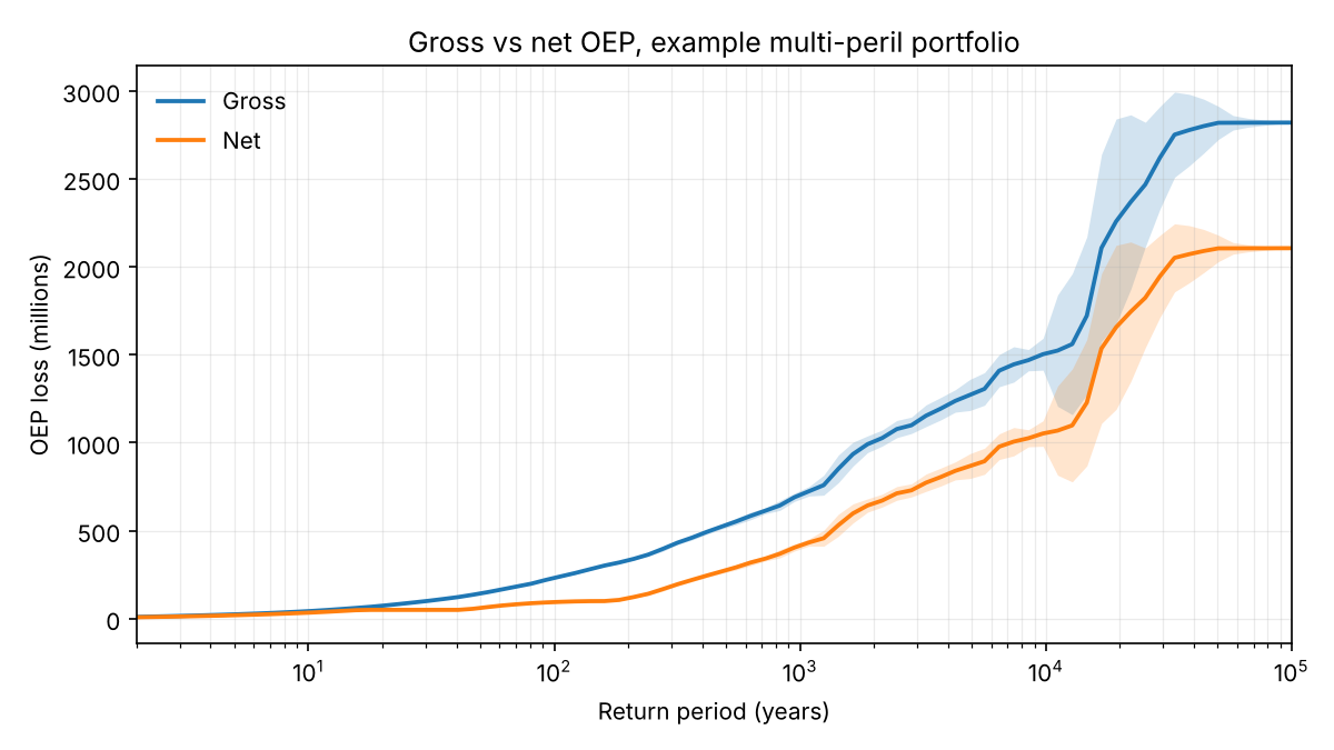
|
|
56
60
|
|
|
57
61
|
*Example portfolio: three perils, 20% quota share, a 50m xs 50m per-occurrence layer with two reinstatements, and a 100m aggregate stop-loss. The programme removes roughly two thirds of the 200-year occurrence loss — and the reinstatement cap is visible as the point where the net curve stops flattening.*
|
|
58
62
|
|
|
@@ -61,10 +65,12 @@ A reinsurer holds a portfolio exposed to several perils. The catastrophe models
|
|
|
61
65
|
## Install
|
|
62
66
|
|
|
63
67
|
```bash
|
|
64
|
-
pip install catagg
|
|
68
|
+
pip install --pre catagg # early pre-release on PyPI
|
|
69
|
+
# or the latest development version
|
|
70
|
+
pip install git+https://github.com/John-Amal/catagg
|
|
65
71
|
```
|
|
66
72
|
|
|
67
|
-
Python 3.11+. Runtime dependencies are numpy, pandas, pyarrow and scipy — nothing else.
|
|
73
|
+
Python 3.11+. Runtime dependencies are numpy, pandas, pyarrow and scipy — nothing else. `catagg` is in active development towards v0.1.0; the API below may still change.
|
|
68
74
|
|
|
69
75
|
---
|
|
70
76
|
|
|
@@ -73,34 +79,28 @@ Python 3.11+. Runtime dependencies are numpy, pandas, pyarrow and scipy — noth
|
|
|
73
79
|
```python
|
|
74
80
|
import catagg as ca
|
|
75
81
|
|
|
76
|
-
# 1.
|
|
77
|
-
elt = ca.
|
|
82
|
+
# 1. An event loss table (synthetic example portfolio; use ca.read_elt("portfolio.parquet") for your own)
|
|
83
|
+
elt = ca.swiss_multiperil_elt(n_events=1_000, seed=0)
|
|
78
84
|
|
|
79
85
|
# 2. Simulate 100,000 years
|
|
80
|
-
yelt = ca.simulate(
|
|
81
|
-
elt,
|
|
82
|
-
n_years=100_000,
|
|
83
|
-
frequency="negative_binomial", # or "poisson"
|
|
84
|
-
secondary_uncertainty=True,
|
|
85
|
-
seed=42,
|
|
86
|
-
)
|
|
86
|
+
yelt = ca.simulate(elt, n_years=100_000, secondary_uncertainty=True, seed=42)
|
|
87
87
|
|
|
88
88
|
# 3. Gross view
|
|
89
|
-
gross = ca.ep_curve(yelt)
|
|
89
|
+
gross = ca.ep_curve(yelt, kind="OEP")
|
|
90
90
|
print(gross.at_return_period([10, 50, 100, 200, 250]))
|
|
91
91
|
|
|
92
92
|
# 4. Apply a reinsurance programme
|
|
93
93
|
programme = ca.Programme([
|
|
94
94
|
ca.QuotaShare(cession=0.20),
|
|
95
|
-
ca.ExcessOfLoss(attachment=50e6, limit=50e6, reinstatements=2
|
|
95
|
+
ca.ExcessOfLoss(attachment=50e6, limit=50e6, reinstatements=2),
|
|
96
96
|
ca.AggregateStopLoss(attachment=100e6, limit=100e6),
|
|
97
97
|
])
|
|
98
|
-
|
|
99
98
|
result = programme.apply(yelt)
|
|
100
|
-
net = ca.ep_curve(result.
|
|
99
|
+
net = ca.ep_curve(result.yelt, kind="OEP", column="net_loss")
|
|
101
100
|
|
|
102
101
|
# 5. Compare
|
|
103
|
-
|
|
102
|
+
from catagg.plot import ep_comparison # pip install "catagg[plot]"
|
|
103
|
+
ep_comparison({"Gross": gross, "Net": net})
|
|
104
104
|
```
|
|
105
105
|
|
|
106
106
|
Everything runs from a clean clone — the example portfolio is generated synthetically by a documented generator, so there are no data dependencies and no licensing questions.
|
|
@@ -127,16 +127,15 @@ If you already work in cat modelling, skip this. If you're reading the code to l
|
|
|
127
127
|
|
|
128
128
|
**Frequency.** Poisson, or negative binomial where event clustering matters — European windstorm and hurricane seasons are both over-dispersed, and a Poisson assumption understates the aggregate tail.
|
|
129
129
|
|
|
130
|
-
**Secondary uncertainty.** Loss given occurrence is sampled from a beta distribution on `[0, exposed_value]`, fitted by moments to the ELT's mean and standard deviation,
|
|
130
|
+
**Secondary uncertainty.** Loss given occurrence is sampled from a beta distribution on `[0, exposed_value]`, fitted by moments to the ELT's mean and standard deviation. At the largest variance the support allows, that fit becomes the two-point law carrying probability mass at zero and at full exposure — the boundary member of the same family, reached continuously, rather than a free parameter. Degenerate cases — zero variance, or a variance the beta support cannot accommodate — are handled explicitly rather than silently clipped.
|
|
131
131
|
|
|
132
|
-
**Dependence.** Perils are
|
|
132
|
+
**Dependence.** Perils are currently simulated independently. Correlating them through a copula is on the roadmap.
|
|
133
133
|
|
|
134
134
|
**Financial structures.** Applied in programme order:
|
|
135
135
|
|
|
136
|
-
- Quota share
|
|
136
|
+
- Quota share
|
|
137
137
|
- Per-occurrence excess of loss: attachment, limit, *n* reinstatements at stated percentages, pro-rata to amount, with the aggregate cap of `limit × (1 + n)` enforced
|
|
138
138
|
- Aggregate excess of loss and stop-loss
|
|
139
|
-
- Franchise deductible
|
|
140
139
|
|
|
141
140
|
**Metrics.** OEP, AEP, AAL, TVaR at any return period, full return-period tables, and Monte Carlo standard errors on every tail statistic.
|
|
142
141
|
|
|
@@ -144,7 +143,7 @@ If you already work in cat modelling, skip this. If you're reading the code to l
|
|
|
144
143
|
|
|
145
144
|
## Validation
|
|
146
145
|
|
|
147
|
-
Numerical libraries in this domain live or die on whether you can show they're right. `catagg` ships a validation suite that runs in CI
|
|
146
|
+
Numerical libraries in this domain live or die on whether you can show they're right. `catagg` ships a validation suite that runs in CI on every commit:
|
|
148
147
|
|
|
149
148
|
- Simulated AAL converges to the analytic `Σ λᵢ · μᵢ`
|
|
150
149
|
- Sampled frequency moments match the specified Poisson or negative binomial
|
|
@@ -155,7 +154,7 @@ Numerical libraries in this domain live or die on whether you can show they're r
|
|
|
155
154
|
|
|
156
155
|
That last one matters more than it looks. A 200-year return period estimated from 10,000 simulation years carries a standard error large enough to change decisions, and most workflows never report it. `catagg` reports it by default.
|
|
157
156
|
|
|
158
|
-
See [docs/validation](https://john-amal.github.io/catagg/validation/).
|
|
157
|
+
See [docs/validation](https://john-amal.github.io/catagg/validation/); a readable validation notebook with published results is in progress.
|
|
159
158
|
|
|
160
159
|
---
|
|
161
160
|
|
|
@@ -171,6 +170,7 @@ See [docs/validation](https://john-amal.github.io/catagg/validation/).
|
|
|
171
170
|
|
|
172
171
|
## Roadmap
|
|
173
172
|
|
|
173
|
+
- **v0.1** — Gaussian and Student-t copulas across perils, ceding commission, franchise deductible, validation notebook
|
|
174
174
|
- **v0.2** — location and policy-level terms, surplus share, reinstatement premium calculation
|
|
175
175
|
- **v0.3** — OED-compatible ELT ingest, `oasislmf` interoperability
|
|
176
176
|
- **v0.4** — event-level correlation across sub-perils, seasonality in event timing
|
|
@@ -17,7 +17,7 @@ A reinsurer holds a portfolio exposed to several perils. The catastrophe models
|
|
|
17
17
|
|
|
18
18
|
`catagg` answers both. It simulates the year loss table, builds the gross exceedance probability curves, applies the reinsurance structures in the correct order, and returns gross, ceded and net views — with the validation checks that show the answer can be trusted.
|
|
19
19
|
|
|
20
|
-

|
|
20
|
+

|
|
21
21
|
|
|
22
22
|
*Example portfolio: three perils, 20% quota share, a 50m xs 50m per-occurrence layer with two reinstatements, and a 100m aggregate stop-loss. The programme removes roughly two thirds of the 200-year occurrence loss — and the reinstatement cap is visible as the point where the net curve stops flattening.*
|
|
23
23
|
|
|
@@ -26,10 +26,12 @@ A reinsurer holds a portfolio exposed to several perils. The catastrophe models
|
|
|
26
26
|
## Install
|
|
27
27
|
|
|
28
28
|
```bash
|
|
29
|
-
pip install catagg
|
|
29
|
+
pip install --pre catagg # early pre-release on PyPI
|
|
30
|
+
# or the latest development version
|
|
31
|
+
pip install git+https://github.com/John-Amal/catagg
|
|
30
32
|
```
|
|
31
33
|
|
|
32
|
-
Python 3.11+. Runtime dependencies are numpy, pandas, pyarrow and scipy — nothing else.
|
|
34
|
+
Python 3.11+. Runtime dependencies are numpy, pandas, pyarrow and scipy — nothing else. `catagg` is in active development towards v0.1.0; the API below may still change.
|
|
33
35
|
|
|
34
36
|
---
|
|
35
37
|
|
|
@@ -38,34 +40,28 @@ Python 3.11+. Runtime dependencies are numpy, pandas, pyarrow and scipy — noth
|
|
|
38
40
|
```python
|
|
39
41
|
import catagg as ca
|
|
40
42
|
|
|
41
|
-
# 1.
|
|
42
|
-
elt = ca.
|
|
43
|
+
# 1. An event loss table (synthetic example portfolio; use ca.read_elt("portfolio.parquet") for your own)
|
|
44
|
+
elt = ca.swiss_multiperil_elt(n_events=1_000, seed=0)
|
|
43
45
|
|
|
44
46
|
# 2. Simulate 100,000 years
|
|
45
|
-
yelt = ca.simulate(
|
|
46
|
-
elt,
|
|
47
|
-
n_years=100_000,
|
|
48
|
-
frequency="negative_binomial", # or "poisson"
|
|
49
|
-
secondary_uncertainty=True,
|
|
50
|
-
seed=42,
|
|
51
|
-
)
|
|
47
|
+
yelt = ca.simulate(elt, n_years=100_000, secondary_uncertainty=True, seed=42)
|
|
52
48
|
|
|
53
49
|
# 3. Gross view
|
|
54
|
-
gross = ca.ep_curve(yelt)
|
|
50
|
+
gross = ca.ep_curve(yelt, kind="OEP")
|
|
55
51
|
print(gross.at_return_period([10, 50, 100, 200, 250]))
|
|
56
52
|
|
|
57
53
|
# 4. Apply a reinsurance programme
|
|
58
54
|
programme = ca.Programme([
|
|
59
55
|
ca.QuotaShare(cession=0.20),
|
|
60
|
-
ca.ExcessOfLoss(attachment=50e6, limit=50e6, reinstatements=2
|
|
56
|
+
ca.ExcessOfLoss(attachment=50e6, limit=50e6, reinstatements=2),
|
|
61
57
|
ca.AggregateStopLoss(attachment=100e6, limit=100e6),
|
|
62
58
|
])
|
|
63
|
-
|
|
64
59
|
result = programme.apply(yelt)
|
|
65
|
-
net = ca.ep_curve(result.
|
|
60
|
+
net = ca.ep_curve(result.yelt, kind="OEP", column="net_loss")
|
|
66
61
|
|
|
67
62
|
# 5. Compare
|
|
68
|
-
|
|
63
|
+
from catagg.plot import ep_comparison # pip install "catagg[plot]"
|
|
64
|
+
ep_comparison({"Gross": gross, "Net": net})
|
|
69
65
|
```
|
|
70
66
|
|
|
71
67
|
Everything runs from a clean clone — the example portfolio is generated synthetically by a documented generator, so there are no data dependencies and no licensing questions.
|
|
@@ -92,16 +88,15 @@ If you already work in cat modelling, skip this. If you're reading the code to l
|
|
|
92
88
|
|
|
93
89
|
**Frequency.** Poisson, or negative binomial where event clustering matters — European windstorm and hurricane seasons are both over-dispersed, and a Poisson assumption understates the aggregate tail.
|
|
94
90
|
|
|
95
|
-
**Secondary uncertainty.** Loss given occurrence is sampled from a beta distribution on `[0, exposed_value]`, fitted by moments to the ELT's mean and standard deviation,
|
|
91
|
+
**Secondary uncertainty.** Loss given occurrence is sampled from a beta distribution on `[0, exposed_value]`, fitted by moments to the ELT's mean and standard deviation. At the largest variance the support allows, that fit becomes the two-point law carrying probability mass at zero and at full exposure — the boundary member of the same family, reached continuously, rather than a free parameter. Degenerate cases — zero variance, or a variance the beta support cannot accommodate — are handled explicitly rather than silently clipped.
|
|
96
92
|
|
|
97
|
-
**Dependence.** Perils are
|
|
93
|
+
**Dependence.** Perils are currently simulated independently. Correlating them through a copula is on the roadmap.
|
|
98
94
|
|
|
99
95
|
**Financial structures.** Applied in programme order:
|
|
100
96
|
|
|
101
|
-
- Quota share
|
|
97
|
+
- Quota share
|
|
102
98
|
- Per-occurrence excess of loss: attachment, limit, *n* reinstatements at stated percentages, pro-rata to amount, with the aggregate cap of `limit × (1 + n)` enforced
|
|
103
99
|
- Aggregate excess of loss and stop-loss
|
|
104
|
-
- Franchise deductible
|
|
105
100
|
|
|
106
101
|
**Metrics.** OEP, AEP, AAL, TVaR at any return period, full return-period tables, and Monte Carlo standard errors on every tail statistic.
|
|
107
102
|
|
|
@@ -109,7 +104,7 @@ If you already work in cat modelling, skip this. If you're reading the code to l
|
|
|
109
104
|
|
|
110
105
|
## Validation
|
|
111
106
|
|
|
112
|
-
Numerical libraries in this domain live or die on whether you can show they're right. `catagg` ships a validation suite that runs in CI
|
|
107
|
+
Numerical libraries in this domain live or die on whether you can show they're right. `catagg` ships a validation suite that runs in CI on every commit:
|
|
113
108
|
|
|
114
109
|
- Simulated AAL converges to the analytic `Σ λᵢ · μᵢ`
|
|
115
110
|
- Sampled frequency moments match the specified Poisson or negative binomial
|
|
@@ -120,7 +115,7 @@ Numerical libraries in this domain live or die on whether you can show they're r
|
|
|
120
115
|
|
|
121
116
|
That last one matters more than it looks. A 200-year return period estimated from 10,000 simulation years carries a standard error large enough to change decisions, and most workflows never report it. `catagg` reports it by default.
|
|
122
117
|
|
|
123
|
-
See [docs/validation](https://john-amal.github.io/catagg/validation/).
|
|
118
|
+
See [docs/validation](https://john-amal.github.io/catagg/validation/); a readable validation notebook with published results is in progress.
|
|
124
119
|
|
|
125
120
|
---
|
|
126
121
|
|
|
@@ -136,6 +131,7 @@ See [docs/validation](https://john-amal.github.io/catagg/validation/).
|
|
|
136
131
|
|
|
137
132
|
## Roadmap
|
|
138
133
|
|
|
134
|
+
- **v0.1** — Gaussian and Student-t copulas across perils, ceding commission, franchise deductible, validation notebook
|
|
139
135
|
- **v0.2** — location and policy-level terms, surplus share, reinstatement premium calculation
|
|
140
136
|
- **v0.3** — OED-compatible ELT ingest, `oasislmf` interoperability
|
|
141
137
|
- **v0.4** — event-level correlation across sub-perils, seasonality in event timing
|
|
@@ -0,0 +1,92 @@
|
|
|
1
|
+
# Financial structures
|
|
2
|
+
|
|
3
|
+
!!! note "v0.1.0 is in development"
|
|
4
|
+
|
|
5
|
+
This page documents loss-side reinsurance mechanics. Premium, ceding
|
|
6
|
+
commission and reinstatement premium are not yet modelled.
|
|
7
|
+
|
|
8
|
+
A `Programme` applies reinsurance structures to a simulated YELT and returns
|
|
9
|
+
gross, ceded and net loss on every occurrence.
|
|
10
|
+
|
|
11
|
+
```python
|
|
12
|
+
import catagg as ca
|
|
13
|
+
|
|
14
|
+
elt = ca.swiss_multiperil_elt(n_events=1_000, seed=0)
|
|
15
|
+
yelt = ca.simulate(elt, n_years=100_000, secondary_uncertainty=True, seed=42)
|
|
16
|
+
|
|
17
|
+
programme = ca.Programme([
|
|
18
|
+
ca.QuotaShare(cession=0.20),
|
|
19
|
+
ca.ExcessOfLoss(attachment=50e6, limit=50e6, reinstatements=2),
|
|
20
|
+
ca.AggregateStopLoss(attachment=100e6, limit=100e6),
|
|
21
|
+
])
|
|
22
|
+
result = programme.apply(yelt)
|
|
23
|
+
|
|
24
|
+
gross = ca.ep_curve(result.yelt, kind="OEP")
|
|
25
|
+
net = ca.ep_curve(result.yelt, kind="OEP", column="net_loss")
|
|
26
|
+
```
|
|
27
|
+
|
|
28
|
+
`result.yelt` holds `gross_loss`, `ceded_loss` and `net_loss` side by side, and
|
|
29
|
+
`result.ceded_by_structure` holds each structure's own cession, labelled by
|
|
30
|
+
position: `1_quota_share`, `2_excess_of_loss`, `3_aggregate_stop_loss`.
|
|
31
|
+
|
|
32
|
+
## Programme order is inuring order
|
|
33
|
+
|
|
34
|
+
Each structure protects what the structures before it left retained. In the
|
|
35
|
+
programme above the quota share takes 20% of every gross loss; the 50m xs 50m
|
|
36
|
+
layer then responds to the retained 80%, not to the gross; and the stop-loss
|
|
37
|
+
responds to what the layer left. Reversing two structures changes the answer,
|
|
38
|
+
so the order in the list is the order of application.
|
|
39
|
+
|
|
40
|
+
## Structures
|
|
41
|
+
|
|
42
|
+
| Structure | Pays, per occurrence | Running total |
|
|
43
|
+
|---|---|---|
|
|
44
|
+
| `QuotaShare(cession)` | `cession × retained` | None |
|
|
45
|
+
| `ExcessOfLoss(attachment, limit, reinstatements)` | Retained loss above `attachment`, up to `limit` | Annual cap `limit × (1 + reinstatements)`, or none if `reinstatements=None` |
|
|
46
|
+
| `AggregateStopLoss(attachment, limit)` | Its share of the annual recovery above `attachment` | Annual deductible, then annual `limit` |
|
|
47
|
+
|
|
48
|
+
`reinstatements` has no default. Market terms vary too much for any default to
|
|
49
|
+
be safe, and a silently assumed one would change every net figure.
|
|
50
|
+
|
|
51
|
+
`AggregateStopLoss` takes its attachment and limit in money, which also makes
|
|
52
|
+
it an aggregate excess of loss. A stop-loss quoted as a loss ratio converts to
|
|
53
|
+
this form given the subject premium.
|
|
54
|
+
|
|
55
|
+
## Order within the year
|
|
56
|
+
|
|
57
|
+
The per-occurrence layer's annual cap and the stop-loss's deductible and limit
|
|
58
|
+
are consumed in chronological order, using `occurrence_index` (see
|
|
59
|
+
[Simulation](simulation.md#occurrence-order-is-chronological)). A 50 xs 50
|
|
60
|
+
layer with two reinstatements pays at most 150 a year. Given layer losses of
|
|
61
|
+
30, 50, 50 and 40 in that order, the fourth recovers only the 20 left. In the
|
|
62
|
+
reverse order it is the 30 that is cut, to 10.
|
|
63
|
+
|
|
64
|
+
Order never changes a structure's annual total, so AAL and AEP of ceded and net
|
|
65
|
+
loss are unaffected by it. It does change which occurrence is cut off, and so
|
|
66
|
+
the net loss per occurrence and the **net OEP**. Allocating the stop-loss
|
|
67
|
+
recovery the same way is what gives a net OEP after an aggregate cover a
|
|
68
|
+
definite meaning.
|
|
69
|
+
|
|
70
|
+
## Conservation, in floating point
|
|
71
|
+
|
|
72
|
+
Net loss is what remains after each structure's cession is taken off in turn,
|
|
73
|
+
and `ceded_loss` is computed once, as `gross_loss − net_loss`. With that
|
|
74
|
+
construction `net_loss + ceded_loss` equals `gross_loss` to within one unit in
|
|
75
|
+
the last place on every occurrence: rounding one subtraction moves the result
|
|
76
|
+
by at most half a unit, and adding back at most doubles it.
|
|
77
|
+
|
|
78
|
+
That is the strongest form the identity can take in floating point. A bitwise
|
|
79
|
+
equality is not attainable: for a 20% quota share alone, a few percent of
|
|
80
|
+
occurrences differ from gross by one unit in the last place, whatever order the
|
|
81
|
+
arithmetic is done in.
|
|
82
|
+
|
|
83
|
+
`Programme.apply` also checks every structure's cession, including structures
|
|
84
|
+
written outside the library against the `Structure` protocol: none may be
|
|
85
|
+
negative, and none may exceed the loss it was offered. So net loss can never go
|
|
86
|
+
negative.
|
|
87
|
+
|
|
88
|
+
## API
|
|
89
|
+
|
|
90
|
+
::: catagg.financial.structures
|
|
91
|
+
|
|
92
|
+
::: catagg.financial.programme
|
|
Binary file
|
|
@@ -18,6 +18,7 @@ Python 3.11+. Runtime dependencies are numpy, pandas, pyarrow and scipy.
|
|
|
18
18
|
|
|
19
19
|
## Where to start
|
|
20
20
|
|
|
21
|
+
- **[Simulation](simulation.md)** — the ELT schema, frequency models and the year loop.
|
|
21
22
|
- **[Validation](validation.md)** — the checks that show the numbers can be trusted.
|
|
22
23
|
- **[API reference](api.md)** — the public surface.
|
|
23
24
|
- **[Changelog](changelog.md)** — what changed, and when.
|
|
@@ -0,0 +1,148 @@
|
|
|
1
|
+
# Metrics
|
|
2
|
+
|
|
3
|
+
!!! note "v0.1.0 is in development"
|
|
4
|
+
|
|
5
|
+
This page documents the gross view: EP curves, tail metrics and their Monte
|
|
6
|
+
Carlo error. For ceded and net curves, pass the result of a reinsurance
|
|
7
|
+
programme with `column="ceded_loss"` or `column="net_loss"`; see
|
|
8
|
+
[Financial structures](financial.md).
|
|
9
|
+
|
|
10
|
+
An exceedance probability curve is the empirical distribution of a per-year
|
|
11
|
+
loss, read from the tail. Two of them matter, and they answer different
|
|
12
|
+
questions.
|
|
13
|
+
|
|
14
|
+
**OEP**, occurrence exceedance probability, is the distribution of the largest
|
|
15
|
+
single event in a year. It is what a per-occurrence layer responds to.
|
|
16
|
+
**AEP**, aggregate exceedance probability, is the distribution of total annual
|
|
17
|
+
loss. It is what aggregate cover and capital respond to. Both come from the
|
|
18
|
+
same year loss table, so one simulation gives you both.
|
|
19
|
+
|
|
20
|
+
```python
|
|
21
|
+
import catagg as ca
|
|
22
|
+
|
|
23
|
+
elt = ca.swiss_multiperil_elt(n_events=400, seed=0)
|
|
24
|
+
yelt = ca.simulate(elt, n_years=50_000, seed=1, secondary_uncertainty=True)
|
|
25
|
+
|
|
26
|
+
aggregate = ca.ep_curve(yelt, kind="AEP")
|
|
27
|
+
print(aggregate.at_return_period([100, 200, 250]))
|
|
28
|
+
print(aggregate.tvar(200))
|
|
29
|
+
```
|
|
30
|
+
|
|
31
|
+
`EPCurve` keeps the whole per-year loss vector rather than a summarised curve,
|
|
32
|
+
so any return period, tail metric or standard error can be read afterwards
|
|
33
|
+
without re-simulating.
|
|
34
|
+
|
|
35
|
+
## Return periods, and which plotting position
|
|
36
|
+
|
|
37
|
+
A return period $R$ is the reciprocal of an annual exceedance probability, so
|
|
38
|
+
the loss at $R$ is the $1 - 1/R$ quantile of the annual loss. The quantile uses
|
|
39
|
+
the **Weibull plotting position**, $k / (n + 1)$ for the $k$-th largest of $n$
|
|
40
|
+
simulated years.
|
|
41
|
+
|
|
42
|
+
That is not a cosmetic choice. For a continuous distribution $k / (n + 1)$ is
|
|
43
|
+
unbiased for the exceedance probability of the $k$-th order statistic. The
|
|
44
|
+
$k / n$ convention some vendor tools use is biased, and it cannot represent the
|
|
45
|
+
largest simulated year at all without assigning it a zero exceedance
|
|
46
|
+
probability — an infinite return period from one observation.
|
|
47
|
+
|
|
48
|
+
## Refusing to extrapolate
|
|
49
|
+
|
|
50
|
+
`at_return_period` raises rather than answering when the return period is longer
|
|
51
|
+
than the simulation:
|
|
52
|
+
|
|
53
|
+
```pycon
|
|
54
|
+
>>> curve = ca.ep_curve(ca.simulate(elt, n_years=10_000, seed=1), kind="AEP")
|
|
55
|
+
>>> curve.at_return_period(10_000)
|
|
56
|
+
CataggError: return_period 10000 exceeds the 10000 simulated years...
|
|
57
|
+
```
|
|
58
|
+
|
|
59
|
+
Reading a 1-in-10,000 loss off 10,000 simulated years returns the single largest
|
|
60
|
+
year and dresses one observation up as a return period. The library will not do
|
|
61
|
+
it quietly.
|
|
62
|
+
|
|
63
|
+
## TVaR
|
|
64
|
+
|
|
65
|
+
Tail value at risk is the mean loss in the years that exceed a return period, so
|
|
66
|
+
it answers what capital regimes actually ask: not "how bad is the 1-in-200 year"
|
|
67
|
+
but "how bad is the average year worse than that". It is computed as the
|
|
68
|
+
integrated expected shortfall over the largest $n / R$ years, with a fractional
|
|
69
|
+
weight on the boundary year so the figure stays continuous in $R$ rather than
|
|
70
|
+
jumping as the count crosses an integer.
|
|
71
|
+
|
|
72
|
+
## Standard error is not optional
|
|
73
|
+
|
|
74
|
+
Every figure this module returns carries the Monte Carlo standard error of the
|
|
75
|
+
estimate, because a return period read off a simulation is a statistic and
|
|
76
|
+
carries sampling error like any other. For the example portfolio the RP-200 AEP
|
|
77
|
+
estimated from 10,000 simulation years has a standard error of around 8% —
|
|
78
|
+
large enough to move a reinsurance decision, and almost never reported.
|
|
79
|
+
|
|
80
|
+
Neither estimator introduces a tuning constant, and both are checked against a
|
|
81
|
+
replication study rather than asserted.
|
|
82
|
+
|
|
83
|
+
### Quantiles
|
|
84
|
+
|
|
85
|
+
The empirical CDF at the quantile has standard deviation
|
|
86
|
+
$\sqrt{p(1-p)/n}$. Perturbing the probability level by exactly that amount and
|
|
87
|
+
reading the quantile function at both ends gives the sampling spread of the
|
|
88
|
+
estimate, mapped through the distribution's own shape:
|
|
89
|
+
|
|
90
|
+
$$\text{se} = \frac{Q(u + h) - Q(u - h)}{2}, \qquad u = 1 - p, \quad h = \sqrt{\frac{p\,(1-p)}{n}}$$
|
|
91
|
+
|
|
92
|
+
This is the Siddiqui density-quantile estimator with the bandwidth pinned to the
|
|
93
|
+
statistically natural scale rather than chosen. It needs no density estimate and
|
|
94
|
+
degrades correctly in the far tail, where the spacing between order statistics
|
|
95
|
+
is wide.
|
|
96
|
+
|
|
97
|
+
### TVaR, and the mistake worth naming
|
|
98
|
+
|
|
99
|
+
The tail mean over $k = np$ years is a mean, so the obvious estimator of its
|
|
100
|
+
error is $s_{\text{tail}} / \sqrt{k}$.
|
|
101
|
+
|
|
102
|
+
That estimator is wrong, and wrong in the dangerous direction. It treats the
|
|
103
|
+
exceedance threshold as known when the threshold is itself estimated from the
|
|
104
|
+
same sample. Against a replication study it **understates the true error by
|
|
105
|
+
between a fifth and a third**. The correction restores what it omits:
|
|
106
|
+
|
|
107
|
+
$$\text{se} = \sqrt{\frac{s_{\text{tail}}^2 + (1 - p)\,(\text{TVaR} - \text{VaR})^2}{k}}$$
|
|
108
|
+
|
|
109
|
+
### How well they do
|
|
110
|
+
|
|
111
|
+
Measured against 30 independent reruns of the same portfolio, as the ratio of
|
|
112
|
+
the error a single run reports to the spread actually observed across runs:
|
|
113
|
+
|
|
114
|
+
| Simulated years | Quantile | TVaR |
|
|
115
|
+
|---|---|---|
|
|
116
|
+
| 10,000 | 1.14 | 1.15 |
|
|
117
|
+
| 100,000 | 0.98 | 0.99 |
|
|
118
|
+
|
|
119
|
+
Both run slightly conservative at short simulations, which is the right
|
|
120
|
+
direction for a number whose purpose is to stop someone over-reading a tail.
|
|
121
|
+
The tests assert this ratio directly, so a change that quietly breaks an error
|
|
122
|
+
estimate fails rather than shipping a comfortable, wrong number.
|
|
123
|
+
|
|
124
|
+
## Plotting
|
|
125
|
+
|
|
126
|
+
matplotlib is **not** a runtime dependency. The engine needs numpy, pandas,
|
|
127
|
+
pyarrow and scipy, and a library that forces a plotting stack on everyone who
|
|
128
|
+
imports it has made a decision on their behalf. Install the extra:
|
|
129
|
+
|
|
130
|
+
```bash
|
|
131
|
+
pip install catagg[plot]
|
|
132
|
+
```
|
|
133
|
+
|
|
134
|
+
```python
|
|
135
|
+
from catagg.plot import ep_comparison
|
|
136
|
+
|
|
137
|
+
ep_comparison({"Gross": aggregate}, title="Swiss multi-peril, gross")
|
|
138
|
+
```
|
|
139
|
+
|
|
140
|
+
The shaded band is plus or minus one standard error, drawn by default. At the
|
|
141
|
+
long return periods on the right of the plot it is wide enough to change a
|
|
142
|
+
decision, and a curve drawn as a clean line hides that.
|
|
143
|
+
|
|
144
|
+
## API
|
|
145
|
+
|
|
146
|
+
::: catagg.metrics.ep
|
|
147
|
+
|
|
148
|
+
::: catagg.plot
|