adopt-plot 0.1.9__tar.gz → 0.2.9__tar.gz
This diff represents the content of publicly available package versions that have been released to one of the supported registries. The information contained in this diff is provided for informational purposes only and reflects changes between package versions as they appear in their respective public registries.
- {adopt_plot-0.1.9 → adopt_plot-0.2.9}/LICENSE +21 -21
- {adopt_plot-0.1.9/src/adopt_plot.egg-info → adopt_plot-0.2.9}/PKG-INFO +98 -98
- {adopt_plot-0.1.9 → adopt_plot-0.2.9}/README.md +82 -82
- {adopt_plot-0.1.9 → adopt_plot-0.2.9}/pyproject.toml +27 -27
- {adopt_plot-0.1.9 → adopt_plot-0.2.9}/setup.cfg +4 -4
- {adopt_plot-0.1.9 → adopt_plot-0.2.9}/src/adopt_plot/__init__.py +10 -10
- {adopt_plot-0.1.9 → adopt_plot-0.2.9}/src/adopt_plot/plot.py +446 -427
- {adopt_plot-0.1.9 → adopt_plot-0.2.9/src/adopt_plot.egg-info}/PKG-INFO +98 -98
- {adopt_plot-0.1.9 → adopt_plot-0.2.9}/src/adopt_plot.egg-info/SOURCES.txt +0 -0
- {adopt_plot-0.1.9 → adopt_plot-0.2.9}/src/adopt_plot.egg-info/dependency_links.txt +0 -0
- {adopt_plot-0.1.9 → adopt_plot-0.2.9}/src/adopt_plot.egg-info/requires.txt +0 -0
- {adopt_plot-0.1.9 → adopt_plot-0.2.9}/src/adopt_plot.egg-info/top_level.txt +0 -0
|
@@ -1,22 +1,22 @@
|
|
|
1
|
-
Copyright (c) 2026 VartRusData.
|
|
2
|
-
|
|
3
|
-
Redistribution and use in source and binary forms, with or without modification,
|
|
4
|
-
are permitted provided that the following conditions are met:
|
|
5
|
-
|
|
6
|
-
1. Redistributions of source code must retain the above copyright notice,
|
|
7
|
-
this list of conditions and the following disclaimer.
|
|
8
|
-
2. Redistributions in binary form must reproduce the above copyright notice,
|
|
9
|
-
this list of conditions and the following disclaimer in the documentation and/or other materials provided
|
|
10
|
-
with the distribution.
|
|
11
|
-
3. Neither the name of the copyright holder nor the names of its contributors
|
|
12
|
-
may be used to endorse or promote products derived from this software
|
|
13
|
-
without specific prior written permission.
|
|
14
|
-
THIS SOFTWARE IS PROVIDED BY THE COPYRIGHT HOLDERS AND CONTRIBUTORS "AS IS"
|
|
15
|
-
AND ANY EXPRESS OR IMPLIED WARRANTIES, INCLUDING, BUT NOT LIMITED TO,
|
|
16
|
-
THE IMPLIED WARRANTIES OF MERCHANTABILITY AND FITNESS FOR A PARTICULAR PURPOSE ARE DISCLAIMED.
|
|
17
|
-
IN NO EVENT SHALL THE COPYRIGHT HOLDER OR CONTRIBUTORS BE LIABLE FOR ANY DIRECT,
|
|
18
|
-
INDIRECT, INCIDENTAL, SPECIAL, EXEMPLARY, OR CONSEQUENTIAL DAMAGES
|
|
19
|
-
(INCLUDING, BUT NOT LIMITED TO, PROCUREMENT OF SUBSTITUTE GOODS OR SERVICES; LOSS OF USE, DATA,
|
|
20
|
-
OR PROFITS; OR BUSINESS INTERRUPTION) HOWEVER CAUSED AND ON ANY THEORY OF LIABILITY, WHETHER IN CONTRACT,
|
|
21
|
-
STRICT LIABILITY, OR TORT (INCLUDING NEGLIGENCE OR OTHERWISE) ARISING IN ANY WAY OUT OF THE USE
|
|
1
|
+
Copyright (c) 2026 VartRusData.
|
|
2
|
+
|
|
3
|
+
Redistribution and use in source and binary forms, with or without modification,
|
|
4
|
+
are permitted provided that the following conditions are met:
|
|
5
|
+
|
|
6
|
+
1. Redistributions of source code must retain the above copyright notice,
|
|
7
|
+
this list of conditions and the following disclaimer.
|
|
8
|
+
2. Redistributions in binary form must reproduce the above copyright notice,
|
|
9
|
+
this list of conditions and the following disclaimer in the documentation and/or other materials provided
|
|
10
|
+
with the distribution.
|
|
11
|
+
3. Neither the name of the copyright holder nor the names of its contributors
|
|
12
|
+
may be used to endorse or promote products derived from this software
|
|
13
|
+
without specific prior written permission.
|
|
14
|
+
THIS SOFTWARE IS PROVIDED BY THE COPYRIGHT HOLDERS AND CONTRIBUTORS "AS IS"
|
|
15
|
+
AND ANY EXPRESS OR IMPLIED WARRANTIES, INCLUDING, BUT NOT LIMITED TO,
|
|
16
|
+
THE IMPLIED WARRANTIES OF MERCHANTABILITY AND FITNESS FOR A PARTICULAR PURPOSE ARE DISCLAIMED.
|
|
17
|
+
IN NO EVENT SHALL THE COPYRIGHT HOLDER OR CONTRIBUTORS BE LIABLE FOR ANY DIRECT,
|
|
18
|
+
INDIRECT, INCIDENTAL, SPECIAL, EXEMPLARY, OR CONSEQUENTIAL DAMAGES
|
|
19
|
+
(INCLUDING, BUT NOT LIMITED TO, PROCUREMENT OF SUBSTITUTE GOODS OR SERVICES; LOSS OF USE, DATA,
|
|
20
|
+
OR PROFITS; OR BUSINESS INTERRUPTION) HOWEVER CAUSED AND ON ANY THEORY OF LIABILITY, WHETHER IN CONTRACT,
|
|
21
|
+
STRICT LIABILITY, OR TORT (INCLUDING NEGLIGENCE OR OTHERWISE) ARISING IN ANY WAY OUT OF THE USE
|
|
22
22
|
OF THIS SOFTWARE, EVEN IF ADVISED OF THE POSSIBILITY OF SUCH DAMAGE.
|
|
@@ -1,98 +1,98 @@
|
|
|
1
|
-
Metadata-Version: 2.4
|
|
2
|
-
Name: adopt-plot
|
|
3
|
-
Version: 0.
|
|
4
|
-
Summary: A universal plotter for implicit functions using adaptive engine selection.
|
|
5
|
-
Author: VartRusData
|
|
6
|
-
License: BSD 3-Clause
|
|
7
|
-
Classifier: License :: OSI Approved :: BSD License
|
|
8
|
-
Requires-Python: >=3.9
|
|
9
|
-
Description-Content-Type: text/markdown
|
|
10
|
-
License-File: LICENSE
|
|
11
|
-
Requires-Dist: sympy
|
|
12
|
-
Requires-Dist: matplotlib
|
|
13
|
-
Requires-Dist: numpy
|
|
14
|
-
Dynamic: license-file
|
|
15
|
-
|
|
16
|
-
# adopt-plot
|
|
17
|
-
### Or AdoptPlot
|
|
18
|
-
A library for plotting implicit functions using two rendering engines:
|
|
19
|
-
|
|
20
|
-
- `contour` from `matplotlib`.
|
|
21
|
-
- `plot_implicit` from `sympy` which internally uses **Adaptive Marching Squares (AMR)** — an adaptive algorithm that correctly handles the domain of definition and discontinuities.
|
|
22
|
-
|
|
23
|
-
**Automatic selection:** If the equation has domain restrictions (e.g., logarithm or square root), `plot_implicit` is used. If the function is smooth, the fast `contour` engine is chosen. Visually, they are indistinguishable, but the best algorithm is selected automatically.
|
|
24
|
-
|
|
25
|
-
---
|
|
26
|
-
|
|
27
|
-
## Installation
|
|
28
|
-
|
|
29
|
-
```bash
|
|
30
|
-
pip install adopt-plot
|
|
31
|
-
```
|
|
32
|
-
## Quick Start
|
|
33
|
-
Plot a graph in one line:
|
|
34
|
-
|
|
35
|
-
```python
|
|
36
|
-
from adopt_plot import AdoptPlot
|
|
37
|
-
|
|
38
|
-
# The plot will open immediately
|
|
39
|
-
plot = AdoptPlot("y = 2*x + 2")
|
|
40
|
-
```
|
|
41
|
-
Or with deferred display (to add custom elements first):
|
|
42
|
-
|
|
43
|
-
```python
|
|
44
|
-
from adopt_plot import AdoptPlot
|
|
45
|
-
|
|
46
|
-
plot = AdoptPlot("y = sqrt(x)", show=False)
|
|
47
|
-
# Add custom elements here:
|
|
48
|
-
plot.ax.scatter(2, 2, color='red')
|
|
49
|
-
plot.show()
|
|
50
|
-
# Show the plot after modifications
|
|
51
|
-
```
|
|
52
|
-
All plot elements (`axes`, `fig`, `plt`) are accessible via the plot object and its attributes:
|
|
53
|
-
|
|
54
|
-
```python
|
|
55
|
-
from adopt_plot import AdoptPlot
|
|
56
|
-
plot = AdoptPlot("y = 1/x", show=False)
|
|
57
|
-
plot.ax.set_xlim(-10, 10) # Change X-axis limits
|
|
58
|
-
plot.save("my_plot.png", dpi=300)# Save to file
|
|
59
|
-
```
|
|
60
|
-
[]($y=1/x$)
|
|
61
|
-
```python
|
|
62
|
-
from adopt_plot import AdoptPlot
|
|
63
|
-
|
|
64
|
-
plot = AdoptPlot("sin(sqrt(x**2 + y**2)) / log(x**2 + y**2 + 1) = 0", show=False)
|
|
65
|
-
|
|
66
|
-
# Подкручиваем стиль под публикацию
|
|
67
|
-
plot.ax.set_title("Implicit function with radial oscillations")
|
|
68
|
-
plot.ax.grid(True, linestyle=':', alpha=0.5)
|
|
69
|
-
|
|
70
|
-
# Сохраняем с высоким DPI
|
|
71
|
-
plot.save("publication_ready.png", dpi=300, bbox_inches='tight')
|
|
72
|
-
plot.show()
|
|
73
|
-
```
|
|
74
|
-
[]($sin(sqrt(x^2+y^2))/log(x^2+y^2+1)=0$)
|
|
75
|
-
## Methods
|
|
76
|
-
- **`show`**: Show the figure
|
|
77
|
-
- **`save`**: Save the figure
|
|
78
|
-
## Parameters
|
|
79
|
-
|
|
80
|
-
When creating an `AdoptPlot` object, the following parameters are available:
|
|
81
|
-
|
|
82
|
-
- **`expr`** (`str`): The equation string (e.g., `"y = 1/x"`).
|
|
83
|
-
- **`lib`** (`Literal['contour', 'implicit', None]`): Forced rendering engine. Default is `None` (automatic selection).
|
|
84
|
-
- **`xlims`, `ylims`** (`Tuple[float, float]`): Initial visible range for the plot. Default `(-20, 20)`.
|
|
85
|
-
- **`n`** (`int`): Grid density for the `contour` engine. Default `
|
|
86
|
-
- **`depth`** (`int`): Adaptive refinement depth for `plot_implicit`. Default `9`.
|
|
87
|
-
- **`linewidth`** (`float`): Thickness of the plot line. Default `2.0`.
|
|
88
|
-
- **`limit`** (`float | Tuple[float, float, float, float]`): Computational domain. Pass a single number (square) or a tuple of 4 numbers `(x_min, x_max, y_min, y_max)`. Default `100`.
|
|
89
|
-
- **`color`** (`str`): Line color. Default `'blue'`.
|
|
90
|
-
- **`legend`** (`bool`): Whether to display the legend. Default `True`.
|
|
91
|
-
- **`points`** (`bool`): Whether to display axis intersection points. Default `True`.
|
|
92
|
-
- **`grid`** (`bool`): Whether to display the grid. Default `True`.
|
|
93
|
-
- **`interact`** (`bool`): Allow zooming and panning via keyboard (`Ctrl +` and `Ctrl -`). Default `True`.
|
|
94
|
-
- **`show`** (`bool`): If `False`, the plot does not open immediately, allowing you to add elements. Default `True`.
|
|
95
|
-
- **`text_legend`** (`str`): Additional text for the legend. Default `None`.
|
|
96
|
-
## License
|
|
97
|
-
|
|
98
|
-
Distributed under the **BSD 3-Clause** license.
|
|
1
|
+
Metadata-Version: 2.4
|
|
2
|
+
Name: adopt-plot
|
|
3
|
+
Version: 0.2.9
|
|
4
|
+
Summary: A universal plotter for implicit functions using adaptive engine selection.
|
|
5
|
+
Author: VartRusData
|
|
6
|
+
License: BSD 3-Clause
|
|
7
|
+
Classifier: License :: OSI Approved :: BSD License
|
|
8
|
+
Requires-Python: >=3.9
|
|
9
|
+
Description-Content-Type: text/markdown
|
|
10
|
+
License-File: LICENSE
|
|
11
|
+
Requires-Dist: sympy
|
|
12
|
+
Requires-Dist: matplotlib
|
|
13
|
+
Requires-Dist: numpy
|
|
14
|
+
Dynamic: license-file
|
|
15
|
+
|
|
16
|
+
# adopt-plot
|
|
17
|
+
### Or AdoptPlot
|
|
18
|
+
A library for plotting implicit functions using two rendering engines:
|
|
19
|
+
|
|
20
|
+
- `contour` from `matplotlib`.
|
|
21
|
+
- `plot_implicit` from `sympy` which internally uses **Adaptive Marching Squares (AMR)** — an adaptive algorithm that correctly handles the domain of definition and discontinuities.
|
|
22
|
+
|
|
23
|
+
**Automatic selection:** If the equation has domain restrictions (e.g., logarithm or square root), `plot_implicit` is used. If the function is smooth, the fast `contour` engine is chosen. Visually, they are indistinguishable, but the best algorithm is selected automatically.
|
|
24
|
+
|
|
25
|
+
---
|
|
26
|
+
|
|
27
|
+
## Installation
|
|
28
|
+
|
|
29
|
+
```bash
|
|
30
|
+
pip install adopt-plot
|
|
31
|
+
```
|
|
32
|
+
## Quick Start
|
|
33
|
+
Plot a graph in one line:
|
|
34
|
+
|
|
35
|
+
```python
|
|
36
|
+
from adopt_plot import AdoptPlot
|
|
37
|
+
|
|
38
|
+
# The plot will open immediately
|
|
39
|
+
plot = AdoptPlot("y = 2*x + 2")
|
|
40
|
+
```
|
|
41
|
+
Or with deferred display (to add custom elements first):
|
|
42
|
+
|
|
43
|
+
```python
|
|
44
|
+
from adopt_plot import AdoptPlot
|
|
45
|
+
|
|
46
|
+
plot = AdoptPlot("y = sqrt(x)", show=False)
|
|
47
|
+
# Add custom elements here:
|
|
48
|
+
plot.ax.scatter(2, 2, color='red')
|
|
49
|
+
plot.show()
|
|
50
|
+
# Show the plot after modifications
|
|
51
|
+
```
|
|
52
|
+
All plot elements (`axes`, `fig`, `plt`) are accessible via the plot object and its attributes:
|
|
53
|
+
|
|
54
|
+
```python
|
|
55
|
+
from adopt_plot import AdoptPlot
|
|
56
|
+
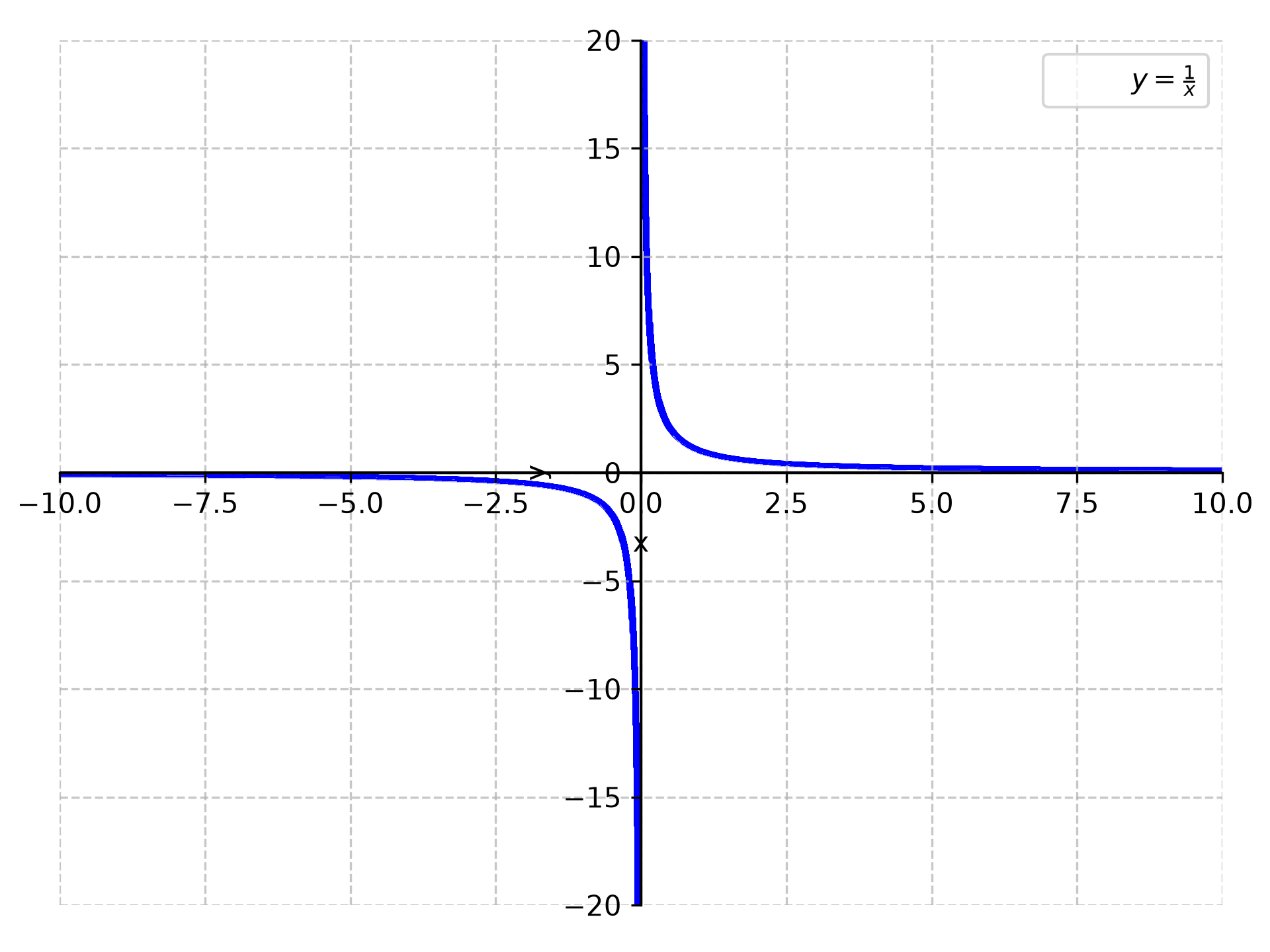
plot = AdoptPlot("y = 1/x", show=False)
|
|
57
|
+
plot.ax.set_xlim(-10, 10) # Change X-axis limits
|
|
58
|
+
plot.save("my_plot.png", dpi=300)# Save to file
|
|
59
|
+
```
|
|
60
|
+
[]($y=1/x$)
|
|
61
|
+
```python
|
|
62
|
+
from adopt_plot import AdoptPlot
|
|
63
|
+
|
|
64
|
+
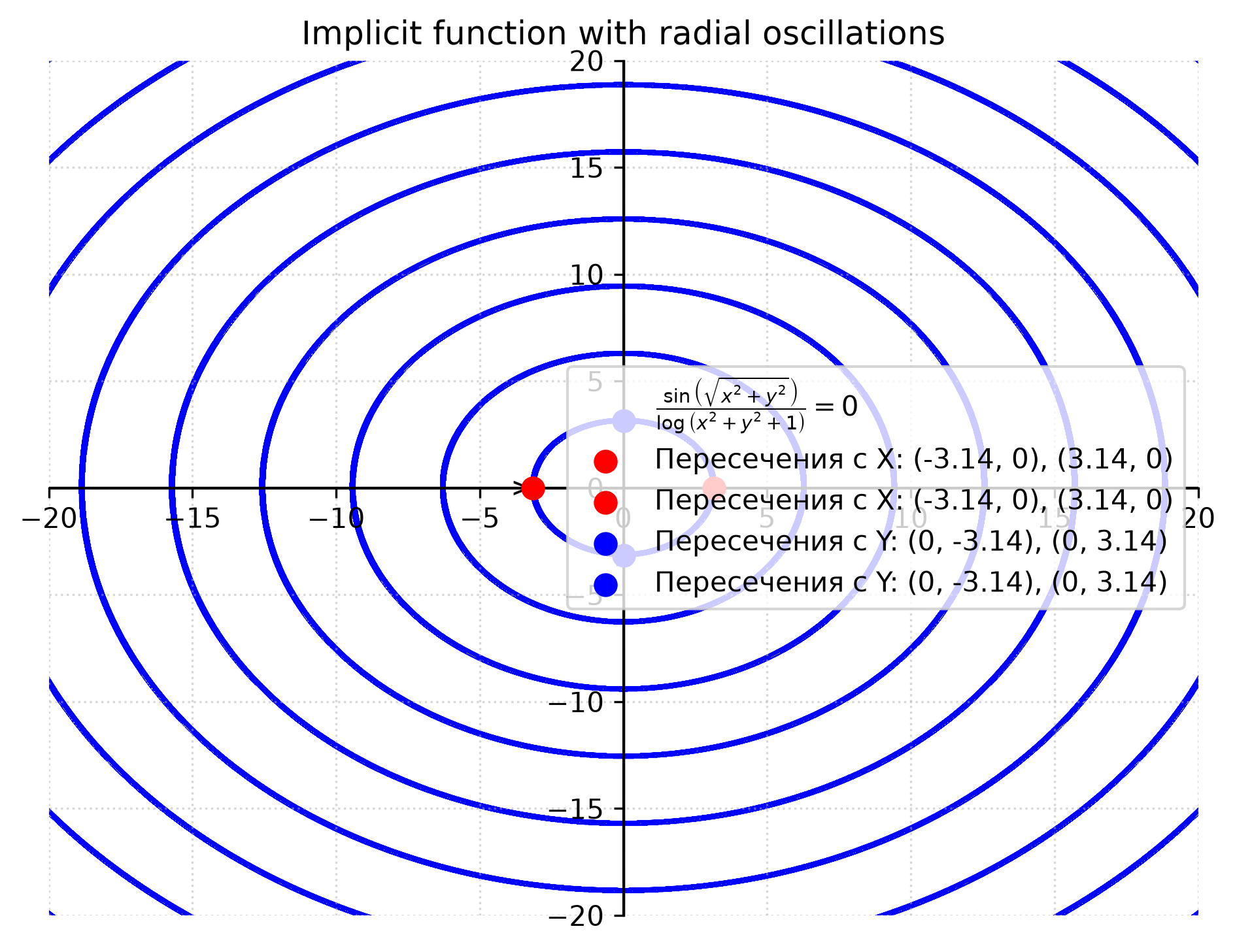
plot = AdoptPlot("sin(sqrt(x**2 + y**2)) / log(x**2 + y**2 + 1) = 0", show=False)
|
|
65
|
+
|
|
66
|
+
# Подкручиваем стиль под публикацию
|
|
67
|
+
plot.ax.set_title("Implicit function with radial oscillations")
|
|
68
|
+
plot.ax.grid(True, linestyle=':', alpha=0.5)
|
|
69
|
+
|
|
70
|
+
# Сохраняем с высоким DPI
|
|
71
|
+
plot.save("publication_ready.png", dpi=300, bbox_inches='tight')
|
|
72
|
+
plot.show()
|
|
73
|
+
```
|
|
74
|
+
[]($sin(sqrt(x^2+y^2))/log(x^2+y^2+1)=0$)
|
|
75
|
+
## Methods
|
|
76
|
+
- **`show`**: Show the figure
|
|
77
|
+
- **`save`**: Save the figure
|
|
78
|
+
## Parameters
|
|
79
|
+
|
|
80
|
+
When creating an `AdoptPlot` object, the following parameters are available:
|
|
81
|
+
|
|
82
|
+
- **`expr`** (`str`): The equation string (e.g., `"y = 1/x"`).
|
|
83
|
+
- **`lib`** (`Literal['contour', 'implicit', None]`): Forced rendering engine. Default is `None` (automatic selection).
|
|
84
|
+
- **`xlims`, `ylims`** (`Tuple[float, float]`): Initial visible range for the plot. Default `(-20, 20)`.
|
|
85
|
+
- **`n`** (`int`): Grid density for the `contour` engine. Default `1300`.
|
|
86
|
+
- **`depth`** (`int`): Adaptive refinement depth for `plot_implicit`. Default `9`.
|
|
87
|
+
- **`linewidth`** (`float`): Thickness of the plot line. Default `2.0`.
|
|
88
|
+
- **`limit`** (`float | Tuple[float, float, float, float]`): Computational domain. Pass a single number (square) or a tuple of 4 numbers `(x_min, x_max, y_min, y_max)`. Default `100`.
|
|
89
|
+
- **`color`** (`str`): Line color. Default `'blue'`.
|
|
90
|
+
- **`legend`** (`bool`): Whether to display the legend. Default `True`.
|
|
91
|
+
- **`points`** (`bool`): Whether to display axis intersection points. Default `True`.
|
|
92
|
+
- **`grid`** (`bool`): Whether to display the grid. Default `True`.
|
|
93
|
+
- **`interact`** (`bool`): Allow zooming and panning via keyboard (`Ctrl +` and `Ctrl -`). Default `True`.
|
|
94
|
+
- **`show`** (`bool`): If `False`, the plot does not open immediately, allowing you to add elements. Default `True`.
|
|
95
|
+
- **`text_legend`** (`str`): Additional text for the legend. Default `None`.
|
|
96
|
+
## License
|
|
97
|
+
|
|
98
|
+
Distributed under the **BSD 3-Clause** license.
|
|
@@ -1,83 +1,83 @@
|
|
|
1
|
-
# adopt-plot
|
|
2
|
-
### Or AdoptPlot
|
|
3
|
-
A library for plotting implicit functions using two rendering engines:
|
|
4
|
-
|
|
5
|
-
- `contour` from `matplotlib`.
|
|
6
|
-
- `plot_implicit` from `sympy` which internally uses **Adaptive Marching Squares (AMR)** — an adaptive algorithm that correctly handles the domain of definition and discontinuities.
|
|
7
|
-
|
|
8
|
-
**Automatic selection:** If the equation has domain restrictions (e.g., logarithm or square root), `plot_implicit` is used. If the function is smooth, the fast `contour` engine is chosen. Visually, they are indistinguishable, but the best algorithm is selected automatically.
|
|
9
|
-
|
|
10
|
-
---
|
|
11
|
-
|
|
12
|
-
## Installation
|
|
13
|
-
|
|
14
|
-
```bash
|
|
15
|
-
pip install adopt-plot
|
|
16
|
-
```
|
|
17
|
-
## Quick Start
|
|
18
|
-
Plot a graph in one line:
|
|
19
|
-
|
|
20
|
-
```python
|
|
21
|
-
from adopt_plot import AdoptPlot
|
|
22
|
-
|
|
23
|
-
# The plot will open immediately
|
|
24
|
-
plot = AdoptPlot("y = 2*x + 2")
|
|
25
|
-
```
|
|
26
|
-
Or with deferred display (to add custom elements first):
|
|
27
|
-
|
|
28
|
-
```python
|
|
29
|
-
from adopt_plot import AdoptPlot
|
|
30
|
-
|
|
31
|
-
plot = AdoptPlot("y = sqrt(x)", show=False)
|
|
32
|
-
# Add custom elements here:
|
|
33
|
-
plot.ax.scatter(2, 2, color='red')
|
|
34
|
-
plot.show()
|
|
35
|
-
# Show the plot after modifications
|
|
36
|
-
```
|
|
37
|
-
All plot elements (`axes`, `fig`, `plt`) are accessible via the plot object and its attributes:
|
|
38
|
-
|
|
39
|
-
```python
|
|
40
|
-
from adopt_plot import AdoptPlot
|
|
41
|
-
plot = AdoptPlot("y = 1/x", show=False)
|
|
42
|
-
plot.ax.set_xlim(-10, 10) # Change X-axis limits
|
|
43
|
-
plot.save("my_plot.png", dpi=300)# Save to file
|
|
44
|
-
```
|
|
45
|
-
[]($y=1/x$)
|
|
46
|
-
```python
|
|
47
|
-
from adopt_plot import AdoptPlot
|
|
48
|
-
|
|
49
|
-
plot = AdoptPlot("sin(sqrt(x**2 + y**2)) / log(x**2 + y**2 + 1) = 0", show=False)
|
|
50
|
-
|
|
51
|
-
# Подкручиваем стиль под публикацию
|
|
52
|
-
plot.ax.set_title("Implicit function with radial oscillations")
|
|
53
|
-
plot.ax.grid(True, linestyle=':', alpha=0.5)
|
|
54
|
-
|
|
55
|
-
# Сохраняем с высоким DPI
|
|
56
|
-
plot.save("publication_ready.png", dpi=300, bbox_inches='tight')
|
|
57
|
-
plot.show()
|
|
58
|
-
```
|
|
59
|
-
[]($sin(sqrt(x^2+y^2))/log(x^2+y^2+1)=0$)
|
|
60
|
-
## Methods
|
|
61
|
-
- **`show`**: Show the figure
|
|
62
|
-
- **`save`**: Save the figure
|
|
63
|
-
## Parameters
|
|
64
|
-
|
|
65
|
-
When creating an `AdoptPlot` object, the following parameters are available:
|
|
66
|
-
|
|
67
|
-
- **`expr`** (`str`): The equation string (e.g., `"y = 1/x"`).
|
|
68
|
-
- **`lib`** (`Literal['contour', 'implicit', None]`): Forced rendering engine. Default is `None` (automatic selection).
|
|
69
|
-
- **`xlims`, `ylims`** (`Tuple[float, float]`): Initial visible range for the plot. Default `(-20, 20)`.
|
|
70
|
-
- **`n`** (`int`): Grid density for the `contour` engine. Default `
|
|
71
|
-
- **`depth`** (`int`): Adaptive refinement depth for `plot_implicit`. Default `9`.
|
|
72
|
-
- **`linewidth`** (`float`): Thickness of the plot line. Default `2.0`.
|
|
73
|
-
- **`limit`** (`float | Tuple[float, float, float, float]`): Computational domain. Pass a single number (square) or a tuple of 4 numbers `(x_min, x_max, y_min, y_max)`. Default `100`.
|
|
74
|
-
- **`color`** (`str`): Line color. Default `'blue'`.
|
|
75
|
-
- **`legend`** (`bool`): Whether to display the legend. Default `True`.
|
|
76
|
-
- **`points`** (`bool`): Whether to display axis intersection points. Default `True`.
|
|
77
|
-
- **`grid`** (`bool`): Whether to display the grid. Default `True`.
|
|
78
|
-
- **`interact`** (`bool`): Allow zooming and panning via keyboard (`Ctrl +` and `Ctrl -`). Default `True`.
|
|
79
|
-
- **`show`** (`bool`): If `False`, the plot does not open immediately, allowing you to add elements. Default `True`.
|
|
80
|
-
- **`text_legend`** (`str`): Additional text for the legend. Default `None`.
|
|
81
|
-
## License
|
|
82
|
-
|
|
1
|
+
# adopt-plot
|
|
2
|
+
### Or AdoptPlot
|
|
3
|
+
A library for plotting implicit functions using two rendering engines:
|
|
4
|
+
|
|
5
|
+
- `contour` from `matplotlib`.
|
|
6
|
+
- `plot_implicit` from `sympy` which internally uses **Adaptive Marching Squares (AMR)** — an adaptive algorithm that correctly handles the domain of definition and discontinuities.
|
|
7
|
+
|
|
8
|
+
**Automatic selection:** If the equation has domain restrictions (e.g., logarithm or square root), `plot_implicit` is used. If the function is smooth, the fast `contour` engine is chosen. Visually, they are indistinguishable, but the best algorithm is selected automatically.
|
|
9
|
+
|
|
10
|
+
---
|
|
11
|
+
|
|
12
|
+
## Installation
|
|
13
|
+
|
|
14
|
+
```bash
|
|
15
|
+
pip install adopt-plot
|
|
16
|
+
```
|
|
17
|
+
## Quick Start
|
|
18
|
+
Plot a graph in one line:
|
|
19
|
+
|
|
20
|
+
```python
|
|
21
|
+
from adopt_plot import AdoptPlot
|
|
22
|
+
|
|
23
|
+
# The plot will open immediately
|
|
24
|
+
plot = AdoptPlot("y = 2*x + 2")
|
|
25
|
+
```
|
|
26
|
+
Or with deferred display (to add custom elements first):
|
|
27
|
+
|
|
28
|
+
```python
|
|
29
|
+
from adopt_plot import AdoptPlot
|
|
30
|
+
|
|
31
|
+
plot = AdoptPlot("y = sqrt(x)", show=False)
|
|
32
|
+
# Add custom elements here:
|
|
33
|
+
plot.ax.scatter(2, 2, color='red')
|
|
34
|
+
plot.show()
|
|
35
|
+
# Show the plot after modifications
|
|
36
|
+
```
|
|
37
|
+
All plot elements (`axes`, `fig`, `plt`) are accessible via the plot object and its attributes:
|
|
38
|
+
|
|
39
|
+
```python
|
|
40
|
+
from adopt_plot import AdoptPlot
|
|
41
|
+
plot = AdoptPlot("y = 1/x", show=False)
|
|
42
|
+
plot.ax.set_xlim(-10, 10) # Change X-axis limits
|
|
43
|
+
plot.save("my_plot.png", dpi=300)# Save to file
|
|
44
|
+
```
|
|
45
|
+
[]($y=1/x$)
|
|
46
|
+
```python
|
|
47
|
+
from adopt_plot import AdoptPlot
|
|
48
|
+
|
|
49
|
+
plot = AdoptPlot("sin(sqrt(x**2 + y**2)) / log(x**2 + y**2 + 1) = 0", show=False)
|
|
50
|
+
|
|
51
|
+
# Подкручиваем стиль под публикацию
|
|
52
|
+
plot.ax.set_title("Implicit function with radial oscillations")
|
|
53
|
+
plot.ax.grid(True, linestyle=':', alpha=0.5)
|
|
54
|
+
|
|
55
|
+
# Сохраняем с высоким DPI
|
|
56
|
+
plot.save("publication_ready.png", dpi=300, bbox_inches='tight')
|
|
57
|
+
plot.show()
|
|
58
|
+
```
|
|
59
|
+
[]($sin(sqrt(x^2+y^2))/log(x^2+y^2+1)=0$)
|
|
60
|
+
## Methods
|
|
61
|
+
- **`show`**: Show the figure
|
|
62
|
+
- **`save`**: Save the figure
|
|
63
|
+
## Parameters
|
|
64
|
+
|
|
65
|
+
When creating an `AdoptPlot` object, the following parameters are available:
|
|
66
|
+
|
|
67
|
+
- **`expr`** (`str`): The equation string (e.g., `"y = 1/x"`).
|
|
68
|
+
- **`lib`** (`Literal['contour', 'implicit', None]`): Forced rendering engine. Default is `None` (automatic selection).
|
|
69
|
+
- **`xlims`, `ylims`** (`Tuple[float, float]`): Initial visible range for the plot. Default `(-20, 20)`.
|
|
70
|
+
- **`n`** (`int`): Grid density for the `contour` engine. Default `1300`.
|
|
71
|
+
- **`depth`** (`int`): Adaptive refinement depth for `plot_implicit`. Default `9`.
|
|
72
|
+
- **`linewidth`** (`float`): Thickness of the plot line. Default `2.0`.
|
|
73
|
+
- **`limit`** (`float | Tuple[float, float, float, float]`): Computational domain. Pass a single number (square) or a tuple of 4 numbers `(x_min, x_max, y_min, y_max)`. Default `100`.
|
|
74
|
+
- **`color`** (`str`): Line color. Default `'blue'`.
|
|
75
|
+
- **`legend`** (`bool`): Whether to display the legend. Default `True`.
|
|
76
|
+
- **`points`** (`bool`): Whether to display axis intersection points. Default `True`.
|
|
77
|
+
- **`grid`** (`bool`): Whether to display the grid. Default `True`.
|
|
78
|
+
- **`interact`** (`bool`): Allow zooming and panning via keyboard (`Ctrl +` and `Ctrl -`). Default `True`.
|
|
79
|
+
- **`show`** (`bool`): If `False`, the plot does not open immediately, allowing you to add elements. Default `True`.
|
|
80
|
+
- **`text_legend`** (`str`): Additional text for the legend. Default `None`.
|
|
81
|
+
## License
|
|
82
|
+
|
|
83
83
|
Distributed under the **BSD 3-Clause** license.
|
|
@@ -1,27 +1,27 @@
|
|
|
1
|
-
[build-system]
|
|
2
|
-
requires = ["setuptools>=61.0", "wheel"]
|
|
3
|
-
build-backend = "setuptools.build_meta"
|
|
4
|
-
|
|
5
|
-
[project]
|
|
6
|
-
name = "adopt-plot"
|
|
7
|
-
version = "0.
|
|
8
|
-
description = "A universal plotter for implicit functions using adaptive engine selection."
|
|
9
|
-
readme = "README.md"
|
|
10
|
-
requires-python = ">=3.9"
|
|
11
|
-
authors = [{name = "VartRusData"}]
|
|
12
|
-
license = {text = "BSD 3-Clause"}
|
|
13
|
-
dependencies = [
|
|
14
|
-
"sympy",
|
|
15
|
-
"matplotlib",
|
|
16
|
-
"numpy"
|
|
17
|
-
]
|
|
18
|
-
classifiers = [
|
|
19
|
-
"License :: OSI Approved :: BSD License",
|
|
20
|
-
]
|
|
21
|
-
[tool.setuptools]
|
|
22
|
-
packages = ["adopt_plot"]
|
|
23
|
-
package-dir = {"" = "src"}
|
|
24
|
-
|
|
25
|
-
[tool.pytest.ini_options]
|
|
26
|
-
testpaths = ["tests", "."] # <-- точка "." означает "ищи также в корне"
|
|
27
|
-
python_files = ["test_*.py", "*_test.py", "test.py"]
|
|
1
|
+
[build-system]
|
|
2
|
+
requires = ["setuptools>=61.0", "wheel"]
|
|
3
|
+
build-backend = "setuptools.build_meta"
|
|
4
|
+
|
|
5
|
+
[project]
|
|
6
|
+
name = "adopt-plot"
|
|
7
|
+
version = "0.2.9"
|
|
8
|
+
description = "A universal plotter for implicit functions using adaptive engine selection."
|
|
9
|
+
readme = "README.md"
|
|
10
|
+
requires-python = ">=3.9"
|
|
11
|
+
authors = [{name = "VartRusData"}]
|
|
12
|
+
license = {text = "BSD 3-Clause"}
|
|
13
|
+
dependencies = [
|
|
14
|
+
"sympy",
|
|
15
|
+
"matplotlib",
|
|
16
|
+
"numpy"
|
|
17
|
+
]
|
|
18
|
+
classifiers = [
|
|
19
|
+
"License :: OSI Approved :: BSD License",
|
|
20
|
+
]
|
|
21
|
+
[tool.setuptools]
|
|
22
|
+
packages = ["adopt_plot"]
|
|
23
|
+
package-dir = {"" = "src"}
|
|
24
|
+
|
|
25
|
+
[tool.pytest.ini_options]
|
|
26
|
+
testpaths = ["tests", "."] # <-- точка "." означает "ищи также в корне"
|
|
27
|
+
python_files = ["test_*.py", "*_test.py", "test.py"]
|
|
@@ -1,4 +1,4 @@
|
|
|
1
|
-
[egg_info]
|
|
2
|
-
tag_build =
|
|
3
|
-
tag_date = 0
|
|
4
|
-
|
|
1
|
+
[egg_info]
|
|
2
|
+
tag_build =
|
|
3
|
+
tag_date = 0
|
|
4
|
+
|
|
@@ -1,10 +1,10 @@
|
|
|
1
|
-
"""Adopt Plot package"""
|
|
2
|
-
# SPDX-License-Identifier: BSD-3-Clause
|
|
3
|
-
# Copyright (c) 2026 VartRusData. All rights reserved.
|
|
4
|
-
class TooManyVariablesError(ValueError):
|
|
5
|
-
"""Исключение, возникающее при попытке построить график для более чем двух переменных."""
|
|
6
|
-
pass
|
|
7
|
-
class PltNotFoundError(ModuleNotFoundError):
|
|
8
|
-
pass
|
|
9
|
-
from .plot import AdoptPlot
|
|
10
|
-
__all__ = ["AdoptPlot", "TooManyVariablesError"]
|
|
1
|
+
"""Adopt Plot package"""
|
|
2
|
+
# SPDX-License-Identifier: BSD-3-Clause
|
|
3
|
+
# Copyright (c) 2026 VartRusData. All rights reserved.
|
|
4
|
+
class TooManyVariablesError(ValueError):
|
|
5
|
+
"""Исключение, возникающее при попытке построить график для более чем двух переменных."""
|
|
6
|
+
pass
|
|
7
|
+
class PltNotFoundError(ModuleNotFoundError):
|
|
8
|
+
pass
|
|
9
|
+
from .plot import AdoptPlot
|
|
10
|
+
__all__ = ["AdoptPlot", "TooManyVariablesError", "PltNotFoundError"]
|