active-vision 0.0.5__tar.gz → 0.1.1__tar.gz

{active_vision-0.0.5 → active_vision-0.1.1}/PKG-INFO

@@ -1,10 +1,11 @@
 Metadata-Version: 2.2
 Name: active-vision
-Version: 0.0.5
+Version: 0.1.1
 Summary: Active learning for edge vision.
 Requires-Python: >=3.10
 Description-Content-Type: text/markdown
 License-File: LICENSE
+Requires-Dist: accelerate>=1.2.1
 Requires-Dist: datasets>=3.2.0
 Requires-Dist: fastai>=2.7.18
 Requires-Dist: gradio>=5.12.0
@@ -13,6 +14,8 @@ Requires-Dist: ipywidgets>=8.1.5
 Requires-Dist: loguru>=0.7.3
 Requires-Dist: seaborn>=0.13.2
 Requires-Dist: timm>=1.0.13
+Requires-Dist: transformers>=4.48.0
+Requires-Dist: xinfer>=0.3.2
 
 ![Python Version](https://img.shields.io/badge/python-3.10%2B-blue?style=for-the-badge)
 ![License](https://img.shields.io/badge/License-Apache%202.0-green.svg?style=for-the-badge)
@@ -68,17 +71,18 @@ cd active-vision
 pip install -e .
 ```
 
-I recommend using [uv](https://docs.astral.sh/uv/) to set up a virtual environment and install the package. You can also use other virtual env of your choice.
-
-If you're using uv:
-
-```bash
-uv venv
-uv sync
-```
-Once the virtual environment is created, you can install the package using pip.
 
 > [!TIP]
+> I recommend using [uv](https://docs.astral.sh/uv/) to set up a virtual environment and install the package. You can also use other virtual env of your choice.
+> 
+> If you're using uv:
+> 
+> ```bash
+> uv venv
+> uv sync
+> ```
+> Once the virtual environment is created, you can install the package using pip.
+>
 > If you're using uv add a `uv` before the pip install command to install into your virtual environment. Eg:
 > ```bash
 > uv pip install active-vision
@@ -117,12 +121,16 @@ pred_df = al.predict(filepaths)
 # Sample low confidence predictions from unlabeled set
 uncertain_df = al.sample_uncertain(pred_df, num_samples=10)
 
-# Launch a Gradio UI to label the low confidence samples
+# Launch a Gradio UI to label the low confidence samples, save the labeled samples to a file
 al.label(uncertain_df, output_filename="uncertain")
 ```
 
 ![Gradio UI](https://raw.githubusercontent.com/dnth/active-vision/main/assets/labeling_ui.png)
 
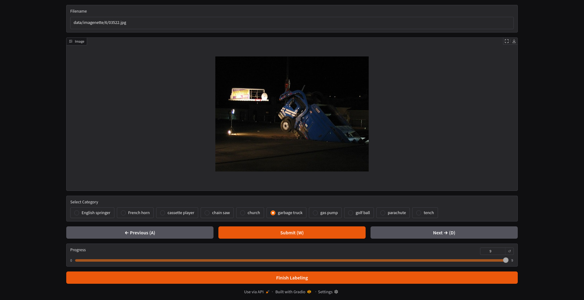
+In the UI, you can optionally run zero-shot inference on the image. This will use a VLM to predict the label of the image. There are a dozen VLM models as supported in the [x.infer project](https://github.com/dnth/x.infer).
+
+![Zero-Shot Inference](https://raw.githubusercontent.com/dnth/active-vision/main/assets/zero_shot_ui.png)
+
 Once complete, the labeled samples will be save into a new df.
 We can now add the newly labeled data to the training set.
 
@@ -167,12 +175,12 @@ The active learning loop is a iterative process and can keep going until you hit
 For this dataset,I decided to stop the active learning loop at 275 labeled images because the performance on the evaluation set is close to the top performing model on the leaderboard. 
 
 
-| #Labeled Images | Evaluation Accuracy | Train Epochs | Model                | Active Learning | Source |
-|-----------------|---------------------|--------------|----------------------|----------------|--------|
-| 9469            | 94.90%              | 80           | xse_resnext50        | ❌             | [Link](https://github.com/fastai/imagenette) |
-| 9469            | 95.11%              | 200          | xse_resnext50        | ❌             | [Link](https://github.com/fastai/imagenette) |
-| 275             | 99.33%               | 6            | convnext_small_in22k | ✓              | [Link](https://github.com/dnth/active-vision/blob/main/nbs/05_retrain_larger.ipynb) |
-| 275             | 93.40%               | 4            | resnet18             | ✓              | [Link](https://github.com/dnth/active-vision/blob/main/nbs/04_relabel_loop.ipynb) |
+| #Labeled Images 	| Evaluation Accuracy 	| Train Epochs 	| Model                	| Active Learning 	| Source                                                                              	|
+|----------------:	|--------------------:	|-------------:	|----------------------	|:---------------:	|-------------------------------------------------------------------------------------	|
+| 9469            	| 94.90%              	| 80           	| xse_resnext50        	| ❌                | [Link](https://github.com/fastai/imagenette)                                        	 |
+| 9469            	| 95.11%              	| 200          	| xse_resnext50        	| ❌                | [Link](https://github.com/fastai/imagenette)                                        	 |
+| 275             	| 99.33%              	| 6            	| convnext_small_in22k 	| ✓               	| [Link](https://github.com/dnth/active-vision/blob/main/nbs/05_retrain_larger.ipynb) 	|
+| 275             	| 93.40%              	| 4            	| resnet18             	| ✓               	| [Link](https://github.com/dnth/active-vision/blob/main/nbs/04_relabel_loop.ipynb)   	|
 
 ### Dog Food
 - num classes: 2
@@ -182,11 +190,11 @@ To start the active learning loop, I labeled 20 images (10 images from each clas
 
 I decided to stop the active learning loop at 160 labeled images because the performance on the evaluation set is close to the top performing model on the leaderboard. You can decide your own stopping point based on your use case.
 
-| #Labeled Images | Evaluation Accuracy | Train Epochs | Model | Active Learning | Source |
-|-----------------|---------------------|--------------|-------|----------------|--------|
-| 2100            | 99.70%              | ?            | vit-base-patch16-224   | ❌             | [Link](https://huggingface.co/abhishek/autotrain-dog-vs-food) |
-| 160             | 100.00%             | 6            | convnext_small_in22k   | ✓              | [Link](https://github.com/dnth/active-vision/blob/main/nbs/dog_food_dataset/02_train.ipynb) |
-| 160             | 97.60%              | 4            | resnet18              | ✓              | [Link](https://github.com/dnth/active-vision/blob/main/nbs/dog_food_dataset/01_label.ipynb) |
+| #Labeled Images 	| Evaluation Accuracy 	| Train Epochs 	| Model                	| Active Learning 	| Source                                                                                      	|
+|----------------:	|--------------------:	|-------------:	|----------------------	|:---------------:	|---------------------------------------------------------------------------------------------	|
+| 2100            	| 99.70%              	| ?            	| vit-base-patch16-224 	| ❌               	| [Link](https://huggingface.co/abhishek/autotrain-dog-vs-food)                               	|
+| 160             	| 100.00%             	| 6            	| convnext_small_in22k 	| ✓               	| [Link](https://github.com/dnth/active-vision/blob/main/nbs/dog_food_dataset/02_train.ipynb) 	|
+| 160             	| 97.60%              	| 4            	| resnet18             	| ✓               	| [Link](https://github.com/dnth/active-vision/blob/main/nbs/dog_food_dataset/01_label.ipynb) 	|
 
 ### Oxford-IIIT Pet
 - num classes: 37
@@ -196,13 +204,27 @@ To start the active learning loop, I labeled 370 images (10 images from each cla
 
 I decided to stop the active learning loop at 612 labeled images because the performance on the evaluation set is close to the top performing model on the leaderboard. You can decide your own stopping point based on your use case.
 
-| #Labeled Images | Evaluation Accuracy | Train Epochs | Model | Active Learning | Source |
-|-----------------|---------------------|--------------|-------|----------------|--------|
-| 3680             | 95.40%              | 5           | vit-base-patch16-224   | ❌              | [Link](https://huggingface.co/walterg777/vit-base-oxford-iiit-pets) |
-| 612             | 90.26%              | 11            | convnext_small_in22k              | ✓              | [Link](https://github.com/dnth/active-vision/blob/main/nbs/oxford_iiit_pets/02_train.ipynb) |
-| 612             | 91.38%              | 11            | vit-base-patch16-224              | ✓              | [Link](https://github.com/dnth/active-vision/blob/main/nbs/oxford_iiit_pets/03_train_vit.ipynb) |
+| #Labeled Images 	| Evaluation Accuracy 	| Train Epochs 	| Model                	| Active Learning 	| Source                                                                                          	|
+|----------------:	|--------------------:	|-------------:	|----------------------	|:---------------:	|-------------------------------------------------------------------------------------------------	|
+| 3680            	| 95.40%              	| 5            	| vit-base-patch16-224 	| ❌                | [Link](https://huggingface.co/walterg777/vit-base-oxford-iiit-pets)                             	 |
+| 612             	| 90.26%              	| 11           	| convnext_small_in22k 	| ✓               	| [Link](https://github.com/dnth/active-vision/blob/main/nbs/oxford_iiit_pets/02_train.ipynb)     	|
+| 612             	| 91.38%              	| 11           	| vit-base-patch16-224 	| ✓               	| [Link](https://github.com/dnth/active-vision/blob/main/nbs/oxford_iiit_pets/03_train_vit.ipynb) 	|
+
+### Eurosat RGB
+- num classes: 10
+- num images: 16100
+
+To start the active learning loop, I labeled 100 images (10 images from each class) and iteratively labeled the most informative images until I hit 1188 labeled images. 
+
+I decided to stop the active learning loop at 1188 labeled images because the performance on the evaluation set is close to the top performing model on the leaderboard. You can decide your own stopping point based on your use case.
 
 
+| #Labeled Images 	| Evaluation Accuracy 	| Train Epochs 	| Model                	| Active Learning 	| Source                                                                                     	|
+|----------------:	|--------------------:	|-------------:	|----------------------	|:---------------:	|--------------------------------------------------------------------------------------------	|
+| 16100           	| 98.55%              	| 6            	| vit-base-patch16-224 	| ❌                | [Link](https://github.com/dnth/active-vision/blob/main/nbs/eurosat_rgb/03_train_all.ipynb)  |
+| 1188            	| 94.59%              	| 6            	| vit-base-patch16-224 	| ✓               	| [Link](https://github.com/dnth/active-vision/blob/main/nbs/eurosat_rgb/02_train.ipynb)     	|
+| 1188            	| 96.57%              	| 13           	| vit-base-patch16-224 	| ✓               	| [Link](https://github.com/dnth/active-vision/blob/main/nbs/eurosat_rgb/02_train.ipynb)     	|
+
 
 ## ➿ Workflow
 This section describes a more detailed workflow for active learning. There are two workflows for active learning that we can use depending on the availability of labeled data.
@@ -270,55 +292,21 @@ graph TD
 
 
 
-<!-- ## Methodology
-To test out the workflows we will use the [imagenette dataset](https://huggingface.co/datasets/frgfm/imagenette). But this will be applicable to any dataset.
-
-Imagenette is a subset of the ImageNet dataset with 10 classes. We will use this dataset to test out the workflows. Additionally, Imagenette has an existing leaderboard which we can use to evaluate the performance of the models.
-
-### Step 1: Download the dataset
-Download the imagenette dataset. The imagenette dataset has a train and validation split. Since the leaderboard is based on the validation set, we will evalutate the performance of our model on the validation set to make it easier to compare to the leaderboard.
-
-We will treat the imagenette train set as a unlabeled set and iteratively sample from it while monitoring the performance on the validation set. Ideally we will be able to get to a point where the performance on the validation set is close to the leaderboard with minimal number of labeled images.
+## 🧱 Sampling Approaches
 
-I've processed the imagenette dataset and uploaded it to the hub. You can download it from [here](https://huggingface.co/datasets/dnth/active-learning-imagenette).
+Recommendation 1:
+- 10% randomly selected from unlabeled items.
+- 80% selected from the lowest confidence items.
+- 10% selected as outliers.
 
-To load the dataset, you can use the following code:
-```python
-from datasets import load_dataset
-
-unlabeled_dataset = load_dataset("dnth/active-learning-imagenette", "unlabeled")
-eval_dataset = load_dataset("dnth/active-learning-imagenette", "evaluation")
-```
+Recommendation 2:
 
-### Step 2: Initial Sampling
-Label an initial dataset of 10 images from each class. This will give us a small proxy dataset to train our model on. The sampling will be done randomly. There are more intelligent sampling strategies but we will start with random sampling.
+- Sample 100 predicted images at 10–20% confidence.
+- Sample 100 predicted images at 20–30% confidence.
+- Sample 100 predicted images at 30–40% confidence, and so on.
 
-### Step 3: Training the proxy model
-Train a proxy model on the initial dataset. The proxy model will be a small model that is easy to train and deploy. We will use the fastai framework to train the model. We will use the resnet18 architecture as a starting point. Once training is complete, compute the accuracy of the proxy model on the validation set and compare it to the leaderboard.
 
-> [!TIP]
-> With the initial model we got 91.24% accuracy on the validation set. See the [notebook](./nbs/01_initial_sampling.ipynb) for more details.
-> | Train Epochs | Number of Images | Validation Accuracy |      Source      |
-> |--------------|-----------------|----------------------|------------------|
-> | 10           | 100             | 91.24%               | Initial sampling [notebook](./nbs/01_initial_sampling.ipynb) |
-> | 80           | 9469            | 94.90%               | fastai |
-> | 200          | 9469            | 95.11%               | fastai |
+Uncertainty and diversity sampling are most effective when combined. For instance, you could first sample the most uncertain items using an uncertainty sampling method, then apply a diversity sampling method such as clustering to select a diverse set from the uncertain items.
 
+Ultimately, the right ratios can depend on the specific task and dataset.
 
-
-### Step 4: Inference on the unlabeled dataset
-Run inference on the unlabeled dataset (the remaining imagenette train set) and evaluate the performance of the proxy model. 
-
-### Step 5: Active learning
-Use active learning to select the most informative images to label from the unlabeled set. Pick the top 10 images from the unlabeled set that the proxy model is least confident about and label them.
-
-### Step 6: Repeat
-Repeat step 3 - 5 until the performance on the validation set is close to the leaderboard. Note the number of labeled images vs the performance on the validation set. Ideally we want to get to a point where the performance on the validation set is close to the leaderboard with minimal number of labeled images.
-
-
-After the first iteration we got 94.57% accuracy on the validation set. See the [notebook](./nbs/03_retrain_model.ipynb) for more details.
-
-> [!TIP]
-> | Train Epochs | Number of Images | Validation Accuracy |      Source      |
-> |--------------|-----------------|----------------------|------------------|
-> | 10           | 200             | 94.57%               | First relabeling [notebook](./nbs/03_retrain_model.ipynb) | -->

{active_vision-0.0.5 → active_vision-0.1.1}/README.md

@@ -52,17 +52,18 @@ cd active-vision
 pip install -e .
 ```
 
-I recommend using [uv](https://docs.astral.sh/uv/) to set up a virtual environment and install the package. You can also use other virtual env of your choice.
-
-If you're using uv:
-
-```bash
-uv venv
-uv sync
-```
-Once the virtual environment is created, you can install the package using pip.
 
 > [!TIP]
+> I recommend using [uv](https://docs.astral.sh/uv/) to set up a virtual environment and install the package. You can also use other virtual env of your choice.
+> 
+> If you're using uv:
+> 
+> ```bash
+> uv venv
+> uv sync
+> ```
+> Once the virtual environment is created, you can install the package using pip.
+>
 > If you're using uv add a `uv` before the pip install command to install into your virtual environment. Eg:
 > ```bash
 > uv pip install active-vision
@@ -101,12 +102,16 @@ pred_df = al.predict(filepaths)
 # Sample low confidence predictions from unlabeled set
 uncertain_df = al.sample_uncertain(pred_df, num_samples=10)
 
-# Launch a Gradio UI to label the low confidence samples
+# Launch a Gradio UI to label the low confidence samples, save the labeled samples to a file
 al.label(uncertain_df, output_filename="uncertain")
 ```
 
 ![Gradio UI](https://raw.githubusercontent.com/dnth/active-vision/main/assets/labeling_ui.png)
 
+In the UI, you can optionally run zero-shot inference on the image. This will use a VLM to predict the label of the image. There are a dozen VLM models as supported in the [x.infer project](https://github.com/dnth/x.infer).
+
+![Zero-Shot Inference](https://raw.githubusercontent.com/dnth/active-vision/main/assets/zero_shot_ui.png)
+
 Once complete, the labeled samples will be save into a new df.
 We can now add the newly labeled data to the training set.
 
@@ -151,12 +156,12 @@ The active learning loop is a iterative process and can keep going until you hit
 For this dataset,I decided to stop the active learning loop at 275 labeled images because the performance on the evaluation set is close to the top performing model on the leaderboard. 
 
 
-| #Labeled Images | Evaluation Accuracy | Train Epochs | Model                | Active Learning | Source |
-|-----------------|---------------------|--------------|----------------------|----------------|--------|
-| 9469            | 94.90%              | 80           | xse_resnext50        | ❌             | [Link](https://github.com/fastai/imagenette) |
-| 9469            | 95.11%              | 200          | xse_resnext50        | ❌             | [Link](https://github.com/fastai/imagenette) |
-| 275             | 99.33%               | 6            | convnext_small_in22k | ✓              | [Link](https://github.com/dnth/active-vision/blob/main/nbs/05_retrain_larger.ipynb) |
-| 275             | 93.40%               | 4            | resnet18             | ✓              | [Link](https://github.com/dnth/active-vision/blob/main/nbs/04_relabel_loop.ipynb) |
+| #Labeled Images 	| Evaluation Accuracy 	| Train Epochs 	| Model                	| Active Learning 	| Source                                                                              	|
+|----------------:	|--------------------:	|-------------:	|----------------------	|:---------------:	|-------------------------------------------------------------------------------------	|
+| 9469            	| 94.90%              	| 80           	| xse_resnext50        	| ❌                | [Link](https://github.com/fastai/imagenette)                                        	 |
+| 9469            	| 95.11%              	| 200          	| xse_resnext50        	| ❌                | [Link](https://github.com/fastai/imagenette)                                        	 |
+| 275             	| 99.33%              	| 6            	| convnext_small_in22k 	| ✓               	| [Link](https://github.com/dnth/active-vision/blob/main/nbs/05_retrain_larger.ipynb) 	|
+| 275             	| 93.40%              	| 4            	| resnet18             	| ✓               	| [Link](https://github.com/dnth/active-vision/blob/main/nbs/04_relabel_loop.ipynb)   	|
 
 ### Dog Food
 - num classes: 2
@@ -166,11 +171,11 @@ To start the active learning loop, I labeled 20 images (10 images from each clas
 
 I decided to stop the active learning loop at 160 labeled images because the performance on the evaluation set is close to the top performing model on the leaderboard. You can decide your own stopping point based on your use case.
 
-| #Labeled Images | Evaluation Accuracy | Train Epochs | Model | Active Learning | Source |
-|-----------------|---------------------|--------------|-------|----------------|--------|
-| 2100            | 99.70%              | ?            | vit-base-patch16-224   | ❌             | [Link](https://huggingface.co/abhishek/autotrain-dog-vs-food) |
-| 160             | 100.00%             | 6            | convnext_small_in22k   | ✓              | [Link](https://github.com/dnth/active-vision/blob/main/nbs/dog_food_dataset/02_train.ipynb) |
-| 160             | 97.60%              | 4            | resnet18              | ✓              | [Link](https://github.com/dnth/active-vision/blob/main/nbs/dog_food_dataset/01_label.ipynb) |
+| #Labeled Images 	| Evaluation Accuracy 	| Train Epochs 	| Model                	| Active Learning 	| Source                                                                                      	|
+|----------------:	|--------------------:	|-------------:	|----------------------	|:---------------:	|---------------------------------------------------------------------------------------------	|
+| 2100            	| 99.70%              	| ?            	| vit-base-patch16-224 	| ❌               	| [Link](https://huggingface.co/abhishek/autotrain-dog-vs-food)                               	|
+| 160             	| 100.00%             	| 6            	| convnext_small_in22k 	| ✓               	| [Link](https://github.com/dnth/active-vision/blob/main/nbs/dog_food_dataset/02_train.ipynb) 	|
+| 160             	| 97.60%              	| 4            	| resnet18             	| ✓               	| [Link](https://github.com/dnth/active-vision/blob/main/nbs/dog_food_dataset/01_label.ipynb) 	|
 
 ### Oxford-IIIT Pet
 - num classes: 37
@@ -180,13 +185,27 @@ To start the active learning loop, I labeled 370 images (10 images from each cla
 
 I decided to stop the active learning loop at 612 labeled images because the performance on the evaluation set is close to the top performing model on the leaderboard. You can decide your own stopping point based on your use case.
 
-| #Labeled Images | Evaluation Accuracy | Train Epochs | Model | Active Learning | Source |
-|-----------------|---------------------|--------------|-------|----------------|--------|
-| 3680             | 95.40%              | 5           | vit-base-patch16-224   | ❌              | [Link](https://huggingface.co/walterg777/vit-base-oxford-iiit-pets) |
-| 612             | 90.26%              | 11            | convnext_small_in22k              | ✓              | [Link](https://github.com/dnth/active-vision/blob/main/nbs/oxford_iiit_pets/02_train.ipynb) |
-| 612             | 91.38%              | 11            | vit-base-patch16-224              | ✓              | [Link](https://github.com/dnth/active-vision/blob/main/nbs/oxford_iiit_pets/03_train_vit.ipynb) |
+| #Labeled Images 	| Evaluation Accuracy 	| Train Epochs 	| Model                	| Active Learning 	| Source                                                                                          	|
+|----------------:	|--------------------:	|-------------:	|----------------------	|:---------------:	|-------------------------------------------------------------------------------------------------	|
+| 3680            	| 95.40%              	| 5            	| vit-base-patch16-224 	| ❌                | [Link](https://huggingface.co/walterg777/vit-base-oxford-iiit-pets)                             	 |
+| 612             	| 90.26%              	| 11           	| convnext_small_in22k 	| ✓               	| [Link](https://github.com/dnth/active-vision/blob/main/nbs/oxford_iiit_pets/02_train.ipynb)     	|
+| 612             	| 91.38%              	| 11           	| vit-base-patch16-224 	| ✓               	| [Link](https://github.com/dnth/active-vision/blob/main/nbs/oxford_iiit_pets/03_train_vit.ipynb) 	|
+
+### Eurosat RGB
+- num classes: 10
+- num images: 16100
+
+To start the active learning loop, I labeled 100 images (10 images from each class) and iteratively labeled the most informative images until I hit 1188 labeled images. 
+
+I decided to stop the active learning loop at 1188 labeled images because the performance on the evaluation set is close to the top performing model on the leaderboard. You can decide your own stopping point based on your use case.
 
 
+| #Labeled Images 	| Evaluation Accuracy 	| Train Epochs 	| Model                	| Active Learning 	| Source                                                                                     	|
+|----------------:	|--------------------:	|-------------:	|----------------------	|:---------------:	|--------------------------------------------------------------------------------------------	|
+| 16100           	| 98.55%              	| 6            	| vit-base-patch16-224 	| ❌                | [Link](https://github.com/dnth/active-vision/blob/main/nbs/eurosat_rgb/03_train_all.ipynb)  |
+| 1188            	| 94.59%              	| 6            	| vit-base-patch16-224 	| ✓               	| [Link](https://github.com/dnth/active-vision/blob/main/nbs/eurosat_rgb/02_train.ipynb)     	|
+| 1188            	| 96.57%              	| 13           	| vit-base-patch16-224 	| ✓               	| [Link](https://github.com/dnth/active-vision/blob/main/nbs/eurosat_rgb/02_train.ipynb)     	|
+
 
 ## ➿ Workflow
 This section describes a more detailed workflow for active learning. There are two workflows for active learning that we can use depending on the availability of labeled data.
@@ -254,55 +273,21 @@ graph TD
 
 
 
-<!-- ## Methodology
-To test out the workflows we will use the [imagenette dataset](https://huggingface.co/datasets/frgfm/imagenette). But this will be applicable to any dataset.
-
-Imagenette is a subset of the ImageNet dataset with 10 classes. We will use this dataset to test out the workflows. Additionally, Imagenette has an existing leaderboard which we can use to evaluate the performance of the models.
-
-### Step 1: Download the dataset
-Download the imagenette dataset. The imagenette dataset has a train and validation split. Since the leaderboard is based on the validation set, we will evalutate the performance of our model on the validation set to make it easier to compare to the leaderboard.
-
-We will treat the imagenette train set as a unlabeled set and iteratively sample from it while monitoring the performance on the validation set. Ideally we will be able to get to a point where the performance on the validation set is close to the leaderboard with minimal number of labeled images.
+## 🧱 Sampling Approaches
 
-I've processed the imagenette dataset and uploaded it to the hub. You can download it from [here](https://huggingface.co/datasets/dnth/active-learning-imagenette).
+Recommendation 1:
+- 10% randomly selected from unlabeled items.
+- 80% selected from the lowest confidence items.
+- 10% selected as outliers.
 
-To load the dataset, you can use the following code:
-```python
-from datasets import load_dataset
-
-unlabeled_dataset = load_dataset("dnth/active-learning-imagenette", "unlabeled")
-eval_dataset = load_dataset("dnth/active-learning-imagenette", "evaluation")
-```
+Recommendation 2:
 
-### Step 2: Initial Sampling
-Label an initial dataset of 10 images from each class. This will give us a small proxy dataset to train our model on. The sampling will be done randomly. There are more intelligent sampling strategies but we will start with random sampling.
+- Sample 100 predicted images at 10–20% confidence.
+- Sample 100 predicted images at 20–30% confidence.
+- Sample 100 predicted images at 30–40% confidence, and so on.
 
-### Step 3: Training the proxy model
-Train a proxy model on the initial dataset. The proxy model will be a small model that is easy to train and deploy. We will use the fastai framework to train the model. We will use the resnet18 architecture as a starting point. Once training is complete, compute the accuracy of the proxy model on the validation set and compare it to the leaderboard.
 
-> [!TIP]
-> With the initial model we got 91.24% accuracy on the validation set. See the [notebook](./nbs/01_initial_sampling.ipynb) for more details.
-> | Train Epochs | Number of Images | Validation Accuracy |      Source      |
-> |--------------|-----------------|----------------------|------------------|
-> | 10           | 100             | 91.24%               | Initial sampling [notebook](./nbs/01_initial_sampling.ipynb) |
-> | 80           | 9469            | 94.90%               | fastai |
-> | 200          | 9469            | 95.11%               | fastai |
+Uncertainty and diversity sampling are most effective when combined. For instance, you could first sample the most uncertain items using an uncertainty sampling method, then apply a diversity sampling method such as clustering to select a diverse set from the uncertain items.
 
+Ultimately, the right ratios can depend on the specific task and dataset.
 
-
-### Step 4: Inference on the unlabeled dataset
-Run inference on the unlabeled dataset (the remaining imagenette train set) and evaluate the performance of the proxy model. 
-
-### Step 5: Active learning
-Use active learning to select the most informative images to label from the unlabeled set. Pick the top 10 images from the unlabeled set that the proxy model is least confident about and label them.
-
-### Step 6: Repeat
-Repeat step 3 - 5 until the performance on the validation set is close to the leaderboard. Note the number of labeled images vs the performance on the validation set. Ideally we want to get to a point where the performance on the validation set is close to the leaderboard with minimal number of labeled images.
-
-
-After the first iteration we got 94.57% accuracy on the validation set. See the [notebook](./nbs/03_retrain_model.ipynb) for more details.
-
-> [!TIP]
-> | Train Epochs | Number of Images | Validation Accuracy |      Source      |
-> |--------------|-----------------|----------------------|------------------|
-> | 10           | 200             | 94.57%               | First relabeling [notebook](./nbs/03_retrain_model.ipynb) | -->

{active_vision-0.0.5 → active_vision-0.1.1}/pyproject.toml

@@ -1,10 +1,11 @@
 [project]
 name = "active-vision"
-version = "0.0.5"
+version = "0.1.1"
 description = "Active learning for edge vision."
 readme = "README.md"
 requires-python = ">=3.10"
 dependencies = [
+    "accelerate>=1.2.1",
     "datasets>=3.2.0",
     "fastai>=2.7.18",
     "gradio>=5.12.0",
@@ -13,4 +14,6 @@ dependencies = [
     "loguru>=0.7.3",
     "seaborn>=0.13.2",
     "timm>=1.0.13",
+    "transformers>=4.48.0",
+    "xinfer>=0.3.2",
 ]

active_vision-0.1.1/src/active_vision/__init__.py

@@ -0,0 +1,3 @@
+__version__ = "0.1.1"
+
+from .core import *