PySDKit 0.4__tar.gz → 0.4.2__tar.gz
This diff represents the content of publicly available package versions that have been released to one of the supported registries. The information contained in this diff is provided for informational purposes only and reflects changes between package versions as they appear in their respective public registries.
- {PySDKit-0.4 → PySDKit-0.4.2}/PKG-INFO +5 -8
- {PySDKit-0.4 → PySDKit-0.4.2}/PySDKit.egg-info/PKG-INFO +5 -8
- {PySDKit-0.4 → PySDKit-0.4.2}/PySDKit.egg-info/SOURCES.txt +1 -1
- {PySDKit-0.4 → PySDKit-0.4.2}/README.md +4 -7
- {PySDKit-0.4 → PySDKit-0.4.2}/pysdkit/__init__.py +1 -1
- {PySDKit-0.4 → PySDKit-0.4.2}/pysdkit/emd/EMD.py +2 -1
- PySDKit-0.4.2/pysdkit/ewt/__init__.py +2 -0
- PySDKit-0.4.2/pysdkit/ewt/ewt.py +500 -0
- PySDKit-0.4.2/pysdkit/utils/__init__.py +35 -0
- {PySDKit-0.4 → PySDKit-0.4.2}/pysdkit/vmd/_vmd_c.py +3 -5
- {PySDKit-0.4 → PySDKit-0.4.2}/pysdkit/vmd/_vmd_f.py +2 -3
- {PySDKit-0.4 → PySDKit-0.4.2}/setup.py +1 -1
- PySDKit-0.4/pysdkit/ewt/__init__.py +0 -2
- PySDKit-0.4/pysdkit/ewt/_ewt.py +0 -449
- PySDKit-0.4/pysdkit/utils/__init__.py +0 -34
- {PySDKit-0.4 → PySDKit-0.4.2}/LICENSE +0 -0
- {PySDKit-0.4 → PySDKit-0.4.2}/PySDKit.egg-info/dependency_links.txt +0 -0
- {PySDKit-0.4 → PySDKit-0.4.2}/PySDKit.egg-info/requires.txt +0 -0
- {PySDKit-0.4 → PySDKit-0.4.2}/PySDKit.egg-info/top_level.txt +0 -0
- {PySDKit-0.4 → PySDKit-0.4.2}/pysdkit/data/__init__.py +0 -0
- {PySDKit-0.4 → PySDKit-0.4.2}/pysdkit/data/_add_noise.py +0 -0
- {PySDKit-0.4 → PySDKit-0.4.2}/pysdkit/data/_generator.py +0 -0
- {PySDKit-0.4 → PySDKit-0.4.2}/pysdkit/emd/BEMD.py +0 -0
- {PySDKit-0.4 → PySDKit-0.4.2}/pysdkit/emd/__init__.py +0 -0
- {PySDKit-0.4 → PySDKit-0.4.2}/pysdkit/emd/_find_extrema.py +0 -0
- {PySDKit-0.4 → PySDKit-0.4.2}/pysdkit/emd/_prepare_points.py +0 -0
- {PySDKit-0.4 → PySDKit-0.4.2}/pysdkit/emd/_splines.py +0 -0
- {PySDKit-0.4 → PySDKit-0.4.2}/pysdkit/emd2d/__init__.py +0 -0
- {PySDKit-0.4 → PySDKit-0.4.2}/pysdkit/metrics/_Index_of_Orthogonality.py +0 -0
- {PySDKit-0.4 → PySDKit-0.4.2}/pysdkit/metrics/__init__.py +0 -0
- {PySDKit-0.4 → PySDKit-0.4.2}/pysdkit/plot/__init__.py +0 -0
- {PySDKit-0.4 → PySDKit-0.4.2}/pysdkit/plot/_fourier_spectra.py +0 -0
- {PySDKit-0.4 → PySDKit-0.4.2}/pysdkit/plot/_functions.py +0 -0
- {PySDKit-0.4 → PySDKit-0.4.2}/pysdkit/plot/_plot_imfs.py +0 -0
- {PySDKit-0.4 → PySDKit-0.4.2}/pysdkit/plot/main.py +0 -0
- {PySDKit-0.4 → PySDKit-0.4.2}/pysdkit/utils/_differ.py +0 -0
- {PySDKit-0.4 → PySDKit-0.4.2}/pysdkit/utils/_fft.py +0 -0
- {PySDKit-0.4 → PySDKit-0.4.2}/pysdkit/utils/_function.py +0 -0
- {PySDKit-0.4 → PySDKit-0.4.2}/pysdkit/utils/_smooth1d.py +0 -0
- {PySDKit-0.4 → PySDKit-0.4.2}/pysdkit/utils/hilbert.py +0 -0
- {PySDKit-0.4 → PySDKit-0.4.2}/pysdkit/utils/mirror.py +0 -0
- {PySDKit-0.4 → PySDKit-0.4.2}/pysdkit/utils/process.py +0 -0
- {PySDKit-0.4 → PySDKit-0.4.2}/pysdkit/vmd/__init__.py +0 -0
- {PySDKit-0.4 → PySDKit-0.4.2}/pysdkit/vmd/_avmd.py +0 -0
- {PySDKit-0.4 → PySDKit-0.4.2}/pysdkit/vmd/_mvmd.py +0 -0
- {PySDKit-0.4 → PySDKit-0.4.2}/pysdkit/vmd/_svmd.py +0 -0
- {PySDKit-0.4 → PySDKit-0.4.2}/pysdkit/vmd/base.py +0 -0
- {PySDKit-0.4 → PySDKit-0.4.2}/pysdkit/vncmd/__init__.py +0 -0
- {PySDKit-0.4 → PySDKit-0.4.2}/pysdkit/vncmd/vncmd.py +0 -0
- {PySDKit-0.4 → PySDKit-0.4.2}/setup.cfg +0 -0
|
@@ -1,6 +1,6 @@
|
|
|
1
1
|
Metadata-Version: 2.1
|
|
2
2
|
Name: PySDKit
|
|
3
|
-
Version: 0.4
|
|
3
|
+
Version: 0.4.2
|
|
4
4
|
Summary: A Python library for signal decomposition algorithms with a unified interface
|
|
5
5
|
Home-page: https://github.com/wwhenxuan/PySDKit
|
|
6
6
|
Author: whenxuan
|
|
@@ -28,9 +28,7 @@ License-File: LICENSE
|
|
|
28
28
|
|
|
29
29
|
A Python library for signal decomposition algorithms
|
|
30
30
|
|
|
31
|
-
|
|
32
|
-
<img src=".\images\Logo_sd.png" alt="Logo_sd" width="500"/>
|
|
33
|
-
</div>
|
|
31
|
+
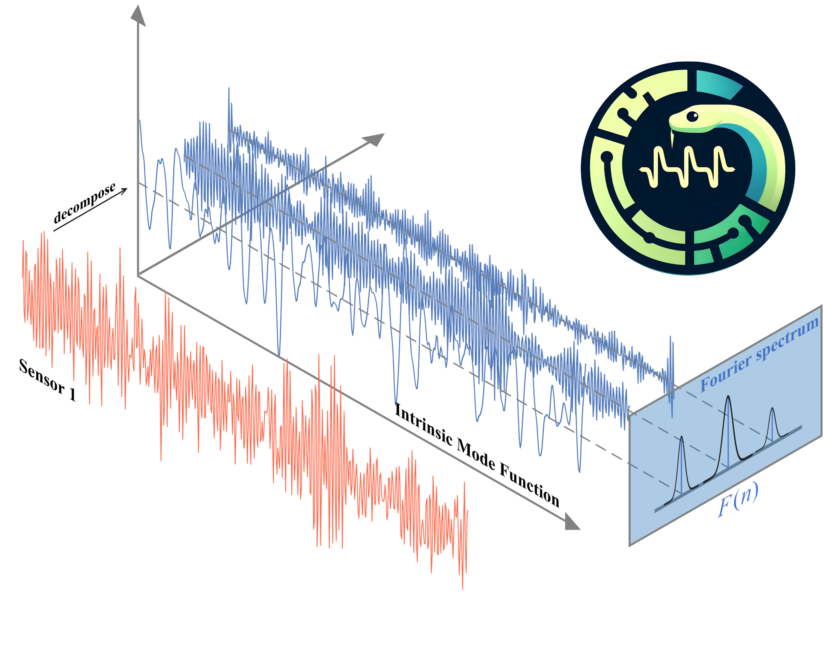
|
|
34
32
|
|
|
35
33
|
## Installation
|
|
36
34
|
|
|
@@ -64,7 +62,7 @@ IMFs = emd.fit_transform(signal, max_imf=2)
|
|
|
64
62
|
plot_IMFs(signal, IMFs)
|
|
65
63
|
~~~
|
|
66
64
|
|
|
67
|
-
|
|
65
|
+
|
|
68
66
|
|
|
69
67
|
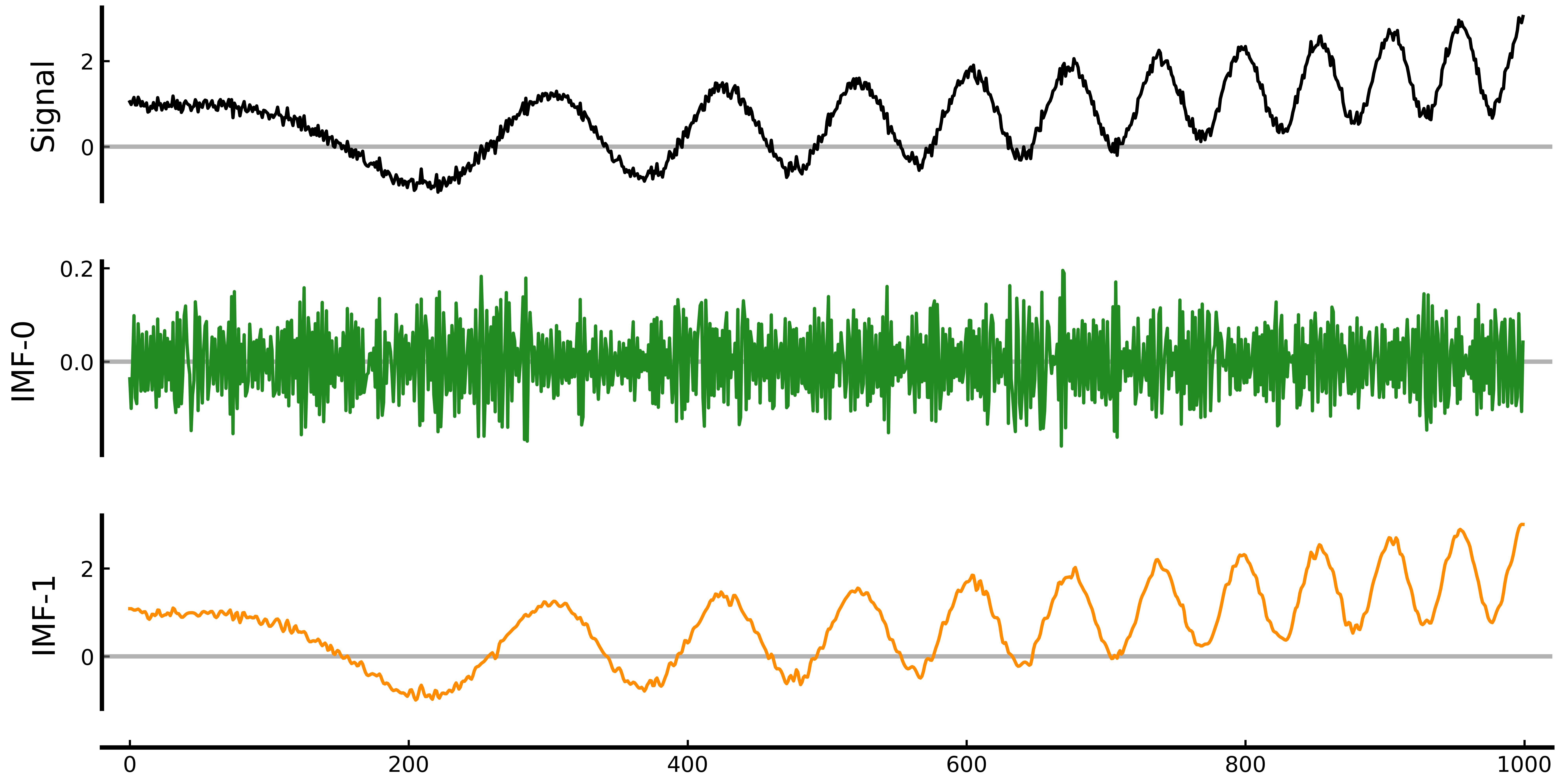
The EMD in the above example is the most classic `empirical mode decomposition` algorithm in signal decomposition. For more complex signals, you can try other algorithms such as variational mode decomposition ([`VMD`](https://ieeexplore.ieee.org/abstract/document/6655981)).
|
|
70
68
|
|
|
@@ -82,7 +80,7 @@ print(IMFs.shape)
|
|
|
82
80
|
vmd.plot_IMFs(save_figure=True)
|
|
83
81
|
~~~
|
|
84
82
|
|
|
85
|
-
|
|
83
|
+
|
|
86
84
|
|
|
87
85
|
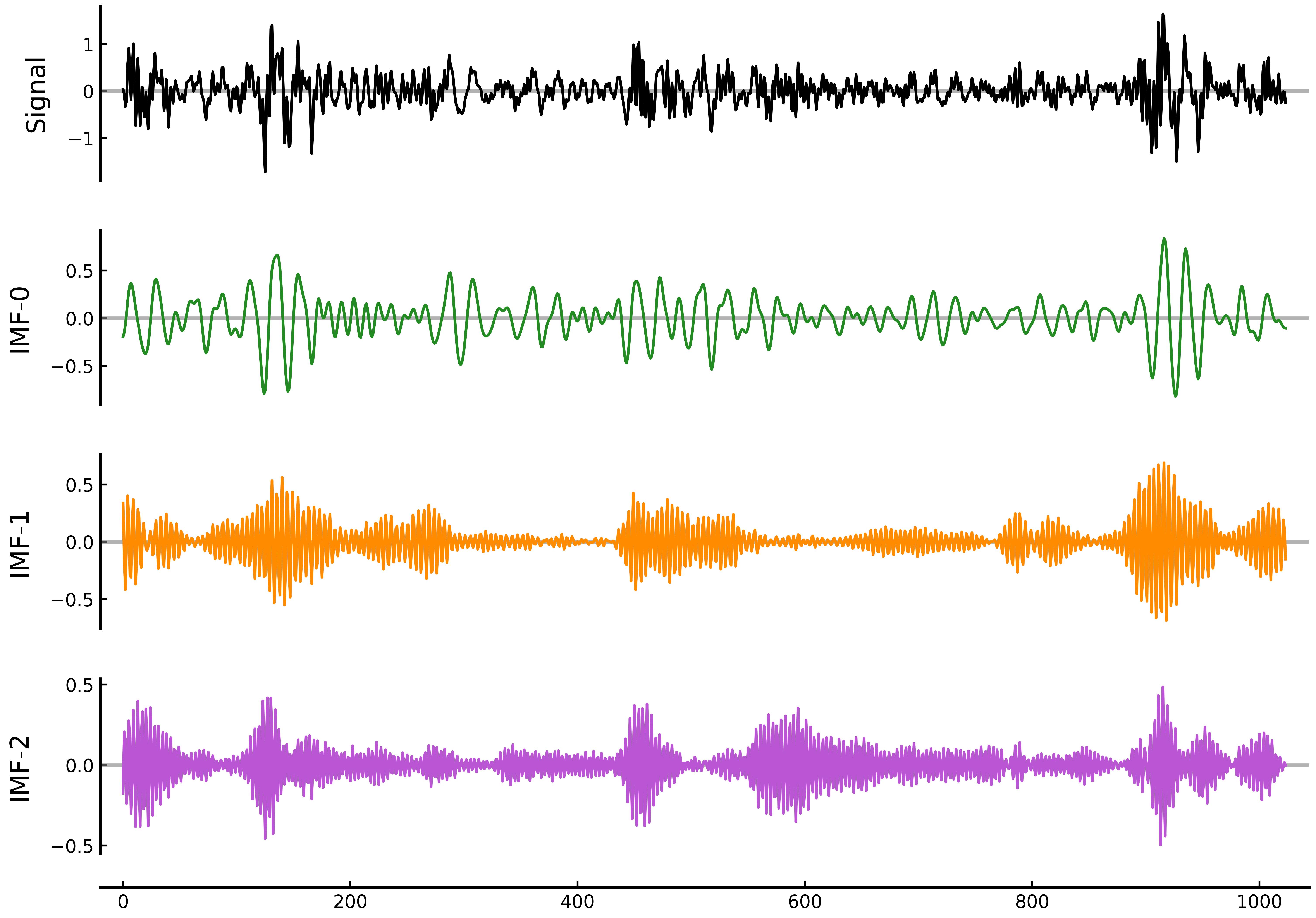
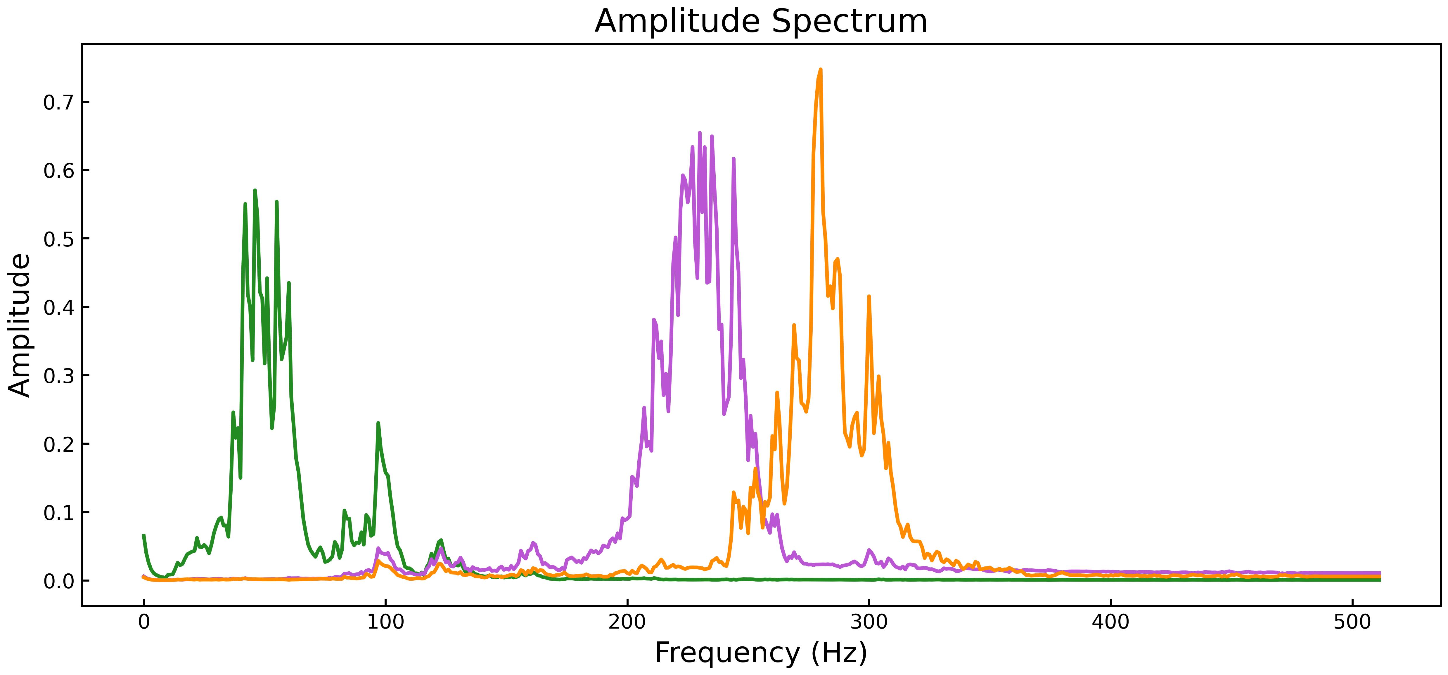
Better observe the characteristics of the decomposed intrinsic mode function in the frequency domain.
|
|
88
86
|
|
|
@@ -93,5 +91,4 @@ from pysdkit.plot import plot_IMFs_amplitude_spectra
|
|
|
93
91
|
plot_IMFs_amplitude_spectra(IMFs, smooth="exp") # use exp smooth
|
|
94
92
|
~~~
|
|
95
93
|
|
|
96
|
-
|
|
97
|
-
|
|
94
|
+
|
|
@@ -1,6 +1,6 @@
|
|
|
1
1
|
Metadata-Version: 2.1
|
|
2
2
|
Name: PySDKit
|
|
3
|
-
Version: 0.4
|
|
3
|
+
Version: 0.4.2
|
|
4
4
|
Summary: A Python library for signal decomposition algorithms with a unified interface
|
|
5
5
|
Home-page: https://github.com/wwhenxuan/PySDKit
|
|
6
6
|
Author: whenxuan
|
|
@@ -28,9 +28,7 @@ License-File: LICENSE
|
|
|
28
28
|
|
|
29
29
|
A Python library for signal decomposition algorithms
|
|
30
30
|
|
|
31
|
-
|
|
32
|
-
<img src=".\images\Logo_sd.png" alt="Logo_sd" width="500"/>
|
|
33
|
-
</div>
|
|
31
|
+

|
|
34
32
|
|
|
35
33
|
## Installation
|
|
36
34
|
|
|
@@ -64,7 +62,7 @@ IMFs = emd.fit_transform(signal, max_imf=2)
|
|
|
64
62
|
plot_IMFs(signal, IMFs)
|
|
65
63
|
~~~
|
|
66
64
|
|
|
67
|
-
|
|
65
|
+

|
|
68
66
|
|
|
69
67
|
The EMD in the above example is the most classic `empirical mode decomposition` algorithm in signal decomposition. For more complex signals, you can try other algorithms such as variational mode decomposition ([`VMD`](https://ieeexplore.ieee.org/abstract/document/6655981)).
|
|
70
68
|
|
|
@@ -82,7 +80,7 @@ print(IMFs.shape)
|
|
|
82
80
|
vmd.plot_IMFs(save_figure=True)
|
|
83
81
|
~~~
|
|
84
82
|
|
|
85
|
-
|
|
83
|
+

|
|
86
84
|
|
|
87
85
|
Better observe the characteristics of the decomposed intrinsic mode function in the frequency domain.
|
|
88
86
|
|
|
@@ -93,5 +91,4 @@ from pysdkit.plot import plot_IMFs_amplitude_spectra
|
|
|
93
91
|
plot_IMFs_amplitude_spectra(IMFs, smooth="exp") # use exp smooth
|
|
94
92
|
~~~
|
|
95
93
|
|
|
96
|
-
|
|
97
|
-
|
|
94
|
+

|
|
@@ -18,7 +18,7 @@ pysdkit/emd/_prepare_points.py
|
|
|
18
18
|
pysdkit/emd/_splines.py
|
|
19
19
|
pysdkit/emd2d/__init__.py
|
|
20
20
|
pysdkit/ewt/__init__.py
|
|
21
|
-
pysdkit/ewt/
|
|
21
|
+
pysdkit/ewt/ewt.py
|
|
22
22
|
pysdkit/metrics/_Index_of_Orthogonality.py
|
|
23
23
|
pysdkit/metrics/__init__.py
|
|
24
24
|
pysdkit/plot/__init__.py
|
|
@@ -5,9 +5,7 @@
|
|
|
5
5
|
|
|
6
6
|
A Python library for signal decomposition algorithms
|
|
7
7
|
|
|
8
|
-
|
|
9
|
-
<img src=".\images\Logo_sd.png" alt="Logo_sd" width="500"/>
|
|
10
|
-
</div>
|
|
8
|
+

|
|
11
9
|
|
|
12
10
|
## Installation
|
|
13
11
|
|
|
@@ -41,7 +39,7 @@ IMFs = emd.fit_transform(signal, max_imf=2)
|
|
|
41
39
|
plot_IMFs(signal, IMFs)
|
|
42
40
|
~~~
|
|
43
41
|
|
|
44
|
-
|
|
42
|
+

|
|
45
43
|
|
|
46
44
|
The EMD in the above example is the most classic `empirical mode decomposition` algorithm in signal decomposition. For more complex signals, you can try other algorithms such as variational mode decomposition ([`VMD`](https://ieeexplore.ieee.org/abstract/document/6655981)).
|
|
47
45
|
|
|
@@ -59,7 +57,7 @@ print(IMFs.shape)
|
|
|
59
57
|
vmd.plot_IMFs(save_figure=True)
|
|
60
58
|
~~~
|
|
61
59
|
|
|
62
|
-
|
|
60
|
+

|
|
63
61
|
|
|
64
62
|
Better observe the characteristics of the decomposed intrinsic mode function in the frequency domain.
|
|
65
63
|
|
|
@@ -70,5 +68,4 @@ from pysdkit.plot import plot_IMFs_amplitude_spectra
|
|
|
70
68
|
plot_IMFs_amplitude_spectra(IMFs, smooth="exp") # use exp smooth
|
|
71
69
|
~~~
|
|
72
70
|
|
|
73
|
-
|
|
74
|
-
|
|
71
|
+

|
|
@@ -449,8 +449,9 @@ class EMD(object):
|
|
|
449
449
|
|
|
450
450
|
if __name__ == '__main__':
|
|
451
451
|
from matplotlib import pyplot as plt
|
|
452
|
+
|
|
452
453
|
x = np.linspace(0, 1, 1024)
|
|
453
454
|
f = np.cos(22 * np.pi * x ** 2) + 6 * x ** 2
|
|
454
455
|
emd = EMD(spline_kind="akima")
|
|
455
456
|
IMFs = emd.fit_transform(f, max_imf=2)
|
|
456
|
-
print(IMFs.shape)
|
|
457
|
+
print(IMFs.shape)
|
|
@@ -0,0 +1,500 @@
|
|
|
1
|
+
# -*- coding: utf-8 -*-
|
|
2
|
+
"""
|
|
3
|
+
Created on 2024/7/12 13:41
|
|
4
|
+
@author: Whenxuan Wang
|
|
5
|
+
@email: wwhenxuan@gmail.com
|
|
6
|
+
Empirical Wavelet Transform for 1D signals
|
|
7
|
+
Original paper:
|
|
8
|
+
Gilles, J., 2013. Empirical Wavelet Transform. IEEE Transactions on Signal Processing, 61(16), pp.3999–4010.
|
|
9
|
+
Available at: http://ieeexplore.ieee.org/lpdocs/epic03/wrapper.htm?arnumber=6522142.
|
|
10
|
+
Original Matlab toolbox: https://www.mathworks.com/matlabcentral/fileexchange/42141-empirical-wavelet-transforms
|
|
11
|
+
Original Code from: https://github.com/vrcarva/ewtpy
|
|
12
|
+
"""
|
|
13
|
+
import numpy as np
|
|
14
|
+
from scipy.ndimage.filters import gaussian_filter
|
|
15
|
+
from typing import Optional
|
|
16
|
+
|
|
17
|
+
|
|
18
|
+
class EWT(object):
|
|
19
|
+
"""Empirical Wavelet Transform with Class Interface."""
|
|
20
|
+
|
|
21
|
+
def __init__(self,
|
|
22
|
+
N: Optional[int] = 5,
|
|
23
|
+
log: Optional[float] = 0,
|
|
24
|
+
detect: Optional[str] = "locmax",
|
|
25
|
+
completion: Optional[float] = 0,
|
|
26
|
+
reg: Optional[str] = 'average',
|
|
27
|
+
lengthFilter: Optional[float] = 10,
|
|
28
|
+
sigmaFilter: Optional[float] = 5) -> None:
|
|
29
|
+
"""
|
|
30
|
+
:param N: Maximum number of modes (signal components) to detect and extract.
|
|
31
|
+
:param log: Set to 0 or 1 to indicate whether to operate in the logarithmic spectrum.
|
|
32
|
+
:param detect: Method for detecting boundaries in the Fourier domain ('locmax' or other detection methods).
|
|
33
|
+
:param completion: Set to 0 or 1 to indicate whether to complete the number of modes to N if fewer are detected.
|
|
34
|
+
:param reg: Regularization method applied to the filter bank ('none', 'gaussian', or 'average').
|
|
35
|
+
:param lengthFilter: Width of the filters used in regularization (for Gaussian or average filters).
|
|
36
|
+
:param sigmaFilter: Standard deviation for the Gaussian filter in the regularization step.
|
|
37
|
+
"""
|
|
38
|
+
self.N = N
|
|
39
|
+
self.log = log
|
|
40
|
+
self.detect = detect
|
|
41
|
+
self.completion = completion
|
|
42
|
+
self.reg = reg
|
|
43
|
+
self.lengthFilter = lengthFilter
|
|
44
|
+
self.sigmaFilter = sigmaFilter
|
|
45
|
+
|
|
46
|
+
def fit_transform(self, signal: np.ndarray, N: Optional[int] = None, return_all: Optional[bool] = False):
|
|
47
|
+
"""
|
|
48
|
+
Perform Empirical Wavelet Transform on the input signal.
|
|
49
|
+
|
|
50
|
+
:param signal: Input signal array to be decomposed.
|
|
51
|
+
:param N: Number of modes to extract. Defaults to the value specified during initialization.
|
|
52
|
+
:param return_all: If True, return the EWT decomposition, the filter bank, and the boundaries.
|
|
53
|
+
If False, return only the EWT decomposition.
|
|
54
|
+
|
|
55
|
+
:returns:
|
|
56
|
+
- ewt: The extracted modes from the signal.
|
|
57
|
+
- mfb: The filter bank applied in the Fourier domain (only if return_all is True).
|
|
58
|
+
- boundaries: Boundaries detected in the Fourier spectrum (only if return_all is True).
|
|
59
|
+
"""
|
|
60
|
+
N = self.N if N is None else N
|
|
61
|
+
# Compute the one-sided magnitude of the signal's Fourier transform
|
|
62
|
+
signal_ff = np.fft.fft(signal)
|
|
63
|
+
signal_ff = abs(signal_ff[0:int(np.ceil(signal_ff.size / 2))]) # one-sided magnitude
|
|
64
|
+
|
|
65
|
+
# Detect boundaries in the Fourier domain
|
|
66
|
+
boundaries = EWT_Boundaries_Detect(signal_ff, self.log, self.detect, N, self.reg,
|
|
67
|
+
self.lengthFilter, self.sigmaFilter)
|
|
68
|
+
boundaries = boundaries * np.pi / round(signal_ff.size)
|
|
69
|
+
|
|
70
|
+
# If fewer boundaries are detected, complete to reach N-1 if completion is enabled
|
|
71
|
+
if self.completion == 1 and len(boundaries) < N - 1:
|
|
72
|
+
boundaries = EWT_Boundaries_Completion(boundaries, N - 1)
|
|
73
|
+
|
|
74
|
+
# Extend the signal by mirroring to avoid boundary effects during filtering
|
|
75
|
+
ltemp = int(np.ceil(signal.size / 2))
|
|
76
|
+
fMirr = fmirror(ts=signal, sym=ltemp, end=1)
|
|
77
|
+
ffMirr = np.fft.fft(fMirr)
|
|
78
|
+
|
|
79
|
+
# Build the filter bank based on the detected boundaries
|
|
80
|
+
mfb = EWT_Meyer_FilterBank(boundaries, ffMirr.size)
|
|
81
|
+
|
|
82
|
+
# Filter the signal to extract each subband
|
|
83
|
+
ewt = np.zeros(mfb.shape)
|
|
84
|
+
for k in range(mfb.shape[1]):
|
|
85
|
+
ewt[:, k] = np.real(np.fft.ifft(np.conjugate(mfb[:, k]) * ffMirr))
|
|
86
|
+
ewt = ewt[ltemp - 1:-ltemp, :].T
|
|
87
|
+
|
|
88
|
+
# Return the requested data
|
|
89
|
+
if return_all is True:
|
|
90
|
+
return ewt, mfb, boundaries
|
|
91
|
+
else:
|
|
92
|
+
return ewt
|
|
93
|
+
|
|
94
|
+
|
|
95
|
+
def ewt(signal, N: Optional[int] = 5,
|
|
96
|
+
log: Optional[float] = 0,
|
|
97
|
+
detect: Optional[str] = "locmax",
|
|
98
|
+
completion: Optional[float] = 0,
|
|
99
|
+
reg: Optional[str] = 'average',
|
|
100
|
+
lengthFilter: Optional[float] = 10,
|
|
101
|
+
sigmaFilter: Optional[float] = 5,
|
|
102
|
+
return_all: Optional[bool] = False):
|
|
103
|
+
"""
|
|
104
|
+
Empirical Wavelet Transform with Function Interface.
|
|
105
|
+
|
|
106
|
+
:param signal: The input signal to be decomposed.
|
|
107
|
+
:param N: Maximum number of modes (signal components) to detect and extract.
|
|
108
|
+
:param log: Set to 0 or 1 to indicate whether to work with the logarithmic spectrum.
|
|
109
|
+
:param detect: Method for detecting boundaries in the Fourier domain ('locmax' or other methods).
|
|
110
|
+
:param completion: Set to 0 or 1 to indicate whether to complete the number of modes to N if fewer are detected.
|
|
111
|
+
:param reg: Regularization method applied to the filter bank ('none', 'gaussian', or 'average').
|
|
112
|
+
:param lengthFilter: Width of the filters used in regularization (for Gaussian or average filters).
|
|
113
|
+
:param sigmaFilter: Standard deviation for the Gaussian filter in the regularization step.
|
|
114
|
+
:param return_all: If True, return the EWT decomposition, the filter bank, and the boundaries.
|
|
115
|
+
If False, return only the EWT decomposition.
|
|
116
|
+
|
|
117
|
+
:returns:
|
|
118
|
+
- ewt: The extracted modes from the signal.
|
|
119
|
+
- mfb: The filter bank in the Fourier domain (only if return_all is True).
|
|
120
|
+
- boundaries: Boundaries detected in the Fourier spectrum (only if return_all is True).
|
|
121
|
+
"""
|
|
122
|
+
# Compute the one-sided magnitude of the signal's Fourier transform
|
|
123
|
+
ff = np.fft.fft(signal)
|
|
124
|
+
ff = abs(ff[0:int(np.ceil(ff.size / 2))]) # one-sided magnitude
|
|
125
|
+
|
|
126
|
+
# Detect boundaries in the Fourier domain
|
|
127
|
+
boundaries = EWT_Boundaries_Detect(ff, log, detect, N, reg, lengthFilter, sigmaFilter)
|
|
128
|
+
boundaries = boundaries * np.pi / round(ff.size)
|
|
129
|
+
|
|
130
|
+
# If fewer boundaries are detected, complete to reach N-1 if completion is enabled
|
|
131
|
+
if completion == 1 and len(boundaries) < N - 1:
|
|
132
|
+
boundaries = EWT_Boundaries_Completion(boundaries, N - 1)
|
|
133
|
+
|
|
134
|
+
# Extend the signal by mirroring to avoid boundary effects during filtering
|
|
135
|
+
ltemp = int(np.ceil(signal.size / 2)) # Similar to MATLAB's round function
|
|
136
|
+
fMirr = fmirror(ts=signal, sym=ltemp, end=1)
|
|
137
|
+
ffMirr = np.fft.fft(fMirr)
|
|
138
|
+
|
|
139
|
+
# Build the filter bank based on the detected boundaries
|
|
140
|
+
mfb = EWT_Meyer_FilterBank(boundaries, ffMirr.size)
|
|
141
|
+
|
|
142
|
+
# Filter the signal to extract each subband
|
|
143
|
+
ewt = np.zeros(mfb.shape)
|
|
144
|
+
for k in range(mfb.shape[1]):
|
|
145
|
+
ewt[:, k] = np.real(np.fft.ifft(np.conjugate(mfb[:, k]) * ffMirr))
|
|
146
|
+
ewt = ewt[ltemp - 1:-ltemp, :].T
|
|
147
|
+
|
|
148
|
+
# Return the requested data
|
|
149
|
+
if return_all is True:
|
|
150
|
+
return ewt, mfb, boundaries
|
|
151
|
+
else:
|
|
152
|
+
return ewt
|
|
153
|
+
|
|
154
|
+
|
|
155
|
+
def fmirror(ts: np.ndarray, sym: int, end: int):
|
|
156
|
+
"""Implements a signal mirroring expansion function."""
|
|
157
|
+
fMirr = np.append(np.flip(ts[0:sym - end], axis=0), ts)
|
|
158
|
+
fMirr = np.append(fMirr, np.flip(ts[-sym - end:-end], axis=0))
|
|
159
|
+
return fMirr
|
|
160
|
+
|
|
161
|
+
|
|
162
|
+
def EWT_Boundaries_Detect(ff, log, detect, N, reg, lengthFilter, sigmaFilter):
|
|
163
|
+
"""
|
|
164
|
+
Segments the input function `ff` into a certain number of supports (frequency bands)
|
|
165
|
+
using different techniques for boundary detection and regularization.
|
|
166
|
+
|
|
167
|
+
:param ff: The function (signal) to segment (typically in the frequency domain).
|
|
168
|
+
:param log: 0 or 1, indicating whether to apply logarithmic transformation to the spectrum.
|
|
169
|
+
:param detect: The method used for boundary detection. Options include:
|
|
170
|
+
- 'locmax': Mid-point between consecutive local maxima (default).
|
|
171
|
+
- 'locmaxmin': Lowest minima between consecutive local maxima.
|
|
172
|
+
- 'locmaxminf': Lowest minima between consecutive local maxima of the original spectrum.
|
|
173
|
+
:param N: Maximum number of supports (modes or signal components) to detect.
|
|
174
|
+
:param reg: The regularization method to apply to the spectrum. Options include:
|
|
175
|
+
- 'none': No regularization.
|
|
176
|
+
- 'gaussian': Gaussian filtering with width `lengthFilter` and standard deviation `sigmaFilter`.
|
|
177
|
+
- 'average': Average filtering with width `lengthFilter`.
|
|
178
|
+
:param lengthFilter: The width of the Gaussian or average filter for regularization.
|
|
179
|
+
:param sigmaFilter: The standard deviation of the Gaussian filter for regularization.
|
|
180
|
+
|
|
181
|
+
:returns:
|
|
182
|
+
- boundaries: A list of detected boundaries (in terms of indices).
|
|
183
|
+
|
|
184
|
+
This function detects boundaries in the frequency domain based on different detection
|
|
185
|
+
methods. The spectrum can be regularized using Gaussian or average filters, which smooths
|
|
186
|
+
out the spectrum before detection.
|
|
187
|
+
|
|
188
|
+
- The 'locmax' method detects the mid-points between consecutive local maxima.
|
|
189
|
+
- The 'locmaxmin' method extracts the lowest minima between consecutive maxima.
|
|
190
|
+
- The 'locmaxminf' method uses the regularized spectrum for maxima detection and the original spectrum for minima.
|
|
191
|
+
|
|
192
|
+
"""
|
|
193
|
+
# Apply log transformation if needed
|
|
194
|
+
if log == 1:
|
|
195
|
+
ff = np.log(ff)
|
|
196
|
+
|
|
197
|
+
# Apply regularization if needed
|
|
198
|
+
if reg == 'average':
|
|
199
|
+
regFilter = np.ones(lengthFilter) / lengthFilter
|
|
200
|
+
presig = np.convolve(ff, regFilter, mode='same') # Averaging filter
|
|
201
|
+
|
|
202
|
+
elif reg == 'gaussian':
|
|
203
|
+
regFilter = np.zeros(lengthFilter)
|
|
204
|
+
regFilter[regFilter.size // 2] = 1 # Ensure center is set for Gaussian filtering
|
|
205
|
+
presig = np.convolve(ff, gaussian_filter(regFilter, sigmaFilter), mode='same') # Gaussian filter
|
|
206
|
+
else:
|
|
207
|
+
presig = ff # No regularization applied
|
|
208
|
+
|
|
209
|
+
# Boundary detection based on the selected method
|
|
210
|
+
if detect == "locmax":
|
|
211
|
+
boundaries = LocalMax(presig, N) # Mid-point between consecutive local maxima
|
|
212
|
+
|
|
213
|
+
elif detect == "locmaxmin":
|
|
214
|
+
boundaries = LocalMaxMin(presig, N) # Lowest local minima between selected maxima
|
|
215
|
+
|
|
216
|
+
elif detect == "locmaxminf":
|
|
217
|
+
boundaries = LocalMaxMin(presig, N, fm=ff) # Minima on the original spectrum between maxima on regularized spectrum
|
|
218
|
+
|
|
219
|
+
else:
|
|
220
|
+
raise ValueError("Invalid detection method provided.")
|
|
221
|
+
|
|
222
|
+
return boundaries + 1 # Increment indices by 1 to account for zero-based indexing
|
|
223
|
+
|
|
224
|
+
|
|
225
|
+
|
|
226
|
+
def LocalMax(ff, N):
|
|
227
|
+
"""
|
|
228
|
+
Segments the input function `ff` into a maximum of `N` bands by locating
|
|
229
|
+
the N largest local maxima and calculating the middle points between them.
|
|
230
|
+
|
|
231
|
+
:param ff: The input function (signal) to segment.
|
|
232
|
+
:param N: The maximum number of bands (supports) to detect.
|
|
233
|
+
|
|
234
|
+
:returns:
|
|
235
|
+
- bound: A list of indices representing the detected boundaries between bands.
|
|
236
|
+
|
|
237
|
+
This function works by identifying local maxima in the input function `ff`,
|
|
238
|
+
selecting the `N` largest maxima, and then computing the midpoint between each
|
|
239
|
+
consecutive maximum to define the segment boundaries.
|
|
240
|
+
"""
|
|
241
|
+
N = N - 1
|
|
242
|
+
locmax = np.zeros(ff.size) # Initialize array to store local maxima
|
|
243
|
+
locmin = max(ff) * np.ones(ff.size) # Initialize array for local minima
|
|
244
|
+
|
|
245
|
+
# Loop through the signal to find local maxima and minima
|
|
246
|
+
for i in np.arange(1, ff.size - 1):
|
|
247
|
+
if ff[i - 1] < ff[i] and ff[i] > ff[i + 1]:
|
|
248
|
+
locmax[i] = ff[i] # Mark local maxima
|
|
249
|
+
if ff[i - 1] > ff[i] and ff[i] <= ff[i + 1]:
|
|
250
|
+
locmin[i] = ff[i] # Mark local minima
|
|
251
|
+
|
|
252
|
+
N = min(N, locmax.size) # Ensure N does not exceed the number of available maxima
|
|
253
|
+
# Find the indices of the N largest maxima
|
|
254
|
+
maxidxs = np.sort(locmax.argsort()[::-1][:N])
|
|
255
|
+
|
|
256
|
+
# Calculate the midpoints between consecutive maxima to define the boundaries
|
|
257
|
+
bound = np.zeros(N)
|
|
258
|
+
for i in range(N):
|
|
259
|
+
if i == 0:
|
|
260
|
+
a = 0
|
|
261
|
+
else:
|
|
262
|
+
a = maxidxs[i - 1]
|
|
263
|
+
bound[i] = (a + maxidxs[i]) / 2 # Calculate midpoint
|
|
264
|
+
|
|
265
|
+
return bound
|
|
266
|
+
|
|
267
|
+
|
|
268
|
+
def LocalMaxMin(f, N, fm=0):
|
|
269
|
+
"""
|
|
270
|
+
Segments the input function `f` into a maximum of `N` bands by detecting
|
|
271
|
+
the lowest local minima between the `N` largest local maxima. If `fm` is provided,
|
|
272
|
+
local maxima are computed on `f` and local minima are computed on `fm`. Otherwise,
|
|
273
|
+
both maxima and minima are computed on `f`.
|
|
274
|
+
|
|
275
|
+
This is useful when you want to compute the maxima on a regularized version of
|
|
276
|
+
your signal (f) while detecting the "true" minima on a different version (fm).
|
|
277
|
+
|
|
278
|
+
:param f: The function (signal) to segment.
|
|
279
|
+
:param N: The maximum number of bands (supports) to detect.
|
|
280
|
+
:param fm: (Optional) The function on which local minima will be computed.
|
|
281
|
+
If not provided, local minima will be computed on `f`.
|
|
282
|
+
|
|
283
|
+
:returns:
|
|
284
|
+
- bound: A list of indices representing the detected boundaries between bands.
|
|
285
|
+
|
|
286
|
+
This function detects local maxima and minima in the signal and then calculates
|
|
287
|
+
boundaries based on the N largest maxima and the lowest minima between them.
|
|
288
|
+
"""
|
|
289
|
+
# Initialize array to store local maxima
|
|
290
|
+
locmax = np.zeros(f.size)
|
|
291
|
+
|
|
292
|
+
# If fm is not provided, use f for both maxima and minima detection
|
|
293
|
+
if type(fm) == int:
|
|
294
|
+
f2 = f
|
|
295
|
+
else:
|
|
296
|
+
f2 = fm
|
|
297
|
+
|
|
298
|
+
# Initialize array for local minima
|
|
299
|
+
locmin = max(f2) * np.ones(f2.size)
|
|
300
|
+
|
|
301
|
+
# Detect local minima and maxima in the signal
|
|
302
|
+
for i in np.arange(1, f.size - 1):
|
|
303
|
+
if (f[i - 1] < f[i]) and (f[i] > f[i + 1]):
|
|
304
|
+
locmax[i] = f[i] # Mark local maxima
|
|
305
|
+
if (f2[i - 1] > f2[i]) and (f2[i] < f2[i + 1]):
|
|
306
|
+
locmin[i] = f2[i] # Mark local minima
|
|
307
|
+
|
|
308
|
+
# Initialize the boundaries array
|
|
309
|
+
bound = np.zeros(N)
|
|
310
|
+
|
|
311
|
+
if N != -1:
|
|
312
|
+
N = N - 1
|
|
313
|
+
# Keep the N largest maxima
|
|
314
|
+
Imax = np.sort(locmax.argsort()[::-1][:N])
|
|
315
|
+
|
|
316
|
+
# Detect the lowest minima between two consecutive maxima
|
|
317
|
+
for i in range(N):
|
|
318
|
+
if i == 0:
|
|
319
|
+
a = 1
|
|
320
|
+
else:
|
|
321
|
+
a = Imax[i - 1]
|
|
322
|
+
|
|
323
|
+
# Sort minima between the current and previous maxima
|
|
324
|
+
lmin = np.sort(locmin[a:Imax[i]])
|
|
325
|
+
ind = np.argsort(locmin[a:Imax[i]])
|
|
326
|
+
|
|
327
|
+
# Find the true minimum
|
|
328
|
+
tmpp = lmin[0]
|
|
329
|
+
n = 0
|
|
330
|
+
if n < len(lmin):
|
|
331
|
+
n = 1
|
|
332
|
+
while (n < len(lmin)) and (tmpp == lmin[n]):
|
|
333
|
+
n += 1
|
|
334
|
+
|
|
335
|
+
# Set the boundary to the midpoint of the smallest minima
|
|
336
|
+
bound[i] = a + ind[n // 2] - 1
|
|
337
|
+
else:
|
|
338
|
+
# Case when N is set to -1, meaning no limit on the number of bands
|
|
339
|
+
k = 0
|
|
340
|
+
for i in range(locmin.size):
|
|
341
|
+
if locmin[i] < max(f2):
|
|
342
|
+
bound[k] = i - 1
|
|
343
|
+
k += 1
|
|
344
|
+
|
|
345
|
+
return bound
|
|
346
|
+
|
|
347
|
+
|
|
348
|
+
def EWT_Boundaries_Completion(boundaries, NT):
|
|
349
|
+
"""
|
|
350
|
+
Completes the boundaries vector to ensure a total of `NT` boundaries by
|
|
351
|
+
equally splitting the last band (highest frequencies) between the final boundary
|
|
352
|
+
and π.
|
|
353
|
+
|
|
354
|
+
:param boundaries: The initial boundaries vector to be completed.
|
|
355
|
+
:param NT: The total number of boundaries desired.
|
|
356
|
+
|
|
357
|
+
:returns:
|
|
358
|
+
- boundaries: The completed boundaries vector.
|
|
359
|
+
|
|
360
|
+
This function adds additional boundaries by uniformly dividing the highest frequency
|
|
361
|
+
band (i.e., the region from the last boundary to π) into equal parts, such that the total
|
|
362
|
+
number of boundaries reaches `NT`.
|
|
363
|
+
"""
|
|
364
|
+
# Calculate the number of additional boundaries needed
|
|
365
|
+
Nd = NT - len(boundaries)
|
|
366
|
+
|
|
367
|
+
# Calculate the width of each new segment to be added
|
|
368
|
+
deltaw = (np.pi - boundaries[-1]) / (Nd + 1)
|
|
369
|
+
|
|
370
|
+
# Add the new boundaries to the vector
|
|
371
|
+
for k in range(Nd):
|
|
372
|
+
boundaries = np.append(boundaries, boundaries[-1] + deltaw)
|
|
373
|
+
|
|
374
|
+
return boundaries
|
|
375
|
+
|
|
376
|
+
|
|
377
|
+
def EWT_Meyer_FilterBank(boundaries, Nsig):
|
|
378
|
+
"""
|
|
379
|
+
Generates the filter bank (scaling function + wavelets) corresponding to the
|
|
380
|
+
provided set of frequency segments.
|
|
381
|
+
|
|
382
|
+
:param boundaries: A vector containing the boundaries of frequency segments.
|
|
383
|
+
Note that 0 and π should NOT be included in this vector.
|
|
384
|
+
:param Nsig: The length of the input signal.
|
|
385
|
+
|
|
386
|
+
:returns:
|
|
387
|
+
- mfb: A matrix where each column represents a filter in the Fourier domain.
|
|
388
|
+
The first column corresponds to the scaling function, and the
|
|
389
|
+
subsequent columns represent the successive wavelets.
|
|
390
|
+
|
|
391
|
+
This function generates a set of Meyer wavelets and a scaling function in the
|
|
392
|
+
Fourier domain based on the provided frequency boundaries.
|
|
393
|
+
"""
|
|
394
|
+
Npic = len(boundaries) # Number of frequency boundaries
|
|
395
|
+
# Compute gamma, which controls the transition width of the wavelets
|
|
396
|
+
gamma = 1
|
|
397
|
+
for k in range(Npic - 1):
|
|
398
|
+
r = (boundaries[k + 1] - boundaries[k]) / (boundaries[k + 1] + boundaries[k])
|
|
399
|
+
if r < gamma:
|
|
400
|
+
gamma = r
|
|
401
|
+
r = (np.pi - boundaries[Npic - 1]) / (np.pi + boundaries[Npic - 1])
|
|
402
|
+
if r < gamma:
|
|
403
|
+
gamma = r
|
|
404
|
+
gamma = (1 - 1 / Nsig) * gamma # Ensure gamma is strictly less than the minimum
|
|
405
|
+
|
|
406
|
+
# Initialize the filter bank matrix
|
|
407
|
+
mfb = np.zeros([Nsig, Npic + 1])
|
|
408
|
+
|
|
409
|
+
# EWT_Meyer_Scaling - Generate the scaling function
|
|
410
|
+
Mi = int(np.floor(Nsig / 2)) # Half the signal length
|
|
411
|
+
w = np.fft.fftshift(np.linspace(0, 2 * np.pi - 2 * np.pi / Nsig, num=Nsig)) # Frequency grid
|
|
412
|
+
w[0:Mi] = -2 * np.pi + w[0:Mi] # Shift the negative frequencies
|
|
413
|
+
aw = abs(w) # Absolute frequency values
|
|
414
|
+
yms = np.zeros(Nsig) # Initialize the scaling function
|
|
415
|
+
an = 1. / (2 * gamma * boundaries[0])
|
|
416
|
+
pbn = (1. + gamma) * boundaries[0]
|
|
417
|
+
mbn = (1. - gamma) * boundaries[0]
|
|
418
|
+
|
|
419
|
+
# Generate the scaling function based on the first boundary
|
|
420
|
+
for k in range(Nsig):
|
|
421
|
+
if aw[k] <= mbn:
|
|
422
|
+
yms[k] = 1
|
|
423
|
+
elif ((aw[k] >= mbn) and (aw[k] <= pbn)):
|
|
424
|
+
yms[k] = np.cos(np.pi * EWT_beta(an * (aw[k] - mbn)) / 2)
|
|
425
|
+
|
|
426
|
+
yms = np.fft.ifftshift(yms) # Shift the scaling function back
|
|
427
|
+
mfb[:, 0] = yms # Store the scaling function in the filter bank
|
|
428
|
+
|
|
429
|
+
# Generate the wavelets for the remaining boundaries
|
|
430
|
+
for k in range(Npic - 1):
|
|
431
|
+
mfb[:, k + 1] = EWT_Meyer_Wavelet(boundaries[k], boundaries[k + 1], gamma, Nsig)
|
|
432
|
+
|
|
433
|
+
# Generate the final wavelet for the last boundary segment (up to π)
|
|
434
|
+
mfb[:, Npic] = EWT_Meyer_Wavelet(boundaries[Npic - 1], np.pi, gamma, Nsig)
|
|
435
|
+
|
|
436
|
+
return mfb
|
|
437
|
+
|
|
438
|
+
|
|
439
|
+
def EWT_beta(x):
|
|
440
|
+
"""
|
|
441
|
+
Beta = EWT_beta(x)
|
|
442
|
+
function used in the construction of Meyer's wavelet
|
|
443
|
+
"""
|
|
444
|
+
if x < 0:
|
|
445
|
+
bm = 0
|
|
446
|
+
elif x > 1:
|
|
447
|
+
bm = 1
|
|
448
|
+
else:
|
|
449
|
+
bm = (x ** 4) * (35. - 84. * x + 70. * (x ** 2) - 20. * (x ** 3))
|
|
450
|
+
return bm
|
|
451
|
+
|
|
452
|
+
|
|
453
|
+
def EWT_Meyer_Wavelet(wn, wm, gamma, Nsig):
|
|
454
|
+
"""
|
|
455
|
+
Generates the 1D Meyer wavelet in the Fourier domain associated with the
|
|
456
|
+
scale segment [wn, wm] with a transition ratio `gamma`.
|
|
457
|
+
|
|
458
|
+
:param wn: The lower boundary of the frequency segment.
|
|
459
|
+
:param wm: The upper boundary of the frequency segment.
|
|
460
|
+
:param gamma: The transition ratio that controls the width of the transition zones
|
|
461
|
+
between frequency bands.
|
|
462
|
+
:param Nsig: The number of points in the signal.
|
|
463
|
+
|
|
464
|
+
:returns:
|
|
465
|
+
- ymw: The Fourier transform of the wavelet for the frequency band [wn, wm].
|
|
466
|
+
|
|
467
|
+
This function creates a Meyer wavelet in the Fourier domain with smooth transitions
|
|
468
|
+
between frequency bands defined by `wn` and `wm`.
|
|
469
|
+
"""
|
|
470
|
+
# Compute the frequency grid
|
|
471
|
+
Mi = int(np.floor(Nsig / 2)) # Half the signal length
|
|
472
|
+
w = np.fft.fftshift(np.linspace(0, 2 * np.pi - 2 * np.pi / Nsig, num=Nsig)) # Frequency grid
|
|
473
|
+
w[0:Mi] = -2 * np.pi + w[0:Mi] # Shift the negative frequencies
|
|
474
|
+
aw = abs(w) # Absolute frequency values
|
|
475
|
+
|
|
476
|
+
# Initialize the wavelet in the Fourier domain
|
|
477
|
+
ymw = np.zeros(Nsig)
|
|
478
|
+
|
|
479
|
+
# Parameters for the Meyer wavelet transitions
|
|
480
|
+
an = 1. / (2 * gamma * wn)
|
|
481
|
+
am = 1. / (2 * gamma * wm)
|
|
482
|
+
pbn = (1. + gamma) * wn
|
|
483
|
+
mbn = (1. - gamma) * wn
|
|
484
|
+
pbm = (1. + gamma) * wm
|
|
485
|
+
mbm = (1. - gamma) * wm
|
|
486
|
+
|
|
487
|
+
# Construct the wavelet in the Fourier domain based on the segment boundaries
|
|
488
|
+
for k in range(Nsig):
|
|
489
|
+
if (aw[k] >= pbn) and (aw[k] <= mbm): # Main passband
|
|
490
|
+
ymw[k] = 1
|
|
491
|
+
elif (aw[k] >= mbm) and (aw[k] <= pbm): # Smooth transition in upper boundary
|
|
492
|
+
ymw[k] = np.cos(np.pi * EWT_beta(am * (aw[k] - mbm)) / 2)
|
|
493
|
+
elif (aw[k] >= mbn) and (aw[k] <= pbn): # Smooth transition in lower boundary
|
|
494
|
+
ymw[k] = np.sin(np.pi * EWT_beta(an * (aw[k] - mbn)) / 2)
|
|
495
|
+
|
|
496
|
+
# Shift the wavelet back to the normal order
|
|
497
|
+
ymw = np.fft.ifftshift(ymw)
|
|
498
|
+
|
|
499
|
+
return ymw
|
|
500
|
+
|