OpenPyTEA 2.0.0__tar.gz → 3.0.0__tar.gz
This diff represents the content of publicly available package versions that have been released to one of the supported registries. The information contained in this diff is provided for informational purposes only and reflects changes between package versions as they appear in their respective public registries.
- openpytea-3.0.0/PKG-INFO +438 -0
- openpytea-3.0.0/README.md +414 -0
- {openpytea-2.0.0 → openpytea-3.0.0}/pyproject.toml +5 -2
- openpytea-3.0.0/src/OpenPyTEA.egg-info/PKG-INFO +438 -0
- {openpytea-2.0.0 → openpytea-3.0.0}/src/OpenPyTEA.egg-info/SOURCES.txt +4 -0
- openpytea-3.0.0/src/OpenPyTEA.egg-info/entry_points.txt +2 -0
- {openpytea-2.0.0 → openpytea-3.0.0}/src/OpenPyTEA.egg-info/requires.txt +1 -1
- openpytea-3.0.0/src/openpytea/__init__.py +60 -0
- openpytea-3.0.0/src/openpytea/analysis.py +2040 -0
- openpytea-3.0.0/src/openpytea/cli.py +170 -0
- openpytea-3.0.0/src/openpytea/data/cost_correlations.csv +421 -0
- openpytea-3.0.0/src/openpytea/equipment.py +1197 -0
- {openpytea-2.0.0 → openpytea-3.0.0}/src/openpytea/helpers.py +555 -107
- {openpytea-2.0.0 → openpytea-3.0.0}/src/openpytea/io.py +267 -42
- {openpytea-2.0.0 → openpytea-3.0.0}/src/openpytea/plant.py +1104 -202
- openpytea-3.0.0/src/openpytea/plotting.py +1232 -0
- openpytea-3.0.0/tests/test_analysis.py +749 -0
- openpytea-3.0.0/tests/test_cli.py +120 -0
- openpytea-3.0.0/tests/test_composite_equipment.py +220 -0
- openpytea-3.0.0/tests/test_equipment.py +101 -0
- openpytea-3.0.0/tests/test_plant.py +438 -0
- openpytea-3.0.0/tests/test_plotting.py +197 -0
- openpytea-3.0.0/tests/test_run_tea.py +288 -0
- {openpytea-2.0.0 → openpytea-3.0.0}/tests/test_smoke.py +6 -3
- openpytea-2.0.0/PKG-INFO +0 -320
- openpytea-2.0.0/README.md +0 -296
- openpytea-2.0.0/src/OpenPyTEA.egg-info/PKG-INFO +0 -320
- openpytea-2.0.0/src/openpytea/__init__.py +0 -36
- openpytea-2.0.0/src/openpytea/analysis.py +0 -838
- openpytea-2.0.0/src/openpytea/data/cost_correlations.csv +0 -166
- openpytea-2.0.0/src/openpytea/equipment.py +0 -509
- openpytea-2.0.0/src/openpytea/plotting.py +0 -834
- openpytea-2.0.0/tests/test_analysis.py +0 -98
- openpytea-2.0.0/tests/test_equipment.py +0 -29
- openpytea-2.0.0/tests/test_plant.py +0 -36
- openpytea-2.0.0/tests/test_plotting.py +0 -47
- openpytea-2.0.0/tests/test_run_tea.py +0 -148
- {openpytea-2.0.0 → openpytea-3.0.0}/LICENSE +0 -0
- {openpytea-2.0.0 → openpytea-3.0.0}/setup.cfg +0 -0
- {openpytea-2.0.0 → openpytea-3.0.0}/src/OpenPyTEA.egg-info/dependency_links.txt +0 -0
- {openpytea-2.0.0 → openpytea-3.0.0}/src/OpenPyTEA.egg-info/top_level.txt +0 -0
- {openpytea-2.0.0 → openpytea-3.0.0}/src/openpytea/data/cepci_values.csv +0 -0
openpytea-3.0.0/PKG-INFO
ADDED
|
@@ -0,0 +1,438 @@
|
|
|
1
|
+
Metadata-Version: 2.4
|
|
2
|
+
Name: OpenPyTEA
|
|
3
|
+
Version: 3.0.0
|
|
4
|
+
Summary: OpenPyTEA: An open-source Python toolkit for techno-economic assessment of process plants with economic sensitivity and uncertainty evaluation
|
|
5
|
+
Maintainer-email: "Panji B. Tamarona" <P.B.Tamarona@tudelft.nl>
|
|
6
|
+
License-Expression: MIT
|
|
7
|
+
Keywords: chemical-engineering,process-design,power-plant,techno-economic-analysis,process-plant
|
|
8
|
+
Requires-Python: >=3.10
|
|
9
|
+
Description-Content-Type: text/markdown
|
|
10
|
+
License-File: LICENSE
|
|
11
|
+
Requires-Dist: matplotlib>=3.8
|
|
12
|
+
Requires-Dist: numpy>=1.24
|
|
13
|
+
Requires-Dist: pandas>=1.5
|
|
14
|
+
Requires-Dist: scienceplots>=2.2.0
|
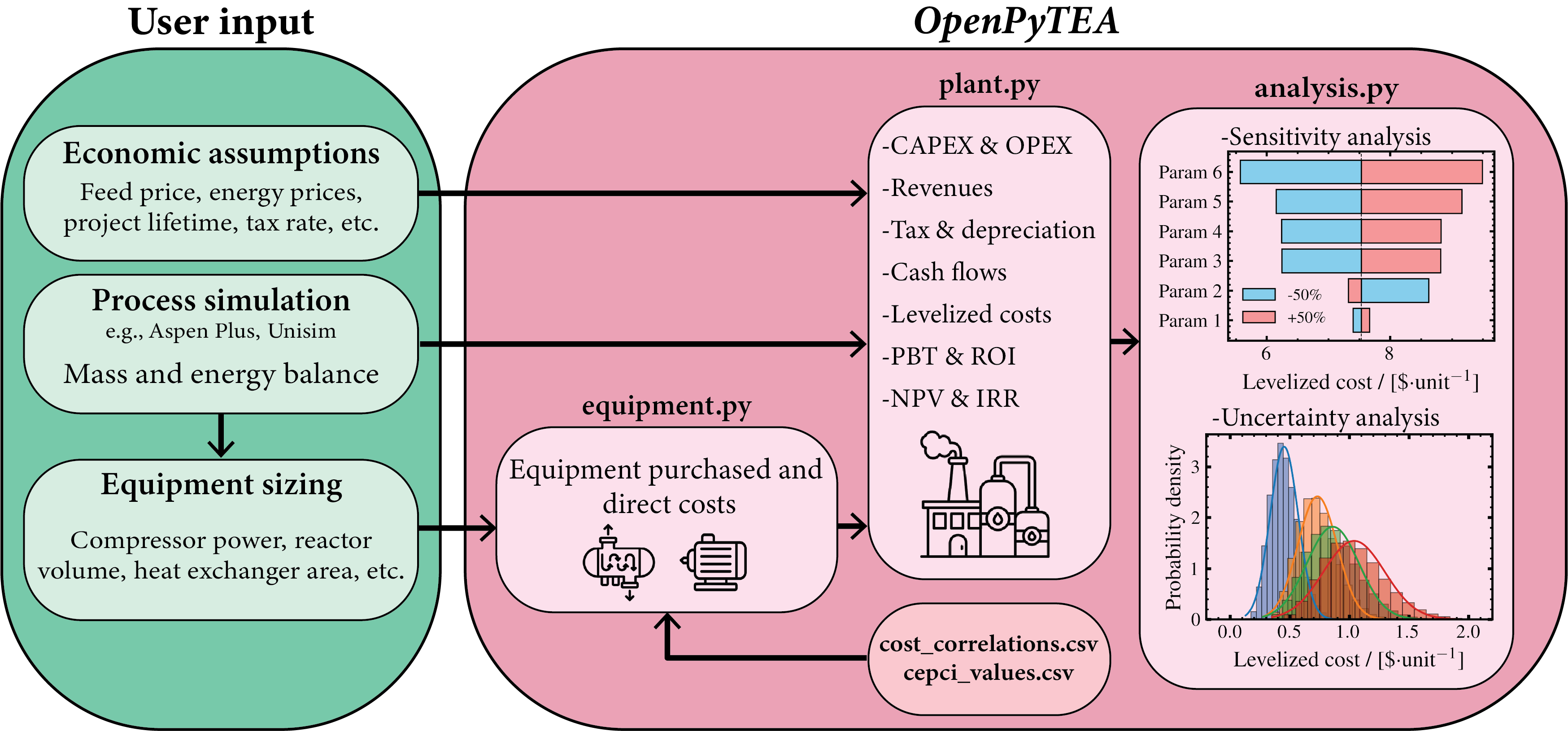
|
15
|
+
Requires-Dist: scipy>=1.10
|
|
16
|
+
Requires-Dist: tqdm>=4.64
|
|
17
|
+
Requires-Dist: jinja2>=3.1
|
|
18
|
+
Provides-Extra: test
|
|
19
|
+
Requires-Dist: pytest>=8.0; extra == "test"
|
|
20
|
+
Provides-Extra: ipython
|
|
21
|
+
Requires-Dist: ipython>=8.0; extra == "ipython"
|
|
22
|
+
Requires-Dist: ipywidgets>=8.0; extra == "ipython"
|
|
23
|
+
Dynamic: license-file
|
|
24
|
+
|
|
25
|
+
<p align="center">
|
|
26
|
+
<img src="https://raw.githubusercontent.com/pbtamarona/OpenPyTEA/main/docs/logo-white.png" alt="OpenPyTEA" width="400"/>
|
|
27
|
+
</p>
|
|
28
|
+
|
|
29
|
+
**OpenPyTEA** is an open-source Python toolkit for performing **techno-economic assessment (TEA)** of chemical and energy systems. It was created to address a persistent gap in the TEA workflow: while process simulators model mass and energy balances, researchers often lack an equally transparent and flexible way to evaluate the **economic feasibility** of their designs. Commercial tools remain *black-box tools*, and many academic TEA implementations are process-specific, undocumented, or difficult to reproduce.
|
|
30
|
+
|
|
31
|
+
**OpenPyTEA** provides a fully open, modular, and traceable framework that brings TEA into the Python ecosystem. By integrating **equipment cost estimation**, **capital and operating expenditure modeling**, **cash-flow analysis**, **cost breakdowns**, **sensitivity evaluation**, and **Monte Carlo uncertainty propagation**, the toolkit enables users to perform end-to-end TEA with clarity and reproducibility.
|
|
32
|
+
|
|
33
|
+
Beyond its functionality, **OpenPyTEA is designed as a community-driven TEA platform**. Users can contribute new equipment cost correlations, improve economic models, report issues, and expand the toolkit’s capabilities over time. This collaborative approach helps build a shared, transparent, and continually improving TEA resource—similar to the open-source progress seen in the LCA community.
|
|
34
|
+
|
|
35
|
+
Whether used for early-stage process design, technology screening, or teaching, **OpenPyTEA** makes TEA more accessible, consistent, and aligned with FAIR research principles (Findable, Accessible, Interoperable, and Reusable).
|
|
36
|
+
|
|
37
|
+
**For a full walkthrough of the features and usage of OpenPyTEA, refer to the `walkthrough.ipynb` notebook**:
|
|
38
|
+
https://github.com/pbtamarona/OpenPyTEA/blob/main/walkthrough.ipynb
|
|
39
|
+
|
|
40
|
+
**For the full documentation of the package, visit the ReadTheDocs page:**
|
|
41
|
+
https://openpytea.readthedocs.io
|
|
42
|
+
|
|
43
|
+
**For some case-study examples, please check the `examples` folder:**
|
|
44
|
+
https://github.com/pbtamarona/OpenPyTEA/tree/main/examples
|
|
45
|
+
|
|
46
|
+
---
|
|
47
|
+
## 🎓 Workshop
|
|
48
|
+
|
|
49
|
+
We are hosting a one-day workshop on open-science techno-economic assessment using **OpenPyTEA**!
|
|
50
|
+
|
|
51
|
+
<p align="center">
|
|
52
|
+
<img src="https://raw.githubusercontent.com/pbtamarona/OpenPyTEA/main/workshop-flyer.jpg" alt="OpenPyTEA" width="800"/>
|
|
53
|
+
</p>
|
|
54
|
+
|
|
55
|
+
**Open-Science Techno-Economic Assessment with OpenPyTEA: From Process Design to Economic Insights**
|
|
56
|
+
|
|
57
|
+
The workshop covers the full workflow from process design and simulation to economic evaluation, combining lectures, a hands-on session with OpenPyTEA, and an industry talk by Shell. It closes with a community discussion on establishing shared TEA standards, bringing together students, researchers, engineers, and policymakers across chemical, energy, and sustainability sciences.
|
|
58
|
+
|
|
59
|
+
- 📅 **Date:** November 6, 2026 | 09:30 – 18:00
|
|
60
|
+
- 📍 **Location:** Process & Energy, TU Delft, Delft, The Netherlands
|
|
61
|
+
- 📝 **Registration:** [aanmelder.nl/openpytea2026](https://aanmelder.nl/openpytea2026)
|
|
62
|
+
- ⏰ **Deadline:** $${\color{red}\textbf{Registration closes on October 15, 2026}}$$
|
|
63
|
+
|
|
64
|
+
Lunch, snacks, coffee, and drinks will be provided!
|
|
65
|
+
|
|
66
|
+
---
|
|
67
|
+
## ✨ Key Features
|
|
68
|
+
- **Modular architecture:** clean separation of cost correlations, equipment objects, plant economics, and uncertainty analysis.
|
|
69
|
+
- **Transparent and reproducible:** all algorithms, equations, and assumptions are openly available for full traceability.
|
|
70
|
+
- **Cost breakdown visualization:** built-in functions to plot stacked bar charts of equipment costs, fixed capital, operating costs, and levelized cost of production (LCOP).
|
|
71
|
+
- **Cash flow diagrams:** visualize a project's cumulative cash flow over time, including its maximum investment and pay-back point, with support for overlaying multiple plants.
|
|
72
|
+
- **Built-in uncertainty tools:** automatic generation of sensitivity plots and Monte Carlo simulations, covering process quantities (consumption and production rates) as well as prices and financial assumptions.
|
|
73
|
+
- **Parameter dependencies:** declare how quantities depend on one another — cooling water scaling with production, a byproduct's yield tracking the main product, capital cost scaling with capacity — and every analysis honours the same graph.
|
|
74
|
+
- **Workflow using JSON configuration files:** standardized input/output structure via `io.py` for reproducible analyses and multi-scenario evaluation.
|
|
75
|
+
- **Flexible analysis and visualization:** separation of data processing (`analysis.py`) and plotting (`plotting.py`) allows users to apply custom visualization tools.
|
|
76
|
+
- **Interoperable and extensible:** easy integration with process simulators, optimization frameworks, and LCA tools.
|
|
77
|
+
- **Education-friendly:** ideal for teaching TEA and process design without reliance on proprietary software.
|
|
78
|
+
- **Community-driven:** users can contribute new correlations, improve models, request features, and shape the evolution of the platform.
|
|
79
|
+
|
|
80
|
+
---
|
|
81
|
+
## 📦 Installation
|
|
82
|
+
|
|
83
|
+
### 1. **Install from PyPI (recommended)**
|
|
84
|
+
|
|
85
|
+
```bash
|
|
86
|
+
pip install openpytea
|
|
87
|
+
```
|
|
88
|
+
|
|
89
|
+
### 2. **Install from GitHub (development version)**
|
|
90
|
+
|
|
91
|
+
```bash
|
|
92
|
+
pip install git+https://github.com/pbtamarona/OpenPyTEA
|
|
93
|
+
```
|
|
94
|
+
|
|
95
|
+
or with `uv`:
|
|
96
|
+
|
|
97
|
+
```bash
|
|
98
|
+
uv add git+https://github.com/pbtamarona/OpenPyTEA
|
|
99
|
+
```
|
|
100
|
+
|
|
101
|
+
**OpenPyTEA** requires **Python ≥ 3.10**.
|
|
102
|
+
The main dependencies include:
|
|
103
|
+
|
|
104
|
+
- `matplotlib`
|
|
105
|
+
- `numpy`
|
|
106
|
+
- `pandas`
|
|
107
|
+
- `scienceplots`
|
|
108
|
+
- `scipy`
|
|
109
|
+
- `tqdm`
|
|
110
|
+
- `jinja2`
|
|
111
|
+
|
|
112
|
+
---
|
|
113
|
+
## ⚙️ Package (Repository) Structure
|
|
114
|
+
```
|
|
115
|
+
src/openpytea/
|
|
116
|
+
├── equipment.py # Equipment-level costing and inflation correction
|
|
117
|
+
├── plant.py # Plant-level TEA: CAPEX, OPEX, cash flows, financial metrics
|
|
118
|
+
├── analysis.py # Sensitivity and uncertainty analysis (sensitivity plots, Monte Carlo)
|
|
119
|
+
├── plotting.py # Visualization functions (plots and figures)
|
|
120
|
+
├── io.py # JSON-based workflow: load inputs and export results
|
|
121
|
+
├── helpers.py # Helper functions for data handling and common operations
|
|
122
|
+
└── data/ # Cost correlations database and CEPCI data
|
|
123
|
+
examples/ # Example notebooks and case studies
|
|
124
|
+
walkthrough.ipynb # Walkthrough of the package
|
|
125
|
+
pyproject.toml
|
|
126
|
+
README.md
|
|
127
|
+
```
|
|
128
|
+
|
|
129
|
+
---
|
|
130
|
+
## 🏗️ Software Architecture
|
|
131
|
+
|
|
132
|
+
|
|
133
|
+
|
|
134
|
+
Software architecture and data flow of **OpenPyTEA**, illustrating the progression from user input to TEA output. Users provide economic assumptions, process simulation results, and equipment-sizing parameters. Equipment-sizing information is linked with cost correlations and CEPCI values stored in CSV databases to calculate inflation-adjusted purchased and direct costs. `Equipment` objects are aggregated into a `Plant` object, where CAPEX, OPEX, and financial performance metrics are evaluated. The `analysis.py` module subsequently operates on `Plant` objects to perform sensitivity and uncertainty analyses.
|
|
135
|
+
|
|
136
|
+
---
|
|
137
|
+
## 🖥️ Graphical User Interface
|
|
138
|
+
|
|
139
|
+
> **Note:** The GUI is still in development and may not yet offer all the features of the Python package.
|
|
140
|
+
|
|
141
|
+
An optional graphical interface provides the full TEA workflow — equipment costing, plant configuration, results, sensitivity/tornado analysis, Monte Carlo, and multi-plant comparison — without writing Python code. It can be installed as a standalone desktop app — installers for **Windows** (`.exe`/`.msi`) and **macOS** (`.dmg`) are available on the [Releases page](https://github.com/pbtamarona/OpenPyTEA/releases), with no Python or Node.js required — or run from source as a FastAPI + React application.
|
|
142
|
+
|
|
143
|
+
The GUI's source, installer build, setup instructions, and architecture documentation live on the [`standalone-package`](https://github.com/pbtamarona/OpenPyTEA/tree/standalone-package) branch:
|
|
144
|
+
|
|
145
|
+
```bash
|
|
146
|
+
git fetch origin
|
|
147
|
+
git checkout standalone-package
|
|
148
|
+
```
|
|
149
|
+
|
|
150
|
+
---
|
|
151
|
+
## 🧠 Core Concepts
|
|
152
|
+
|
|
153
|
+
### 1. **Equipment-level costing**
|
|
154
|
+
|
|
155
|
+
Each process unit (e.g., compressor, heat exchanger, reactor) is represented by an `Equipment` object:
|
|
156
|
+
|
|
157
|
+
```python
|
|
158
|
+
from openpytea.equipment import Equipment
|
|
159
|
+
|
|
160
|
+
compressor = Equipment(
|
|
161
|
+
name='COMP',
|
|
162
|
+
param=5000, # kW
|
|
163
|
+
process_type='Fluids',
|
|
164
|
+
category='Compressors, fans, & Blowers',
|
|
165
|
+
type='Compressor, centrifugal',
|
|
166
|
+
material='Carbon steel'
|
|
167
|
+
)
|
|
168
|
+
|
|
169
|
+
print(compressor.direct_cost)
|
|
170
|
+
```
|
|
171
|
+
|
|
172
|
+
Each equipment item retrieves its cost correlation from the internal database in `data/cost_correlations.csv` and adjusts the cost to the desired year using the Chemical Engineering Plant Cost Index (CEPCI).
|
|
173
|
+
|
|
174
|
+
Assemblies such as a PSA skid (vessels plus adsorbent layers) can be built from individually priced sub-components with `CompositeEquipment`; the composite then behaves like any other equipment item in a plant:
|
|
175
|
+
|
|
176
|
+
```python
|
|
177
|
+
from openpytea.equipment import CompositeEquipment
|
|
178
|
+
|
|
179
|
+
psa = CompositeEquipment(
|
|
180
|
+
name='PSA',
|
|
181
|
+
process_type='Fluids',
|
|
182
|
+
components=[vessel, zeolite, carbon], # ordinary Equipment objects
|
|
183
|
+
)
|
|
184
|
+
print(psa.direct_cost)
|
|
185
|
+
psa.breakdown() # one row per sub-component
|
|
186
|
+
```
|
|
187
|
+
|
|
188
|
+
### 2. **Plant-level techno-economic assessment**
|
|
189
|
+
|
|
190
|
+
Multiple equipment objects can be grouped into a `Plant` instance for full TEA
|
|
191
|
+
|
|
192
|
+
```python
|
|
193
|
+
from openpytea.plant import Plant
|
|
194
|
+
|
|
195
|
+
ammonia_plant = Plant({
|
|
196
|
+
'plant_name': 'Ammonia Production Plant',
|
|
197
|
+
'country': 'Netherlands',
|
|
198
|
+
'process_type': 'Fluids',
|
|
199
|
+
'equipment': [compressor],
|
|
200
|
+
'interest_rate': 0.09,
|
|
201
|
+
'plant_utilization': 0.95,
|
|
202
|
+
'project_lifetime': 20, # in years
|
|
203
|
+
'plant_products': { # Here we define the product(s) of the plant
|
|
204
|
+
'ammonia': {
|
|
205
|
+
'production': 125_000, # Daily production in kg/day
|
|
206
|
+
}
|
|
207
|
+
},
|
|
208
|
+
'variable_opex_inputs': {
|
|
209
|
+
'electricity': {
|
|
210
|
+
'consumption': 110, # Daily consumption, in MWh
|
|
211
|
+
'price': 75 # US$/MWh
|
|
212
|
+
},
|
|
213
|
+
'hydrogen': {
|
|
214
|
+
'consumption': 22_000, # Daily consumption, in kg/day
|
|
215
|
+
'price': 2 # US$/kg
|
|
216
|
+
},
|
|
217
|
+
},
|
|
218
|
+
})
|
|
219
|
+
|
|
220
|
+
ammonia_plant.calculate_cash_flow(print_results=True)
|
|
221
|
+
ammonia_plant.calculate_levelized_cost()
|
|
222
|
+
```
|
|
223
|
+
Main outputs include:
|
|
224
|
+
- Capital expenditures (CAPEX): inside/outside battery limits, engineering, contingency, and location factors
|
|
225
|
+
- Operating expenditures (OPEX): variable and operating expenditures, including utilities, maintenance, labor, and overhead costs
|
|
226
|
+
- Financial metrics: Net Present Value (NPV), Internal Rate of Return (IRR), Return on Investment (ROI), Payback Time (PBT), and Levelized Cost of Product (LCOP)
|
|
227
|
+
|
|
228
|
+
### 3. **CAPEX and OPEX breakdown plots**
|
|
229
|
+
|
|
230
|
+
Following a `data` + `plot` pattern used throughout the package, OpenPyTEA includes convenience functions for visualizing the economic structure of one or more plants as stacked bar charts:
|
|
231
|
+
|
|
232
|
+
- `direct_costs_data()` + `plot_stacked_bar()`: direct equipment costs (per equipment item; `expand_composites=True` splits composite equipment into its components).
|
|
233
|
+
- `fixed_capital_data()` + `plot_stacked_bar()`: fixed capital components (ISBL, OSBL, design & engineering, contingency).
|
|
234
|
+
- `variable_opex_data()` + `plot_stacked_bar()`: variable operating costs by input mass and energy stream.
|
|
235
|
+
- `fixed_opex_data()` + `plot_stacked_bar()`: fixed operating expenses, including labor, supervision, maintenance, overhead, R&D, and more.
|
|
236
|
+
- `levelized_cost_data()` + `plot_stacked_bar()`: levelized cost of production (LCOP), broken down into discounted CAPEX, OPEX, and side-product revenue.
|
|
237
|
+
|
|
238
|
+
```python
|
|
239
|
+
from openpytea.analysis import direct_costs_data, levelized_cost_data
|
|
240
|
+
from openpytea.plotting import plot_stacked_bar
|
|
241
|
+
|
|
242
|
+
direct_costs = direct_costs_data(ammonia_plant)
|
|
243
|
+
fig, ax = plot_stacked_bar(direct_costs)
|
|
244
|
+
|
|
245
|
+
lcop = levelized_cost_data(ammonia_plant)
|
|
246
|
+
fig, ax = plot_stacked_bar(lcop)
|
|
247
|
+
```
|
|
248
|
+
|
|
249
|
+
Each `*_data()` function also accepts a **list of plants**, in which case `plot_stacked_bar` draws one bar per plant side-by-side for direct comparison. Separating data preparation (`analysis.py`) from plotting (`plotting.py`) means you can also feed the returned dictionaries into your own custom visualization code.
|
|
250
|
+
|
|
251
|
+
### 4. **Cash flow diagram**
|
|
252
|
+
|
|
253
|
+
`cash_flow_data()` and `plot_cash_flow()` visualize a project's cumulative cash flow over time: the dip into debt during construction, the point of maximum investment, the break-even (pay-back) point, and the eventual climb into profit.
|
|
254
|
+
|
|
255
|
+
```python
|
|
256
|
+
from openpytea.analysis import cash_flow_data
|
|
257
|
+
from openpytea.plotting import plot_cash_flow
|
|
258
|
+
|
|
259
|
+
cash_flow = cash_flow_data(ammonia_plant)
|
|
260
|
+
fig, ax = plot_cash_flow(cash_flow)
|
|
261
|
+
```
|
|
262
|
+
|
|
263
|
+
As with the cost breakdowns, passing a **list of plants** overlays their cumulative cash flow curves — each with its own shaded debt region and break-even line — for direct comparison. The returned dictionary also carries the underlying figures (`max_investment`, `max_investment_year`, `breakeven_year`/`payback_time`) for use outside the plot, e.g. in reports.
|
|
264
|
+
|
|
265
|
+
### 5. **Sensitivity and uncertainty analysis**
|
|
266
|
+
|
|
267
|
+
**OpenPyTEA** provides integrated tools for visual sensitivity and probabilistic analysis of cost and performance drivers.
|
|
268
|
+
|
|
269
|
+
One-Way Sensitivity Line Plot
|
|
270
|
+
```python
|
|
271
|
+
from openpytea.analysis import sensitivity_data
|
|
272
|
+
from openpytea.plotting import plot_sensitivity
|
|
273
|
+
|
|
274
|
+
results = sensitivity_data(
|
|
275
|
+
ammonia_plant,
|
|
276
|
+
parameter="electricity",
|
|
277
|
+
plus_minus_value=0.5,
|
|
278
|
+
)
|
|
279
|
+
fig, ax = plot_sensitivity(results)
|
|
280
|
+
```
|
|
281
|
+
The `plants` input may also be a list of `Plant` objects to generate comparison plots.
|
|
282
|
+
|
|
283
|
+
Besides prices and financial assumptions, `parameter` also accepts a **process quantity** — `"electricity.consumption"` or `"ammonia.production"` — to sweep the physical side of the plant.
|
|
284
|
+
|
|
285
|
+
Tornado Plot (One-at-a-Time Sensitivity)
|
|
286
|
+
```python
|
|
287
|
+
from openpytea.analysis import tornado_data
|
|
288
|
+
from openpytea.plotting import plot_tornado
|
|
289
|
+
|
|
290
|
+
results = tornado_data(ammonia_plant, plus_minus_value=0.5)
|
|
291
|
+
fig, ax = plot_tornado(results)
|
|
292
|
+
```
|
|
293
|
+
Pass `include_process_params=True` to rank consumption and production quantities alongside the prices and financial assumptions.
|
|
294
|
+
|
|
295
|
+
Monte Carlo Simulation
|
|
296
|
+
```python
|
|
297
|
+
from openpytea.analysis import monte_carlo
|
|
298
|
+
from openpytea.plotting import plot_monte_carlo
|
|
299
|
+
|
|
300
|
+
results = monte_carlo(ammonia_plant, num_samples=1_000_000)
|
|
301
|
+
fig, ax = plot_monte_carlo(results)
|
|
302
|
+
```
|
|
303
|
+
Outputs include probability distributions and confidence intervals for LCOP, NPV, ROI, and payback time—supporting uncertainty-informed decision-making. With `plot_multiple_monte_carlo`, **OpenPyTEA** can also visualize Monte Carlo results for multiple plants to enable uncertainty comparisons. `plot_monte_carlo_inputs` shows the sampled inputs themselves, split into **process** and **economic** figures, to confirm each distribution came out as intended.
|
|
304
|
+
|
|
305
|
+
Uncertainty is configured per item: `price_uncertainty` on any `variable_opex_inputs` or `plant_products` entry, `consumption_uncertainty`/`production_uncertainty` for the quantities, and `project_uncertainties` for the project-level scalars.
|
|
306
|
+
|
|
307
|
+
Parameter Dependencies
|
|
308
|
+
```python
|
|
309
|
+
ammonia_plant.update_configuration({
|
|
310
|
+
"variable_opex_inputs": {
|
|
311
|
+
"hydrogen": {
|
|
312
|
+
"consumption_dependency": {
|
|
313
|
+
"depends_on": {"production:ammonia": 0.176}, # kg H2 per kg NH3
|
|
314
|
+
},
|
|
315
|
+
},
|
|
316
|
+
},
|
|
317
|
+
})
|
|
318
|
+
```
|
|
319
|
+
Rather than varying independently, a quantity can be defined as a linear function of one or more others — `dependent = Σ wᵢ · parentᵢ + offset`. Here the hydrogen feed follows ammonia production instead of drifting away from it. Process and economic parameters can drive each other in either direction (a byproduct's yield tracking the main product, `fixed_capital_factor` scaling with capacity), chains and multi-parent nodes resolve automatically, and cycles raise an error. A dependent may carry its own additive `noise` on top of the implied mean.
|
|
320
|
+
|
|
321
|
+
Because dependencies live on the `Plant`, **all three analyses honour them**: Monte Carlo samples through the graph, while `sensitivity_data` and `tornado_data` propagate each perturbation through it and refuse to vary a parameter that a dependency already determines. See the Analysis user guide in the [documentation](https://openpytea.readthedocs.io) for the full configuration format.
|
|
322
|
+
|
|
323
|
+
### 6. **Workflow using JSON config files and command-line interface**
|
|
324
|
+
|
|
325
|
+
**OpenPyTEA** supports a workflow using structured JSON input files via the `io.py` module. This enables standardized, reproducible, and scalable TEA studies.
|
|
326
|
+
|
|
327
|
+
Key functionalities include:
|
|
328
|
+
- `run_equipment()`: evaluate equipment costs from JSON input
|
|
329
|
+
- `run_plant()`: construct and evaluate a plant configuration
|
|
330
|
+
- `run_tea()`: execute full TEA, including cost breakdowns, sensitivity, and uncertainty analysis
|
|
331
|
+
- `run_openpytea()`: single-file counterpart to `run_tea()` — runs the same pipeline from one combined JSON file (`equipment` + `plant` + `analysis` blocks), intended for CLI use
|
|
332
|
+
|
|
333
|
+
This workflow is demonstrated in `case_study_1_with_JSON.ipynb` in the example folder.
|
|
334
|
+
|
|
335
|
+
Installing **OpenPyTEA** also installs an `openpytea` command-line tool, so the same combined-file workflow can be run without writing any Python:
|
|
336
|
+
|
|
337
|
+
```bash
|
|
338
|
+
openpytea run project/config.json --output-dir outputs/tea_results
|
|
339
|
+
```
|
|
340
|
+
|
|
341
|
+
`openpytea equipment`, `openpytea plant`, and `openpytea tea` (the three-file variant of `run_tea()`) are also available — run `openpytea --help` for the full command list. See the [JSON Workflow guide](docs/user_guide/io_workflow.rst) for details.
|
|
342
|
+
|
|
343
|
+
---
|
|
344
|
+
## 📘 Example Workflows
|
|
345
|
+
|
|
346
|
+
Example notebooks are available in the `examples/` folder, including:
|
|
347
|
+
|
|
348
|
+
- Comparison of hydrogen production pathwways
|
|
349
|
+
- Hydrogen liquefaction precooling system
|
|
350
|
+
- Geothermal-based heating and power generation
|
|
351
|
+
|
|
352
|
+
Run any example via:
|
|
353
|
+
```bash
|
|
354
|
+
jupyter notebook examples/case_study_1.ipynb
|
|
355
|
+
```
|
|
356
|
+
Each notebook demonstrates:
|
|
357
|
+
- Input definition and equipment configuration
|
|
358
|
+
- Cash-flow and investment evaluation
|
|
359
|
+
- Sensitivity and uncertainty analysis
|
|
360
|
+
- Visualization of key economic indicators
|
|
361
|
+
|
|
362
|
+
---
|
|
363
|
+
## 🧑🏫 Educational Use
|
|
364
|
+
|
|
365
|
+
**OpenPyTEA** is suitable for chemical and process engineering education.
|
|
366
|
+
Students can perform full TEA using their simulation outputs—estimating capital, operating, and profitability metrics—without commercial software.
|
|
367
|
+
All algorithms are visible and modifiable, eliminating the “black-box” nature of most TEA tools.
|
|
368
|
+
|
|
369
|
+
---
|
|
370
|
+
## 🛠️ Contributing
|
|
371
|
+
We welcome community contributions!
|
|
372
|
+
You can help by:
|
|
373
|
+
- Adding or updating equipment cost correlations
|
|
374
|
+
- Improving the documentation or creating tutorials
|
|
375
|
+
- Extending the visualization or uncertainty modules
|
|
376
|
+
|
|
377
|
+
To contribute:
|
|
378
|
+
1. Fork the repository.
|
|
379
|
+
2. Create a new branch:
|
|
380
|
+
```bash
|
|
381
|
+
git checkout -b feature-new-equipment
|
|
382
|
+
```
|
|
383
|
+
3. Commit your changes and open a Pull Request.
|
|
384
|
+
|
|
385
|
+
Please follow PEP8 coding conventions and include a short description of your updates.
|
|
386
|
+
|
|
387
|
+
---
|
|
388
|
+
## 📖 Publication
|
|
389
|
+
|
|
390
|
+
**OpenPyTEA** is described in the following peer-reviewed paper published in *SoftwareX*:
|
|
391
|
+
|
|
392
|
+
> Tamarona, P.B., Vlugt, T.J.H., & Ramdin, M. (2026). *OpenPyTEA: An open-source python toolkit
|
|
393
|
+
> for techno-economic assessment of chemical process plants and energy systems with economic
|
|
394
|
+
> sensitivity and uncertainty evaluation.* SoftwareX, 35, 102816.
|
|
395
|
+
> https://doi.org/10.1016/j.softx.2026.102816
|
|
396
|
+
|
|
397
|
+
If you use **OpenPyTEA** in your research, please cite this paper (see [Citation](#-citation) below).
|
|
398
|
+
|
|
399
|
+
---
|
|
400
|
+
## 📚 Citation
|
|
401
|
+
|
|
402
|
+
If you use **OpenPyTEA** in your research, please cite the following paper:
|
|
403
|
+
|
|
404
|
+
> Tamarona, P.B., Vlugt, T.J.H., & Ramdin, M. (2026). *OpenPyTEA: An open-source python toolkit
|
|
405
|
+
> for techno-economic assessment of chemical process plants and energy systems with economic
|
|
406
|
+
> sensitivity and uncertainty evaluation.* SoftwareX, 35, 102816.
|
|
407
|
+
> https://doi.org/10.1016/j.softx.2026.102816
|
|
408
|
+
|
|
409
|
+
**BibTeX:**
|
|
410
|
+
```bibtex
|
|
411
|
+
@article{TAMARONA2026102816,
|
|
412
|
+
title = {OpenPyTEA: An open-source python toolkit for techno-economic assessment of chemical process plants and energy systems with economic sensitivity and uncertainty evaluation},
|
|
413
|
+
journal = {SoftwareX},
|
|
414
|
+
volume = {35},
|
|
415
|
+
pages = {102816},
|
|
416
|
+
year = {2026},
|
|
417
|
+
issn = {2352-7110},
|
|
418
|
+
doi = {https://doi.org/10.1016/j.softx.2026.102816},
|
|
419
|
+
url = {https://www.sciencedirect.com/science/article/pii/S2352711026003080},
|
|
420
|
+
author = {P.B. Tamarona and T.J.H. Vlugt and M. Ramdin},
|
|
421
|
+
keywords = {Techno-economic assessment, Process design, Process plant, Power plant, Chemical engineering},
|
|
422
|
+
` ` `
|
|
423
|
+
```
|
|
424
|
+
|
|
425
|
+
---
|
|
426
|
+
## 📄 License
|
|
427
|
+
|
|
428
|
+
**OpenPyTEA** is released under the MIT License.
|
|
429
|
+
|
|
430
|
+
You are free to use, modify, and distribute the code with proper attribution.
|
|
431
|
+
|
|
432
|
+
---
|
|
433
|
+
## 📬 Contact
|
|
434
|
+
Panji B. Tamarona
|
|
435
|
+
|
|
436
|
+
📧 P.B.Tamarona@tudelft.nl
|
|
437
|
+
|
|
438
|
+
Repository: https://github.com/pbtamarona/OpenPyTEA
|